Synchronization in asymmetrically coupled networks with node balance

CHAOS 16, 015102 共2006兲

Synchronization in asymmetrically coupled networks with node balance Igor Belykha兲 Department of Mathematics and Statistics, Georgia State University, Atlanta, Georgia 30303 and School of Computer and Communication Sciences, Ecole Polytechnique Fédérale de Lausanne (EPFL), Station 14, 1015 Lausanne, Switzerland

Vladimir Belykh Department of Mathematics, Volga State Academy, 5, Nesterov st., Nizhny Novgorod 603 600, Russia

Martin Hasler School of Computer and Communication Sciences, Ecole Polytechnique Fédérale de Lausanne (EPFL), Station 14, 1015 Lausanne, Switzerland

共Received 22 September 2005; accepted 9 November 2005; published online 31 March 2006兲 We study global stability of synchronization in asymmetrically connected networks of limit-cycle or chaotic oscillators. We extend the connection graph stability method to directed graphs with node balance, the property that all nodes in the network have equal input and output weight sums. We obtain the same upper bound for synchronization in asymmetrically connected networks as in the network with a symmetrized matrix, provided that the condition of node balance is satisfied. In terms of graphs, the symmetrization operation amounts to replacing each directed edge by an undirected edge of half the coupling strength. It should be stressed that without node balance this property in general does not hold. © 2006 American Institute of Physics. 关DOI: 10.1063/1.2146180兴 The simplest and most striking interaction between dynamical systems is their synchronization. Individual dynamical systems with trajectories that are quite different can be brought to follow exactly or approximately the same trajectory, through interaction in a network. Stable synchrony can be achieved in many different types of asymmetrically or symmetrically connected oscillator networks as long as the coupling between the nodes is strong enough. The symmetry of coupling essentially facilitates the analytical study and allows the derivation of synchronization conditions from graph theoretical quantities using the connection graph method. In this paper we show that the symmetry of undirected graphs can also be used for the study of synchronization in asymmetrically connected networks with node balance. Node balance means that the sum of the coupling coefficients of all edges directed to a node equals the sum of the coupling coefficients of all edges directed outward from the node. This property allows us to derive an elegant graph-based criterion for synchronization in directed networks. We prove that for node balanced networks it is sufficient to symmetrize all connections by replacing a unidirectional coupling with a bidirectional coupling of half the coupling strength. The synchronization condition for the symmetrized network then also guarantees synchronization in the original asymmetrical network.

I. INTRODUCTION

Networks of dynamical systems have been used in physics and biology for decades, and they are now becoming a兲

Electronic mail: [email protected]

1054-1500/2006/16共1兲/015102/9/$23.00

more and more relevant for engineering and computer sciences.1 The purpose to connect dynamical systems in networks is to get them to solve problems cooperatively. In physics, this is the origin of cooperative phenomena such as, e.g., phase transitions. In biology, complex networks of chemical reactions take place in all living organisms. In particular, such networks are used for information processing in the brain.2 The simplest mode of the coordinated motion between dynamical systems is their complete synchronization when all cells of the network acquire identical dynamical behavior. Such cooperative behavior of a network models neurons that synchronize,3 coupled synchronized lasers4 and networks of computer clocks,5 as well as many other selforganizing systems. Synchronization in networks of dynamical systems depends both on the stability of the individual systems dynamics and on the topology and the kind of their interaction.6–27 Typically, networks of limit-cycle oscillators are easy to synchronize6–8 whereas coupled chaotic oscillators9–11 are more resistant to synchronization. Synchronization properties of pulse-coupled and linearly coupled networks can also be dramatically different.12 The influence of network topology on the stability of a synchronized motion where the motion could be a limit cycle or a chaotic attractor is currently a hot research topic. The conditions for complete synchronization of linearly coupled identical dynamical systems are composed of a term that depends only on the individual systems and a term that depends only on the network structure.14–27 A general approach to the local stability of periodic or chaotic synchronization for any linear coupling scheme, called the master stability function, was developed by Pecora and Carroll.19

16, 015102-1

© 2006 American Institute of Physics

Downloaded 03 Apr 2006 to 131.96.241.65. Redistribution subject to AIP license or copyright, see http://chaos.aip.org/chaos/copyright.jsp

015102-2

Chaos 16, 015102 共2006兲

Belykh, Belykh, and Hasler

Within the framework of this powerful method, one proves local stability of the synchronization manifold by calculating analytically 共or numerically兲 the eigenvalues of the connectivity matrix and numerically the transversal Lyapunov exponents. This approach is widely used in studies of synchronization in complex networks with symmetrical28–30 or asymmetrical connections.31,32 Global stability results based on the calculation of the connectivity matrix eigenvalues were also derived for oscillator networks coupled via undirected33,34 and directed graphs.35 However, these eigenvalue based methods may be difficult to apply analytically for irregular graphs, especially defined by an asymmetrical connectivity matrix with complex eigenvalues, and these approaches in general fail for timedependent coupling coefficients.25,26 We have previously developed an alternative approach 共the connection graph method兲 to deriving rigorous bounds on the minimum coupling strength that is necessary to achieve complete synchronization from any initial, nonsynchronized state. The proof is based on Lyapunov functions and assumes symmetrical coupling 共undirected graphs兲. The term that depends on the network structure is derived from purely graph theoretic quantities. It allows us to derive individually the strength of coupling for any two symmetrically interacting systems such that the resulting network exhibits globally stable complete synchronization. The method directly links synchronization with graph theory and allows us to avoid calculating the eigenvalues of the connectivity matrix. It is also applicable to time-dependent networks. In this work we extend our approach to asymmetrically coupled networks. The connection graph of such a network is directed and the coupling coefficient from node i to node j is in general different from the coupling coefficient for the reverse direction. It turns out that we obtain the same criterion as for the network with a symmetrized connection matrix, provided that the condition of node balance is satisfied. Node balance means that the sum of the coupling coefficients of all edges directed to a node equals the sum of the coupling coefficients of all edges directed outward from the node. In the special case where all coupling coefficients are equal, this means that the in-degree equals the out-degree for each node, i.e., the number of edges coming into a vertex equals the number of edges going out of the vertex. In terms of graphs, the symmetrization operation amounts to replacing the edge directed from node i to node j by an undirected edge of half the coupling coefficient. In the case where there is an edge directed from node i to node j and another edge in the reverse direction, the pair of directed edges is replaced by an undirected edge with mean coupling coefficient. It should be stressed that without node balance the property in general does not hold. In particular, it is possible that an asymmetrically coupled network without node balance can never be synchronized, whereas the symmetrized network has a finite synchronization threshold.

n

x˙i = F共xi兲 + 兺 cik共t兲Pxk,

i = 1, . . . ,n.

共1兲

k=1

Here, xi = 共x1i , . . . , xdi 兲 is the d-vector containing the coordinates of the ith oscillator, and F共xi兲 is a nonlinear vector function defining the dynamics of the individual oscillator. The connectivity matrix C with entries cik is an n ⫻ n matrix with zero row-sums and non-negative off-diagonal elements n n cik = 0 and cii = −兺k=1;k⫽i cik, i = 1 , . . . , n. Matrix such that 兺k=1 C is assumed to be asymmetric, therefore it defines a directed 共nonreciprocal兲 graph C with n vertices and m edges. The vertices of the graph correspond to the individual oscillators, and the graph has an edge between node i and node j if at least one of the two coupling coefficients cij and c ji is nonzero. To allow complete synchronization of all the oscillators, the graph is assumed to be connected. Elements of the d ⫻ d matrix P determine which variables couple the oscillators. For clarity, we shall consider a vector version of the coupling with the diagonal matrix P = diag共p1 , p2 , . . . , pd兲, where ph = 1, h = 1 , 2 , . . . , s and ph = 0 for h = s + 1 , . . . , d. The generalization of all the results obtained in this paper for other possible cases of scalar and vector couplings between the oscillators is straightforward. We admit an arbitrary time dependence in the coupling matrix even if t is not explicitly stated everywhere. All constraints and criteria for the coupling matrix are understood to hold for all times t. The completely synchronous state of system 共1兲 is defined by the linear invariant manifold D = 兵x1 = x2 = ¯ = xn其, often called the synchronization manifold. In contrast to mutually coupled networks, where any connection graph configuration allows synchronization of all the nodes, synchrony in asymmetrically coupled networks is only possible if there is at least one node which directly or indirectly influences all the others. In terms of the connection graph, this amounts to the existence of a uniformly directed tree involving all the vertices. A star-coupled network where secondary nodes drive the hub is a counter example, where such a tree does not exist and synchronization is impossible. It is worth noticing that the connections of node i with the other nodes of the graph are defined by ith row and ith column elements of the matrix C. Connectivity matrices with both zero row and column sums correspond to node balanced networks, satisfying the property that all nodes in the network have equal input and output weight sums. We will use this property for deriving the synchronization criterion in Sec. III. We can give an interpretation of the node balance condition in terms of electrical currents. If we interpret each coupling coefficient as a current, flowing in the direction of the corresponding edge in the graph, then the node balance condition is nothing else than Kirchoff’s current laws. III. NETWORK SYNCHRONIZATION: A STABILITY CRITERION

II. NETWORK CONSIDERED

A. Decomposition of the connectivity matrix

We consider a network of n linearly coupled identical oscillators. The equations of motion read

Statement 1: Asymmetric connectivity matrix C = 兵cik其 can be decomposed into two n ⫻ n matrices E and ⌬:

Downloaded 03 Apr 2006 to 131.96.241.65. Redistribution subject to AIP license or copyright, see http://chaos.aip.org/chaos/copyright.jsp

015102-3

Chaos 16, 015102 共2006兲

Synchrony in node balanced networks

C = E + ⌬,

共2兲

where matrix E is symmetric

E = 兵␧ik其:

冦

␧ik = ␧ki = 21 共cik + cki兲 ␧ii = −

兺 共cik + cki兲 k=1;k⫽i

for k ⫽ i

⌬ = 兵␦ik其:

for k = i

冧

n

共3兲

k=1 n

+ 兺 兵␦ jk PX jk − ␦ik PXik其.

冦

␦ii = −

兺 共cik − cki兲, k=1;k⫽i

for k ⫽ i for k = i.

冧

共4兲

Taking into account only off-diagonal elements, the matrices E and ⌬ may be thought of as the symmetrized and antisymmetrized connectivity matrix C, respectively. Both n ␧ik = 0 and the matrices E and ⌬ have zero row sums: 兺k=1 n 兺k=1␦ik = 0, respectively. Statement 2: The diagonal elements of matrix ⌬ are ␦ii 1 n = 2 兺k=1cki. In other words, ␦ii is half the sum of ith column elements of the connectivity matrix C. The proof is straightforward. Adding and subtracting the n term 21 cii from ␦ii = − 21 兺k=1;k⫽i 共cik − cki兲, we obtain ␦ii 1 n 1 n = − 2 兺k=1cik + 2 兺k=1cki. The first term equals zero due to zero n row sums of the matrix C, therefore ␦ii = 21 兺k=1 cki. B. Application of the connection graph method

n

k=1

k=1

x˙i = F共xi兲 + 兺 ␧ik Pxk + 兺 ␦ik Pxk,

i = 1, . . . ,n.

共5兲

Introducing the notation for the differences Xij = x j − xi,

共6兲

i, j = 1, . . . ,n,

The origin O = 兵Xij = 0 , i , j = 1 , . . . , n其 is an equilibrium of the system 共8兲. Its global stability amounts to the global stability of the synchronization manifold D. Often, global stability of the equilibrium point O can be achieved through the coupling as long as it is strong enough to overcome the unstable term 关兰10DF共␤x j + 共1 − ␤兲xi兲d␤兴Xij, defining the divergence of coupled systems trajectories. The proof that the origin can be globally stable involves the construction of a Lyapunov function, a smooth, positive definite function that decreases along trajectories of the system 共8兲. To construct the Lyapunov function and obtain the conditions on the coupling strength required for global stability of synchronization in the network 共1兲, we shall follow the steps of our previous study of mutually connected networks.25 Adding and subtracting an additional term aPXij from the system 共8兲, we obtain X˙ij =

Our objective is to find a class of asymmetrically connected networks for which the connection graph 共stability兲 method can be directly applied. Using the decomposition 共2兲, we can rewrite Eq. 共1兲 in the form n

共8兲

k=1

n

1 2

DF共␤x j + 共1 − ␤兲xi兲d␤ Xij

+ 兺 兵␧ jk PX jk − ␧ik PXik其

and matrix ⌬ is antisymmetric

␦ik = 21 共cik − cki兲 = − ␦ki ,

册

1

0

n

1 2

冋冕

X˙ij =

25

similar to our previous work, we obtain the stability system for the difference variables

冋冕

X˙ij = F共x j兲 − F共xi兲 + 兺 兵␧ jk PX jk − ␧ik PXik其

DF共␤x j + 共1 − ␤兲xi兲d␤ − aP Xij + aPXij

0

n

n

k=1

k=1

+ 兺 兵␧ jk PX jk − ␧ik PXik其 + 兺 兵␦ jk PX jk − ␦ik PXik其,

冋冕

册

1

DF共␤x j + 共1 − ␤兲xi兲d␤ − aP Xij,

0

k=1

共10兲

i, j = 1, . . . ,n.

n

+ 兺 兵␦ jk PX jk − ␦ik PXik其.

共7兲

k=1

共9兲

where a is an auxiliary scalar parameter. The use of the auxiliary terms ±aPXij allows us to derive the stability conditions in two steps. The negative term −aPXij is favorable for the stability and added to damp instabilities caused by eigenvalues with positive real parts of the Jacobian DF. In turn, the corresponding positive term +aPXij can be damped by the coupling terms. Step 1: Introduce the auxiliary system X˙ij =

n

册

1

This system is the system 共9兲 without the coupling terms. Consider Lyapunov functions of the form

Using a compact vector notation for the function difference

冕 冋冕 1

F共x j兲 − F共xi兲 =

0

=

d F共␤x j + 共1 − ␤兲xi兲d␤ d␤ 1

0

Wij = 21 XTij · H · Xij,

册

DF共␤x j + 共1 − ␤兲xi兲d␤ Xij ,

where DF is a d ⫻ d Jacobi matrix of F, we obtain

i, j = 1, . . . ,n,

共11兲

where H = diag共h1 , h2 , . . . , hs , H1兲, h1 ⬎ 0 , . . . , hs ⬎ 0, and the 共d − s兲 ⫻ 共d − s兲 matrix H1 is positive definite. Assumption 1: The derivatives of the Lyapunov functions 共9兲 with respect to the system 共10兲 are required to be negative

Downloaded 03 Apr 2006 to 131.96.241.65. Redistribution subject to AIP license or copyright, see http://chaos.aip.org/chaos/copyright.jsp

015102-4

Chaos 16, 015102 共2006兲

Belykh, Belykh, and Hasler

˙ = XT H W ij ij

冋冕

册

1

DF共␤x j + 共1 − ␤兲xi兲d␤ − aP Xij ⬍ 0,

0

Xij ⫽ 0.

共12兲

In other words, we assume that there exists a critical value a*, sufficient to make the equilibrium state O of the auxiliary system 共10兲 globally stable. This is, in particular, the case if for arbitrary x the quadratic form XTijH共DF共x兲 − aP兲Xij is negative definite. Note that if a = c12, where c12 is the coupling strength in the network 共1兲 of two unidirectionally coupled oscillators 共the direction of coupling is unimportant兲, then the system 共10兲 becomes the stability system for synchronization in this simplest unidirectionally coupled network. Consequently, the assumption 共12兲 implies that the network 共1兲 of two unidirectionally coupled oscillators will be globally synchronized * . if the coupling exceeds the critical value c12 This is true for many coupled limit-cycle or chaotic systems. However, there are a few examples of coupled systems where increasing in coupling desynchronizes the network.15,20,21 Therefore, before proceeding with the study of synchronization in a larger network, we have to prove that the assumption 共12兲 holds for the chosen type of oscillators. Examples for which the proof is straightforward include coupled double-scrolls,14 Hindmarsh-Rose neuron models,27 Lorenz systems,25,36 etc. For example, for two unidirectionally x-coupled Lorenz oscillators: x˙1 = ␴共y 1 − x1兲 + c12共x2 − x1兲,

negative definite and favorable for the stability. Therefore, it has to be made large to overcome the contribution of the term S2. The last coupling term defined by the antisymmetric matrix ⌬ = 兵␦ij其 can change sign. In the following, we will show that this term equals zero for asymmetrically coupled networks with node balance, and therefore the symmetrical matrix E can give synchronization conditions for directed graphs defined by the asymmetric connectivity matrix C. Let us elaborate it. Using the symmetry of ␧, we can rewrite the third term S3 in the form25 n

n

S3 = − 兺 兺 兺

n−1 n

␧ jkXTjiHPX jk

i=1 j=1 k=1

Consider the fourth term n

n

S4 = −

1 2

n

兵␦ jkXTjiHPX jk + ␦ikXTikHPXij其. 兺 兺 兺 i=1 j=1 k=1

Renaming in the second term of S4 the summation index i by j and vice versa, this second term becomes identical to the first, and we get n

n

n

S4 = − 兺 兺 兺 ␦ jkXTjiHPX jk .

n

n

V=

兺 兺 i=1 j=1

n

XTij

· H · Xij ⬅

1 2

共13兲

n

兺 Wij . 兺 i=1 j=1

共14兲

n

n

n

n

1 2

兺 兺 W˙ij + i=1 j=1 n

−

1 2

1 2

n

共19兲

n

n

S共1兲 4

=−兺兺

n

XTjiHPX ji

i=1 j=1

␦ik = 0, 兺 k=1

共20兲

due to the zero row sums property of the matrix ⌬. Decompose the second term in Eq. 共19兲 n

=兺兺

n

␦ jjXTijHPXij

−兺 i=1

n

再

n

n

兺 ␦ jkXTjiHPXik 兺 j=1 k⫽j

冎

. 共21兲

For each i = 1 , . . . , n the sum in the second term of S共2兲 4 equals zero,

n

n

兺 兺 兵␦ jkXTjiHPX jk + ␦ikXTikHPXij其. 兺 i=1 j=1 k=1

− 兺 兺 兺 ␦ jkXTjiHPXik i=1 j=1 k=1

i=1 j=1

XTijaPXij 兺 兺 i=1 j=1

n

The first sum in Eq. 共19兲,

n

兺 兺 兵␧ jkXTjiHPX jk + ␧ikXTikHPXij其 兺 i=1 j=1 k=1 n

−

n

n

1 2

n

n

␦ jkXTjiHPX ji

共2兲 ⬅ S共1兲 4 + S4 .

S共2兲 4

The corresponding time derivative has the form V˙ =

共18兲

i=1 j=1 k=1

S4 = − 兺 兺 兺

y˙ 2 = rx2 − y 2 − x2z2 ,

assumption 共8兲 is true, and the bound for the synchronization coupling threshold is calculated as follows25 c* = 关b共b + 1兲共r + ␴兲2兴 / 关16共b − 1兲兴 − ␴. Step 2: Construct the Lyapunov function for the entire stability system 共9兲 1 4

共17兲

Using X jk = X ji + Xik, we decompose S4 into two sums

x˙2 = ␴共y 2 − x2兲,

z˙2 = − bz2 + x2y 2 ,

兺 n␧ jkXTjkHPX jk .

k=1 j⬎k

i=1 j=1 k=1

z˙1 = − bz1 + x1y 1,

=−兺

共16兲

n

y˙ 1 = rx1 − y 1 − x1z1,

n

共15兲

n ˙ is negative definite due to 兺nj=1W The first sum S1 = 21 兺i=1 ij n assumption 共8兲. The second sum S2 = 21 兺i=1 兺nj=1XTijaPXij is always positive definite. For convenience, it can be rewritten n−1 n 兺 j⬎iaXTij PXij, due to the symmetry as follows S2 = 兺i=1 2 2 2 共Xii = 0, Xij = X ji兲. As shown in the following, the third term S3 associated with the symmetrized matrix E = 兵␧ij其 is always

再

n

n

␦ jkXTjiHPXik 兺 兺 j=1 k⫽j

冎

= 0,

共22兲

due to the anti-symmetry of the matrix ⌬ : 兵␦ jk = −␦kj其 and the T equality XTjiHPXik = Xki HPXij. Consequently, we obtain n

n

T S共2兲 4 = 兺 兺 ␦ jjXij HPXij .

共23兲

i=1 j=1

Using the symmetry of the quadratic form S共2兲 4 , we get

Downloaded 03 Apr 2006 to 131.96.241.65. Redistribution subject to AIP license or copyright, see http://chaos.aip.org/chaos/copyright.jsp

015102-5

Chaos 16, 015102 共2006兲

Synchrony in node balanced networks n−1 n

S共2兲 4

= 兺 兺 ␮ijXTijHPXij ,

共24兲

i=1 j⬎i

where ␮ij = ␦ii + ␦ jj is half the sum of ith and jth column elements of the connectivity matrix C. Thus collecting the sums S2, S3, and S共2兲 4 from Eqs. 共15兲, 共16兲, and 共24兲, we obtain the condition that the time derivative V˙ is negative if n−1 n

兺 兺 XTijH关A − n␧ijP + ␮ijP兴Xij ⬍ 0. i=1 j⬎i

共25兲

The inequality 共25兲 is a sufficient condition for the global stability of the synchronization manifold. Due to zero row sums of the connectivity matrix C, the matrix 兵␮ij其 satisfies the condition n

兺 ␮ij = 0.

i,j=1

Then from the symmetry of the matrix 兵␮ij其, it follows n−1 n

兺 兺 ␮ij = 0. i=1 j⬎i

Thus, the coefficients ␮ij either equal zero or change sign along the set 兵1 艋 i 艋 n − 1 , i ⬍ j 艋 n其. Let us consider these two cases, separately. General case: ␮ij ⫽ 0. While negative ␮ij are favorable for the synchronization condition 共25兲, the contribution of positive ␮ij has to be compensated by the negative coupling terms. Therefore, the stability condition 共25兲 becomes dependent on the distribution of positive and negative coefficients ␮ij over all possible Xij , 兵1 艋 i 艋 n − 1 , i ⬍ j 艋 n其. The derivation of graph-based synchronization conditions for this general case requires consideration of an extended graph with additional edges corresponding to positive ␮ij. This will be reported elsewhere. The following is devoted to synchronization in networks for which ␮ij ⬅ 0. C. Synchrony in node balanced networks

It is easy to check that the constraint ␮ij ⬅ 0 relates to graphs with node balance. Hence, for such networks, the stability condition 共25兲 becomes n−1 n

兺 兺 XTijH关A − n␧ijP兴Xij ⬍ 0. i=1 j⬎i

共26兲

Here, the negative coupling term, defined by the symmetrical matrix E = 兵␧ij其, must overcome the contribution of the positive term XTijHAXij. The stability criterion 共26兲 for asymmetrically but node balanced networks is identical to the stability condition for symmetrized networks with the connectivity matrix E. Therefore, the connection graph method25 can be directly applied to this class of directed graphs. This results in the main statement of this paper. Theorem 1 (sufficient conditions): Under Assumption 1 and the assumption that the asymmetrical connectivity ma-

trix C = 兵cij其 has zero column sums (condition of node balance, ␮ij = 0兲, complete synchronization in the network (1) is globally asymptotically stable if cij共t兲 + c ji共t兲 a ⬅ ␧ij共t兲 ⬅ ␧k共t兲 ⬎ bk共n,m兲 2 n for k = 1, . . . ,m

and for all t,

共27兲

where at least one coefficient from the pair 共cij , c ji兲 is not zero and defines an edge on the directed connection graph C; the mean coupling coefficient ␧ij ⬅ ␧k defines edge k on the undirected graph E associated with the symmetrized matrix E; and bk共n , m兲 = 兺nj⬎i;k苸P 兩共Pij兲兩 is the sum of the lengths ij of all chosen paths Pij which pass through a given edge k that belongs to the undirected graph E. Here, m is the number of edges of the undirected graph rather than the original directed graph. In other words, we obtain the same criterion for synchronization in asymmetrically connected networks as for the network with a symmetrized connectivity matrix, provided that the condition of node balance is satisfied. In term of graphs, the symmetrization operation amounts to replacing the edge directed from node i to node j by an undirected edge of half the coupling coefficient. In the case where there is an edge directed from node i to node j and another edge in the reverse direction, the pair of directed edges is replaced by an undirected edge with mean coupling coefficient. Finally, the calculation of bk along the symmetrized undirected graph E gives us the stability condition for the asymmetrical network 共1兲. This calculation is straightforward within the framework of the connection graph method. To do so, we first choose a set of paths 兵Pij兩i , j = 1 , . . . , n , j典i其 共typically, the shortest paths兲, one for each pair of vertices i , j, and determine their lengths 兩Pij兩, the number of edges in each Pij. Then, for each edge k of the connection graph we calculate the sum bk共n , m兲 of the lengths of all Pij passing through k. Our previous works25,27 give further details on a possible choice of paths and calculations of bk共n , m兲 for different coupling configurations. Remark 1: Theorem 1 is not valid for unbalanced networks in general 关additional terms defined by the antisymmetric matrix ⌬ are always present in the stability condition 共25兲兴. Therefore, the symmetrization operation on the graph cannot be applied in general to directed unbalanced networks. Remark 2: Obviously, symmetrically coupled networks are always node balanced: zero row sums property of the symmetrical connectivity matrix C implies zero column sums. Therefore, Theorem 1 is applicable for such networks. However, the symmetrized matrix E will always be identical to C. For illustrative purposes, we can consider the simplest network of two symmetrically connected nodes with mutual coupling strength c. This network can also be considered as a ring of two unidirectionally connected oscillators. In terms of graphs, the symmetrization operation applied to both unidirectional links separately leaves us with two mutual halves of the coupling strength connections. Considered together, they form the original mutual coupling with strength c.

Downloaded 03 Apr 2006 to 131.96.241.65. Redistribution subject to AIP license or copyright, see http://chaos.aip.org/chaos/copyright.jsp

015102-6

Chaos 16, 015102 共2006兲

Belykh, Belykh, and Hasler asym ␭10 = − 2,

sym ␭10 = − 2.

Since the real parts of the eigenvalue of both networks are identical, by the master stability function approach19 it follows that both networks have the same local synchronization properties. It shows that our graph theoretical analysis correctly predicts the real relation between the two synchronization thresholds. B. Rings of K-nearest neighbor coupled oscillators

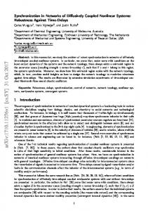
Quite similar results are obtained when analyzing the unidirectionally K-nearest neighbor coupled ring of dynamical systems 关see Fig. 1共b兲 共left兲 for K = 2兴 and its associated symmetrically coupled network of Fig. 1共b兲 共right兲. Our connection graph stability analysis of the latter yields the following sufficient condition for global synchronization:25 FIG. 1. Unidirectionally coupled networks and their symmetrized analogs with half the coupling strength per link. Arrows indicate direction of coupling along an edge; edges without arrows are coupled bidirectionally. The width of the links may be thought of as the coupling strength. 共a兲 Rings of locally coupled oscillators. 共b兲 Rings of K-nearest neighbor coupled oscillators. Here, K = 2 and n = 10.

IV. EXAMPLES A. Ring of unidirectionally coupled oscillators

Consider the unidirectionally coupled ring of dynamical systems, with constant coupling coefficient c 关Fig. 1共a兲 共left兲兴. At each node of the graph, one edge enters and one leaves. Thus, node balance is realized. The associated symmetrically coupled network is a ring with coupling coefficient c / 2 关Fig. 1共a兲 共right兲兴. Synchronization in this network was already studied25 by the connection graph method. It was proven that

c/2 = ⑀ ⬎

冦

a

冉 冉

n2 1 − 24 24

n2 1 + a 24 12

冊 冊

for odd n for even n

冧

共28兲

is a sufficient condition for global synchronization. According to Theorem 1, this is also a sufficient condition for global synchronization of the unidirectionally coupled network of Fig. 1共a兲 共right兲. To check whether our symmetrization operation correctly describes the relation between synchronization properties of the two networks, we have numerically calculated the eigenvalues of the connection matrix of both the unidirectionally and symmetrically coupled networks: = 0, ␭asym 1

␭sym 1 = 0,

c/2 ⬎

冉 冊冉

n a · n 2K

3

1+

冊

65 K . 4 n

共29兲

According to Theorem 1, condition 共29兲 also guarantees global synchronization in the unidirectionally coupled network. We are not aware of analytical expressions for the eigenvalues of the connection matrix in this general case 共for any K and n兲. For the unidirectional coupling, they are typically complex and, therefore, difficult to derive. Similar to the previous example, we could only calculate the eigenvalues numerically for specific network examples 共for different n and K兲. For all these examples, the real parts of the eigenvalues of the symmetrized and the asymmetrical connectivity matrices were the same. For example, for n = 10 and K = 3 the eigenvalues are = 0, ␭asym 1

␭sym 1 = 0,

asym ␭2,3 = − 2.1910 ± 2.4899i,

sym ␭2,3 = − 2.1910,

asym = − 3.1910 ± 0.5878i, ␭4,5

sym ␭4,5 = − 3.1910,

asym = − 3.3090 ± 0.2245i, ␭6,7

sym ␭6,7 = − 3.3090,

= − 4, ␭asym 8

␭sym 8 = − 4,

asym = − 4.3090 ± 0.9511i, ␭9,10

sym ␭9,10 = − 4.3090.

This supports our view that in the case of node balance, the directed and symmetrized undirected networks have essentially the same synchronization properties. C. Irregular graph with node balance

asym ␭2,3 = − 0.1910 ± 0.5878i,

sym ␭2,3 = − 0.1910,

asym ␭4,5 = − 0.6910 ± 0.9511i,

sym ␭4,5 = − 0.6910,

asym = − 1.3090 ± 0.9511i, ␭6,7

sym ␭6,7 = − 1.3090,

asym = − 1.8090 ± 0.5878i, ␭8,9

sym ␭8,9 = − 1.8090,

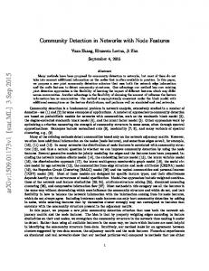
Consider the asymmetrically coupled network of Fig. 2共a兲. The coupling coefficients cij are in general different, but it is easy to check that node balance holds. The corresponding symmetrized network is represented in Fig. 2共b兲. In order to calculate synchronization bounds, we apply the connection graph method to the symmetrized network. We have to choose a path Pij between any pair of nodes i , j. Our choice is

Downloaded 03 Apr 2006 to 131.96.241.65. Redistribution subject to AIP license or copyright, see http://chaos.aip.org/chaos/copyright.jsp

015102-7

Chaos 16, 015102 共2006兲

Synchrony in node balanced networks

4c ⬎

a · 1, 6

5c ⬎

a · 5, 6

5c ⬎

a · 3. 6

The bounds for edges 4, 6, and 7 give the maximum constraint, therefore we conclude that for c⬎

a ⬇ 0.1668a 6

共30兲

we can guarantee global synchronization of the network both for the asymmetrically and symmetrically coupled case. The second largest eigenvalue of the connectivity matrix of the asymmetrically coupled network is calculated numerically = − 10c ␭asym 2 and for its symmetrization ␭sym 2 = − 8.1852c. FIG. 2. 共a兲 Asymmetrically coupled network with node balance. Arrows indicate direction of coupling along an edge. 共b兲 The symmetrized mutually coupled network.

P12:edge 2,

P23:edge 7,

P35:edges 5,8,

P13:edge 1,

P24:edges 7,8,

P36:edge 9,

P14:edge 3,

P25:edges 2,4,

P45:edge 5,

P15:edge 4,

P26:edges 7,9,

P46:edges 5,6,

By the eigenvalue approaches to global synchronization, the synchronization bound associated with the second largest eigenvalue of the connectivity matrix is c ⬎ a/兩Re ␭2兩.

共31兲

Note that this is true only for networks where there is no desynchronization with increasing coupling and the parameter a can be rigorously derived. The condition 共31兲 gives the following upper bound for global synchronization: 兩 = 0.1a c ⬎ a/兩␭asym 2

共32兲

for the asymmetrically coupled, and

P16:edges 4,6,

P34:edge 8,

P56:edge 6.

Now we have to calculate, for each edge k of the graph, the sum of the lengths of all chosen paths Pij passing through k:

兺

bk =

兩共Pij兲兩.

j⬎i;k苸Pij

Here, the path length is the number of edges comprising each Pij. The result is b1 = 1,

b4 = 5,

b7 = 5,

b2 = 3,

b5 = 5,

b8 = 5,

b3 = 1,

b6 = 5,

b9 = 3.

By condition 共27兲, this leads to the constraints to achieve global synchronization: a · 5, 6

4c ⬎

a · 1, 6

5c ⬎

5c ⬎

a · 3, 6

10c ⬎

a · 5, 6

5c ⬎

a · 5, 6

6c ⬎

a · 5, 6

c ⬎ a/兩␭sym 2 兩 = 0.1222a

共33兲

for the symmetrically coupled network. Compared with Eq. 共30兲, this confirms that the connection graph method gives bounds for global synchronization that are not far from the optimal bounds, achievable by the eigenvalue method. The comparison between conditions 共32兲 and 共33兲 shows that the symmetrized network is only slightly more difficult to synchronize than the asymmetrically coupled one. D. Unbalanced nonsynchronizable network

Figure 3共a兲 shows the simplest network that is impossible to synchronize due to its connection structure, i.e., for any individual systems that do not have unique asymptotic behavior, even for arbitrarily large coupling constants c the network cannot achieve synchronization. Indeed, systems 1 and 2 have no interaction at all and therefore they do not synchronize. The symmetrized network 关Fig. 3共b兲兴, however, can easily be seen to synchronize for c ⬎ 2a by applying the connection graph method. This example illustrates that it is in general not possible to apply the synchronization bound of the symmetrized network, when the node balance condition is not satisfied. Indeed, in the networks of Fig. 3 no node achieves node balance.

Downloaded 03 Apr 2006 to 131.96.241.65. Redistribution subject to AIP license or copyright, see http://chaos.aip.org/chaos/copyright.jsp

015102-8

Chaos 16, 015102 共2006兲

Belykh, Belykh, and Hasler

sponding undirected networks are also the same, i.e., if the eigenvalue of the asymmetrical and symmetrical connectivity matrices are the same. In general this is not true, but this is the case for a number of networks with a regular structure. Examples include rings of K-nearest neighbor unidirectionally coupled oscillators 共cf. Sec. IV兲 and locally connected two-dimensional lattices on a torus with a uniformly directed coupling. In all other cases we have numerically examined, the symmetrized network was only slightly more difficult to synchronize than the asymmetrically coupled one.

FIG. 3. 共a兲 Simplest nonsynchronizable network, not satisfying the node balance condition. It shows that node balance is crucial for obtaining the same synchronization behavior as in the symmetrized network. 共b兲 Symmetrized, synchronizable network.

V. CONCLUSIONS

We have extended the connection graph stability method to prove global synchronization in networks of coupled dynamical systems. Previously we assumed symmetrical coupling between individual dynamical systems in the network. Here, we have extended the method to asymmetrically coupled networks that satisfy the node balance condition. This condition requires that the sum of coupling coefficients of all edges directed toward a node is equal to the sum of coupling coefficients of all edges directed away from the node. We showed that for networks with node balance it is sufficient to symmetrize all connections by replacing a unidirectional coupling of strength c by a bidirectional coupling of strength c / 2. The bounds for global synchronization for this symmetrized network then also hold for the original asymmetrical network, when we apply our connection graph stability method. Let us remark once more that the connection graph stability method relies solely on graph theoretical reasoning to derive synchronization bounds, that it allows for timedependent coupling coefficients and that it gives values for the critical values of coupling above which global synchronization is rigorously established. If the node balance condition is not satisfied, the asymmetrically coupled network may have very different synchronization behavior from the symmetrized network. The extension of our method to this most general case is a current research topic. It is customary to discuss synchronization properties of networks in terms of eigenvalues of the connectivity matrix. On the one hand, it allows one to give necessary and sufficient conditions for local synchronization depending on 共usually numerically calculated兲 Lyapunov exponents of the individual systems. On the other hand, we have previously shown that in the case of symmetrically coupled networks, the second largest eigenvalue also allows one to obtain a bound for global synchronization. Actually in the context of our quadratic Lyapunov function this is the optimal bound. For networks with node balance, this carries over to asymmetrically connected networks. We may wonder whether the local synchronization properties of directed networks with node balance and the corre-

ACKNOWLEDGMENTS

We thank Lou Pecora and Stefano Boccaletti for useful discussions. This work was supported in part by the SNSF 共Grant No. 21-6526801兲, the EU Commission 共FP6-NEST Project No. 517133兲, and the RFFI-NWO 共Grant No. 047.011.2004.004兲. S. H. Strogatz, Nature 共London兲 410, 268 共2001兲. W. Gerstner and W. Kistler, Spiking Neuron Models 共Cambridge University Press, Cambridge, 2002兲. 3 C. M. Gray and W. Singer, Proc. Natl. Acad. Sci. U.S.A. 86, 1698 共1989兲; M. Bazhenov, M. Stopfer, M. Rabinovich, R. Huerta, H. D. I. Abarbanel, T. J. Sejnowski, and G. Laurent, Neuron 30, 553 共2001兲; M. R. Mehta, A. K. Lee, and M. A. Wilson, Nature 共London兲 417, 741 共2002兲. 4 L. Fabiny, P. Colet, R. Roy, and D. Lenstra, Phys. Rev. A 47, 4287 共1993兲; S. Yu. Kourtchatov, V. V. Likhanskii, A. P. Naparotovich, F. T. Arecchi, and A. Lapucci, ibid. 52, 4089 共1995兲. 5 D. L. Mills, IEEE Trans. Commun. 39, 1482 共1991兲; D. L. Mills, Comput. Commun. Rev. 24, 16 共1994兲. 6 Y. Kuramoto, in International Symposium on Mathematical Problems in Theoretical Physics, edited by H. Araki, Lecture Notes in Physics Vol. 39 共Springer, Berlin, 1975兲, p. 420. 7 N. Kopell and G. B. Ermentrout, Math. Biosci. 90, 87 共1988兲. 8 S. H. Strogatz and R. E. Mirollo, Physica D 31, 143 共1988兲. 9 H. Fujisaka and T. Yamada, Prog. Theor. Phys. 69, 32 共1983兲; 72, 885 共1984兲. 10 V. S. Afraimovich, N. N. Verichev, and M. I. Rabinovich, Radiophys. Quantum Electron. 29, 795 共1986兲. 11 L. M. Pecora and T. L. Carroll, Phys. Rev. Lett. 64, 821 共1990兲. 12 I. Belykh, E. de Lange, and M. Hasler, Phys. Rev. Lett. 94, 188101 共2005兲. 13 J. Kurths, S. Boccaletti, C. Grebogi, and Y.-C. Lai, editors, “Focus issue: Control and synchronization in chaotic dynamical systems,” Chaos 13, 126 共2003兲. 14 V. N. Belykh, N. N. Verichev, L. J. Kocarev, and L. O. Chua, in Chua’s Circuit: A Paradigm for Chaos, edited by R. N. Madan 共World Scientific, Singapore, 1993兲, p. 325. 15 J. F. Heagy, T. L. Carroll, and L. M. Pecora, Phys. Rev. E 50, 1874 共1994兲. 16 C. W. Wu and L. O. Chua, IEEE Trans. Circuits Syst., I: Fundam. Theory Appl. 43, 161 共1996兲. 17 L. M. Pecora, T. L. Carroll, G. A. Johnson, D. J. Mar, and J. F. Heagy, Chaos 7, 520 共1997兲. 18 R. Brown and N. F. Rulkov, Chaos 7, 395 共1997兲. 19 L. M. Pecora and T. L Carroll, Phys. Rev. Lett. 80, 2109 共1998兲. 20 L. M. Pecora, Phys. Rev. E 58, 347 共1998兲. 21 K. S. Fink, G. Johnson, T. Carroll, D. Mar, and L. M. Pecora, Phys. Rev. E 61, 5080 共2000兲. 22 J. Jost and M. P. Joy, Phys. Rev. E 65, 016201 共2001兲. 23 Y. Chen, G. Rangarajan, and M. Ding, Phys. Rev. E 67, 026209 共2003兲. 24 X. F. Wang and G. Chen, IEEE Trans. Circuits Syst., I: Fundam. Theory Appl. 49, 54 共2002兲. 25 V. N Belykh, I. V Belykh, and M. Hasler, Physica D 195, 159 共2004兲. 26 I. V Belykh, V. N. Belykh, and M. Hasler, Physica D 195, 188 共2004兲. 27 I. Belykh, M. Hasler, M. Lauret, and H. Nijmeijer, Int. J. Bifurcation Chaos Appl. Sci. Eng. 15 共2005兲 共in press兲. 1 2

Downloaded 03 Apr 2006 to 131.96.241.65. Redistribution subject to AIP license or copyright, see http://chaos.aip.org/chaos/copyright.jsp

015102-9

M. Barahona and L. M. Pecora, Phys. Rev. Lett. 89, 054101 共2002兲. T. Nishikawa, A. E. Motter, Y.-C. Lai, and F. C. Hoppensteadt, Phys. Rev. Lett. 91, 014101 共2003兲. 30 A. E. Motter, C. Zhou, and J. Kurths, Phys. Rev. E 71, 016116 共2005兲. 31 D. U. Hwang, M. Chavez, A. Amann, and S. Boccaletti, Phys. Rev. Lett. 94, 138701 共2005兲. 32 M. Chavez, D. U. Hwang, A. Amann, and S. Boccaletti, Phys. Rev. Lett. 94, 218701 共2005兲. 28 29

Chaos 16, 015102 共2006兲

Synchrony in node balanced networks 33

A. Yu. Pogromsky and H. Nijmeijer, IEEE Trans. Circuits Syst., I: Fundam. Theory Appl. 48, 152 共2001兲. 34 C. W. Wu, Synchronization in Coupled Chaotic Circuits and Systems, World Scientific Series on Nonlinear Science, Series A Vol. 41 共World Scientific, Singapore, 2002兲. 35 C. W. Wu, Nonlinearity 18, 1057 共2005兲. 36 I. V. Belykh, V. N. Belykh, K. V. Nevidin, and M. Hasler, Chaos 13, 165 共2003兲.

Downloaded 03 Apr 2006 to 131.96.241.65. Redistribution subject to AIP license or copyright, see http://chaos.aip.org/chaos/copyright.jsp