cycle van der Pol oscillator and, chaotic Rössler and Lorenz systems. Stability ... chaotic oscillators and, mixed synchronization are given in electronic circuits.
Synchronization in counter-rotating oscillators Sourav K. Bhowmick1, Dibakar Ghosh2, Syamal K. Dana1 1
Central Instrumentation, Indian Institute of Chemical Biology (Council of Scientific and Industrial Research) Jadavpur, Kolkata 700032, India 2 Department of Mathematics, Dinabandhu Andrews College, Kolkata 700084, India. An oscillatory system can have opposite senses of rotation, clockwise or anticlockwise. We present a general mathematical description how to obtain counter-rotating oscillators from the definition of a dynamical system. A type of mixed synchronization emerges in counter-rotating oscillators under diffusive scalar coupling when complete synchronization and antisynchronization coexist in different state variables. We present numerical examples of limit cycle van der Pol oscillator and, chaotic Rössler and Lorenz systems. Stability conditions of mixed synchronization are analytically obtained for both Rössler and Lorenz systems. Experimental evidences of counter-rotating limit cycle and chaotic oscillators and, mixed synchronization are given in electronic circuits. PACS numbers: 05.45.Xt, 05.45.Gg
Counter-rotating vortices coexist in a fluid medium, atmosphere and ocean, which destroy each other when they collide and reborn if the interaction is withdrawn. Attempts are found in literature to explain such spatiotemporal behaviors and their instabilities. On the other hand, counter-rotating vortices are created in physical systems, plasma flow and Bose-Einstein condensates, for useful purposes. The trajectory of nonlinear dynamical systems too shows opposite senses of rotation, clockwise and anticlockwise direction. A question naturally arises how counter-rotating vortices or oscillators are created and interact with each other. These issues are not well understood. We make an attempt to address the questions here, however, restricting our interest to the simpler cases of nonlinear dynamical systems. In studies of nonlinear oscillators, all oscillators are assumed to rotate in same direction, either clockwise or anticlockwise. These corotating oscillators when interact through coupling emerge into a synchronization regime where all the state variables follow one and unique correlation rule, complete synchronization or antisynchronization. In contrast, counter-rotating oscillators under diffusive coupling show emergence of an uncommon type of synchronization defined as mixed synchronization. In this synchronization regime, some of the state variables emerge into complete synchronization while others are in antisynchronization. We try to understand here the underlying principle how counter-rotating oscillators are created from a known dynamical system and then derive the stability condition of mixed synchronization. We construct counter-rotating oscillators in electronic circuits to evidence mixed synchronization.
I. Introduction Synchronization is well investigated [1] in oscillatory systems, limit cycle as well as chaotic. The nature and strength of coupling decides the type of synchronization, either in both amplitude and phase [1-2] or only in phase [1, 3]. The emergent phase correlation in the coupled oscillators may be in-phase or antiphase. However, the sense of rotation of the trajectories of the interacting oscillators in these studies is
always assumed same. This class of co-rotating oscillators emerge into a kind of coherent state, as example, complete synchronization (CS) or antisynchronization (AS). All the state variables follow same type of correlation, CS or AS. On the other hand, a recent study [4] revealed that the sense of rotation of the trajectory of a dynamical system may be clockwise or anticlockwise. Apparently, this sounds trivial and the topic remained ignored so far. But it is very nontrivial [4] that such counter-rotating oscillators under diffusive coupling emerge into a different type of correlation. The state variables of the coupled counter-rotating oscillators emerge into a mixed synchronization (MS) where a pair of state variables develops a CS state while another pair is in a AS state. It is true that existence of a MS state was reported earlier [5] in coupled corotating Lorenz systems for a specific scalar coupling. This emergent MS state has justification in the inherent axial symmetry of the Lorenz system but it was not observed, to our best knowledge, in other systems under linear diffusive coupling. However, a design of coupling was proposed [6] for engineering a MS state in co-rotating oscillators. In contrast, in counter-rotating oscillators, the MS state emerges naturally under diffusive scalar coupling. This observation encourages further investigation to understand the origin of counterrotating oscillators and related coupled dynamics. In fact, counter-rotating vortices (CRV) are the key elements of dynamical atmosphere and ocean [7]. They coexist in a fluid medium which destroy each other when they collide and reborn if the interaction is withdrawn. How a CRV pair is created? How they interact with each other? These are important questions necessitate appropriate answer for reducing damage of an aircraft, since CRV pair originates in the wake of an aircraft during take-off and landing [8]. On the other hand, counter-rotating vortices are deliberately created in physical systems, magnetohydrodynamics of plasma flow [9], Bose-Einstein condensates [10] for useful purposes. Counterrotating spirals are also seen in biological medium such as protoplasm of the Physarum plasmodium [11]. All these facts strongly suggest that counter-rotating time evolving dynamical systems may exist in nature and may have beneficial role to play. From these viewpoints, it demands a special attention and a possible revision of the existing knowledge of synchronization, particularly, in context of collective behaviors of a network of a mixed population of counter-
rotating oscillators. Presently, we restrict our study to a simpler case of two counter-rotating oscillators. The existence of clockwise and counter-clockwise rotation in a dynamical system was noticed by Tabor [12] in relation to rotation of a 2D limit cycle system near the Hopf bifurcation point. However, the variation of rotational direction was not considered while investigating collective dynamics of oscillators until recently [4]. The study made an extension to chaotic oscillators. Any general statement was still missing how to induce counter-rotation and to explain the mechanism of counter-rotation in a known dynamical system. We present a general mathematical description, in this paper, how to create counter-rotating motion in a given dynamical system, limit cycle or chaotic, and then investigate the collective behavior. A particular type of MS regime emerges in pairs of state variables for different choices of scalar coupling. We analytically established the stability conditions of MS for coupled chaotic systems. We tested our proposition using numerical simulations of limit cycle as well as chaotic system. Finally, we supported the numerical results with experiments by constructing electronic circuits of counter-rotating van der Pol and piecewise Rössler oscillators. The rest of the paper is organized as follows: theory of counter-rotating oscillators is presented in section II with examples in section IIA. Mixed synchronization in van der Pol oscillator [13], chaotic Rössler oscillator [14] and Lorenz systems [15] is described in section III. The stability condition of MS in the chaotic systems are described in section IV. Experimental evidences of counter-rotating oscillators and MS regime is described in V with a conclusion in section VI. II. Counter rotating oscillators: Method A dynamical system can always be expressed by, X� = AX + f ( X ) + C
(1)
where X ∈ R n is a state vector, A is a n × n constant matrix and represents the linear part of the system, f : R n → R n contains the nonlinear part of the system and, C is a n × 1 constant matrix. For a 3D system when A=(aij)3×3 and X=[x, y, z]T, a general procedure is stated in the following steps for deriving counter-rotating oscillators. Crucial changes are made in the A matrix, i.e., in the linear part of the system, i) there must exist at least one pair of non-zero conjugate elements a ij , a ji , i ≠ j in the matrix A,
trajectory can be flipped [4] by altering the sign of the conjugate pair of elements of the A matrix. This is as usually done in case of quantum rotation [10] by changing the sign of the angular frequency. This can be extended to frame a general rule following the standard Eurler’s rotation theorem [16]. In a 3D system, as stated in the Euler’s rotation theorem, any rotation can be described using three angles of rotation around three coordinate axes. The final rotation matrix is a product of three rotational matrices and given by, ⎡a11 ⎢ A= ⎢a 21 ⎢⎣a31
a12 a 22
a13 ⎤ ⎥ a 23 ⎥ a33 ⎥⎦
(2)
a32 where a11= cos ϕ cos κ ; a12= cos ω sin κ + sin ω sin ϕ cos κ a13= sin ω sin κ − cos ω sin ϕ cos κ a21= − cos ϕ sin κ ; a22= cos ω cos κ − sin ω sin ϕ sin κ
a23= sin ω cos κ + cos ω sin ϕ sin κ a31= sin ϕ ; a32= − sin ω cos ϕ ; a33= cos ω cos ϕ and κ , ϕ , ω are the rotation angles in any of the 2D coordinate spaces around the remaining third coordinate. Suppose we consider the x-y plane of rotation around the z-axis then the rotation angle is κ ( ω = 0, ϕ = 0 ): the new co-ordinate (x1, y1, z1) of the point (x, y, z) after rotation by the angle κ is written, ⎡ x1 ⎤ ⎡ cos κ ⎢ y ⎥ = ⎢− sin κ ⎢ 1⎥ ⎢ ⎣⎢ z1 ⎦⎥ ⎣⎢ 0
sin κ cos κ 0
0⎤ ⎡ x ⎤ 0⎥⎥ ⎢⎢ y ⎥⎥ 1⎦⎥ ⎣⎢ z ⎦⎥
(3)
The direction of rotation will reverse if the rotation angle κ is taken as negative i.e., if κ is substituted by -κ. The transformed coordinate (x2, y2, z2) in reverse direction is, ⎡ x 2 ⎤ ⎡cos κ ⎢ ⎥ ⎢ ⎢ y 2 ⎥ = ⎢ sin κ ⎢⎣ z 2 ⎥⎦ ⎢⎣ 0
− sin κ cos κ 0
0⎤ ⎡ x ⎤ ⎥⎢ ⎥ 0⎥ ⎢ y ⎥ 1 ⎥⎦ ⎢⎣ z ⎥⎦
(4)
A change of sign of the elements a12 , a21 in (4) is thus needed to induce a change in the direction of rotation in the x-y plane in respect of the z-direction. The counter-rotation in the y-z plane in respect to the x-axis is obtained, ω ≠0 ( κ = 0, ϕ = 0 ),
where i, j=1,2,3. ii)
then replace the element aij by − aij (i ≠ j ) or
vice versa. The clockwise or anticlockwise rotation of the trajectory of a 3D dynamical system is described as the direction of rotation of the trajectory in a 2D plane in respect to the third coordinate. As stated in (ii), the sense of rotation of a
0 ⎡ x1 ⎤ ⎡1 ⎢ ⎥ ⎢ ⎢ y1 ⎥ = ⎢0 cos ω ⎢⎣ z1 ⎥⎦ ⎢⎣0 − sin ω
0 ⎤⎡ x⎤ ⎥⎢ ⎥ sin ω ⎥ ⎢ y ⎥ cos ω ⎥⎦ ⎢⎣ z ⎥⎦
(5)
The sign of the elements a23 and a32 of the A matrix are to be exchanged for counter-rotation in the y-z plane with respect to the x-axis. Similarly, we can derive a rotation matrix for
rotation angle ϕ≠0 ( κ = 0, ω = 0 ) in the x-z plane around the y-axis and accordingly introduce an exchange sign in a13 and a31 elements to obtain counter-rotation. The general matrix (2) is thus obtained by multiplication of the three rotational matrices for three angles of rotation, ω , ϕ , κ . We consider only one axis of counter-rotation for our application and hence suffice to use (3) for our studies. We elaborate this with real examples of dynamical systems.
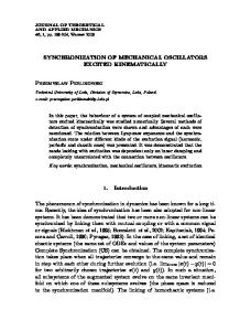
model in the upper panels is the x-y plane for opposite signs of a12 and a21 elements in the linear matrix of (6). While in Sprott system in the lower panels, it is the x-z plane when the a13 and a31 elements of the linear matrix of (7) are altered. Noteworthy that two largest Lyapunov exponents of two oscillators before coupling are almost same [4] for ω1 = 1 and ω 2 = −1 . Note that, in addition to changes in the sense of rotation, there is a change in the position of the attractors in phase space (Fig.1).
IIA. Counter rotating oscillators: Examples III. Synchronization of counter-rotating oscillators Here we describe examples of counter-rotating oscillators, (1) Chua oscillator [17] x� i = a( xi − ω i yi − g ( xi )), y� i = b(ω i xi − yi + z i ) z�i = −cyi
(6)
g ( xi ) = m1 xi + m1 − m0 if xi ≤ −1
where
= m0 xi
if - 1 ≤ xi ≤ 1 and
= m1 xi − m0 - m1 if 1 ≤ xi
We consider two coupled counter-rotating oscillators to explore synchronization, x� = Ax + f ( x ) + C + HG ( y , x) y� = A′y + f ( y ) + C + HG ( x, y )
(9)
where x=[x1 y1 z1]T, y =[x2 y2 z2]T are the state vectors, A and A΄ are the linear matrices for counter-rotating oscillators and, H=diag(ε1, ε2, ε3) is the coupling matrix,
a = 15.6, b = 1, c = 33, m0 = -8/7, m1 = -5/7, i=1,2, and ω1=1, ω2=-1. (2) Sprott system [18] x� i = xi yi − ω i z i , y� i = xi − yi z�i = ω i xi + 0.3 z i
(8)
and
⎡ x1 − x 2 ⎤ G ( x, y ) = ⎢⎢ y1 − y 2 ⎥⎥ . ⎢⎣ z1 − z 2 ⎥⎦
(7)
where i=1, 2 and ω1=1, ω2=-1
When two counter-rotating oscillators are coupled in a scalar mode, a MS state emerges above a critical coupling. The scalar coupling must use at least one of the pairs of variables from the plane of rotation (x-y plane), either the pair of x1-x2 variables (ε1=ε, ε2=0, ε3=0) or the pair of y1-y2 variables (ε1=0 ε2=ε, ε3=0) of the coupled oscillators. Alternatively, if one oscillator is rotating clockwise in the x1-z1 plane and another in anticlockwise direction in the x2-z2 plane, either of the couplings, (ε1=ε, ε2=0, ε3=0) and (ε1=0, ε2=0, ε3=ε), can be used for MS and so on. We elaborate first using a limit cycle van der Pol oscillator, x�1 = y1 , y�1 = b(1 − x12 ) y1 − x1
(10)
where b is the only parameter. The linear matrix of (10) for clockwise rotation is given by A and a counter-clockwise rotation is derived by replacing it with A′ ,
Fig.1. Phase portraits of counter-rotating oscillators. Chua system (6) in upper two panels, and Sprott system (7) in lower two panels.
Phase portraits of counter-rotating Chua oscillator and a Sprott system are shown in Fig.1. Clearly by changing the sign of a conjugate pair of elements in the linear matrices of the systems, a counter-rotation in the trajectories of the dynamical systems are induced. Note that the rotational plane of the Chua
⎡0 − 1⎤ ⎡ 0 1⎤ ; (11) A′ = ⎢ A=⎢ ⎥ ⎥ ⎣1 b ⎦ ⎣− 1 b ⎦ Two counter-rotating van der Pol oscillators under a scalar diffusive coupling are,
x� i = ω i y i + ε ( x j − x i );
y� i = b(1 − x i2 ) y i − ω i x i
(12)
where i, j=1,2 and ω1=1, ω2=-1, ε is the coupling strength.
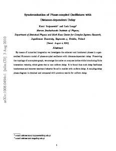
Numerically simulated phase portraits show two isolated counter-rotating oscillators in Fig.2(a) and 2(b) where the rotation of the trajectory is made opposite in the x-y plane by changing the sign of ω1. As stated above, a MS state only emerges in two different state variables as shown in Fig.2(c) and 2(d). The x1 vs. x2 plot confirms a CS state when x1 and x2 are only directly coupled while y1vs. y2 shows an AS state. The coupling has a critical value for a choice of system parameter b as shown in a phase diagram in Fig.2(e). The boundary of the MS state in a shaded region and nonsynchronization in the white region is the critical coupling.
which is chaotic for a=b=0.2, c=10, ω1=1. The linear matrices of the Rössler model for counter-rotations, ⎡0 A= ⎢ω ⎢ 1 ⎢⎣ 0
− ω1 a 0
− 1⎤ 0 ⎥⎥ ; c ⎥⎦
ω1 ⎡ 0 ⎢ ′ A = ⎢ − ω1 a ⎢⎣ 0 0
− 1⎤ 0 ⎥⎥ c ⎥⎦
(14)
where the sign of the a12, a21 elements in the linear matrix A are altered. The counter-rotating Rössler oscillators after coupling via a single variable or scalar coupling is
x� i = −ω i y i − z i + ε ( x j − xi ) y� i = ω i xi + ay i z� i = b + z i ( x i − c)
(15)
where i=1, 2 represents two oscillators, ω1 = 1, ω 2 = −1 and ε is the coupling strength as usual. Phase portraits of counterrotating Rössler oscillators before coupling are shown in Figs.3(a) and 3(b). For scalar diffusive coupling, a MS state emerges for ε≥εc, a critical coupling. To realize MS, the oscillators must be coupled at least by one of the state variables involved in the plane of rotation. As described above, CS is noticed in that pair of variables which are directly coupled, and AS in the other pair of variables those are not directly coupled in the rotational plane. The coupling of the counter-rotating Rössler oscillators is made via x-variables, hence x-variables are in a CS state and y-variables (since the plane of rotation is x-y) are in an AS state. The third variables z1-z2 are in a CS state (not shown here). This third pair of variables may be in CS or AS state, which is arbitrarily decided and not clearly understood so far. However it depends upon the system’s inherent property too as found [5] in case of co-rotating Lorenz systems.
Synchronization
(e)
Fig 2: Counter-rotating van der Pol oscillators, b=2.0. Phase portraits of uncoupled van der Pol oscillators, (a) linear matrix A, (b) linear matrix A ′ . MS for ε=0.075, (c) CS, x1vs.x2, (d) AS, y1vs..y2. Phase diagram in ε-b plane showing MS boundary in (e).
Next we use the Rössler oscillator and the Lorenz oscillator to elaborate counter-rotating chaotic systems and their MS behavior. As a first example, we consider the Rössler oscillator,
x� = −ω1 y − z, y� = ω1 x + ay, z� = b + z ( x − c)
(13)
Fig.3. Counter-rotating Rössler oscillators: (a) linear matrix A, (b) linear matrix A’, (c) CS in x1-x2 and, (d) AS in y1-y2. Coupling strength, ε = 0.15 .
Next, we consider the second example of two coupled counterrotating Lorenz systems, x�i = σ (ωi yi − xi ), y�i = ωi r xi − yi − xi zi + ε ( y j − yi )
z�i = xi yi − bzi
(16)
where σ=10, r=28, b=8/3 and, i , j = 1, 2 ; ω1=1, ω2=-1. The linear matrices for counter-rotations of the isolated Lorenz system are A and A΄, ⎡− σ A = ⎢⎢ r ⎢⎣ 0
0⎤ ⎡− σ ⎥ and ′ A = ⎢⎢ − r −1 0 ⎥ ⎢⎣ 0 0 − b⎥⎦
σ
−σ −1 0
0⎤ 0 ⎥⎥ − b ⎥⎦
Let η1 and η2 represent the deviation from a synchronized state, their dynamics is governed by linear equations
η�1 = Aη1 + f ′( x)η1 + H (η2 − η1) η�2 = A′η2 + f ′( y )η2 + H (η1 − η2 )
(18) (19)
It is very difficult to analyze the stability of the system (18)(19) and hence make an approximation [20] by taking time average of the Jacobians, f ′( x ) and f ′( y ) and replacing them by a constant λ . For MS in counter-rotating systems, x=±y (CS or AS ), let η=η1−η2,
(17)
η� = Aη + λη − 2Hη = [ A + λI 3 − 2H]η
(20)
η=0 will be stable if P=A +λΙ3-2H2λ+a and 2ε