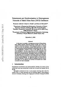
May 31, 2018 - [17] Maurizio Porfiri and Daniel J Stilwell, Consensus seek- ing over random .... [42] Nancy Kopell and Bard Ermentrout, Chemical and elec-.
Synchronization in multilayer networks: when good links go bad Igor Belykh, Douglas Carter Jr., and Russell Jeter
Department of Mathematics and Statistics and Neuroscience Institute, Georgia State University, P.O. Box 4110, Atlanta, Georgia, 30302-410, USA (Dated: May 31, 2018)
Many complex biological and technological systems can be represented by multilayer networks where the nodes are coupled via several independent networks. Despite its signi�cance from both the theoretical and application perspectives, synchronization in multilayer networks and its dependence on the network topology remain poorly understood.
In this paper, we develop a universal
connection graph-based method which removes a long-standing obstacle to studying synchronization in dynamical multilayer networks. This method opens up the possibility of explicitly assessing critical multilayer-induced interactions which can hamper network synchronization and reveals striking, counterintuitive e�ects caused by multilayer coupling.
It demonstrates that a coupling which is
favorable to synchronization in single-layer networks can reverse its role and destabilize synchronization when used in a multilayer network.
This property is controlled by the tra�c load on a
given edge when the replacement of a lightly loaded edge in one layer with a coupling from another layer can promote synchronization, but a similar replacement of a highly loaded edge can break synchronization, forcing a �good� link go �bad.� This method can be transformative in the highly active research �eld of synchronization in multilayer engineering and social networks, especially in regard to hidden e�ects not seen in single-layer networks. PACS numbers: 05.45.Xt, 87.19.La
I.
INTRODUCTION
connectivity.
Multilayer-induced correlations can have
signi�cant rami�cations for the dynamical processes on Complex networks are common models for many systems in physics, biology, engineering, and the social sciences [1�3].
Signi�cant attention has been devoted to
algebraic, statistical, and graph theoretical properties of networks and their relationship to network dynamics (see a review [4] and references therein). The strongest form of network cooperative dynamics is synchronization which has been shown to play an important role in the functioning of a wide spectrum of technological and biological networks [5�14], including adaptive and evolving networks [15�22].
networks, including the e�ects on the speed of disease transmission in social networks [51] and the role of redundant interdependencies on the robustness of multiplex networks to failure [52]. Typically, in single-layer networks of continuous time oscillators, synchronization becomes stable when the coupling strength between the oscillators exceeds a threshold value [23, 30]. This threshold depends on the individual oscillator dynamics and the network topology.
In this
context, a central question is to determine the critical coupling strength so that the stability of synchronization is guaranteed. The master stability function [23] or
Despite the vast literature to be found on network
the connection graph method [30, 31] are usually used
dynamics and synchronization, the majority of research
to answer this question in single-layer networks.
activities have been focused on oscillators connected
methods reduce the dimensionality of the problem such
Both
through single-layer network (one type of coupling) [23�
that synchronization in a large, complex network can be
41]. However, in many realistic biological and engineer-
predicted from the dynamics of the individual node and
ing systems the units can be coupled via multiple, in-
the network structure.
dependent systems and networks. Neurons are typically
Synchronization in multilayer networks has been stud-
connected through di�erent types of couplings such as
ied in [53�56]; however, its critical properties and ex-
excitatory, inhibitory, and electrical synapses, each cor-
plicit dependence on intralayer and interlayer network
responding to a di�erent circuitry whose interplay a�ects
structures remain poorly understood. This is in particu-
network function [42, 43]. Pedestrians on a lively bridge
lar due to the inability of the existing eigenvalue meth-
are coupled via several layers of communication, includ-
ods, including the master stability function [23] to give
ing people-to-people interactions and a feedback from the
detailed insight into the stability condition of synchro-
bridge that can lead to complex pedestrian-bridge dy-
nization as the eigenvalues, corresponding to connection
namics [44�47]. In engineering systems, examples of inde-
graphs composing a multilayer network, must be calcu-
pendent networks include coupled grids of power stations
lated via simultaneous diagonalization of two or more
and communication servers where the failure of nodes in
connectivity matrices.
one network may lead to the failure of dependent nodes
two or more matrices is impossible in general, unless the
in another network [48].
matrices commute [53, 54].
Such interconnected networks
Simultaneous diagonalization of A nice approach based on
can be represented as multiplex or multilayer networks
simultaneous block diagonalization of two connectivity
[49, 50] which include multiple systems and layers of
matrices was proposed in [54]. This most successful ap-
2
plication of the eigenvalue-based approach allows one to
II.
NETWORK MODEL AND PROBLEM STATEMENT
reduce the dimensionality of a large network to a smaller network whose synchronization condition can be used to evaluate the stability of synchronization in the large network. For some network topologies, this technique yields a substantial reduction of the dimensionality; however, this reduction is less signi�cant in general. The reduced network typically contains weighted positive and negative connections, including self loops such that the role of multilayer network topologies and the location of an edge remain di�cult to evaluate. In this paper, we report our signi�cant progress towards removing this long-standing obstacle to studying synchronization in multilayer networks. We develop a new general stability approach, called the Multilayer Connection Graph method, which does not depend on explicit knowledge of the spectrum of the connectivity matrices and can handle multilayer networks with arbitrary network topologies, which are out of reach for the existing approaches. An example of a multilayer network in this study is a network of Lorenz systems where some of the oscillators are coupled through the layer), some through the
y
x variable (�rst
variable (second layer), and
some through both (interlayer connections). Our Multilayer Connection Graph method originates from the connection graph method [30, 31] for single-layer networks; however, this extension is highly non-trivial and requires overcoming a number of technically challenging issues. This includes the fact that the oscillators from two
y
x and
layers in the networks of Lorenz systems are connected
through the intrinsic, nonlinear equations of the Lorenz system. As a result, multilayer networks can have drastically di�erent synchronization properties from those of single-layer networks.
In particular, our method shows
that an interlayer tra�c load on a link is the crucial quantity which can be used to foster or hamper synchronization in a nonlinear fashion. For example, it demonstrates that replacing a link with a light interlayer tra�c load by a stronger pairwise converging coupling (a �good� link) via another layer may lower the synchronization threshold and improve synchronizability.
At the same time,
such a replacement of a highly loaded link can make the network unsynchronizable, forcing the pairwise stabilizing �good� link go �bad.�
We start with a general network of
n
oscillators with
two connectivity layers:
n n X X dxi = F(xi ) + cij P xj + dij Lxj , i = 1, ..., n, dt j=1 j=1
(1)
xi = (x1i , ..., xsi ) is the s state vector containing the i-th oscillator, F : Rs → Rs describes the oscillators' individual dynamics, cij and dij are the coupling strengths. C = (cij ) and D = (dij ) are n × n where
coordinates of the
Laplacian connectivity matrices with zero-row sums and nonnegative o�-diagonal elements
cij = cji
and
respectively [30]. These connectivity matrices
dij = dji , C and D
de�ne two di�erent connection layers (also denoted by
C
and
D,
with
ner matrices
P
m
and
and
L
l
edges, respectively).
The in-
determine which variables couple
the oscillators within the
C
and
D
layers, respectively.
Without loss of generality, we will be considering the os-
xi = (xi , yi , zi ). ThereP = diag(1, 0, 0) will correspond to the �rst-layer connections via x, while the D graph with the inner matrix L = diag(0, 1, 0 ) will indicate the second-layer connections via y. Overall, the
cillators of dimension fore, the
C
s=3
and
graph with the inner matrix
oscillators of the network are connected through a combination of the two layers (see Fig. 1 for an example of a combined two-layer graph). The graphs are assumed to be undirected [30]. Oscillators, comprising the network (1), can be periodic or chaotic. As chaotic oscillators are di�cult to synchronize, they are usually used as test bed examples for probing the e�ectiveness of a given stability approach. The oscillators used in the numerical veri�cation of our stability method are chaotic Lorenz [57] and double scroll oscillators [58]. In this paper, we are interested in the stability of complete synchronization de�ned by the synchronization manifold
M = {x1 = x2 = ... = xn }.
Our main objec-
tive is to determine a threshold value for the coupling strengths required for the global stability of synchronization.
We seek to predict this threshold or the absence
thereof in the general network (1) from synchronization in the simplest two-node network and graph properties
The layout of this paper is as follows.
First, in Sec.
of the two-layer network structures.
In Sec.
It is important to emphasize that only Type I oscilla-
III, we start with a motivating example of why the re-
tors [26] are capable of synchronizing globally and retain-
placement of some links in a multilayer network can im-
ing synchronization for any coupling strengths exceeding
prove or break network synchronization.
the synchronization threshold.
II, we present and discuss the network model.
And what is
Most known oscillators,
IV, we formulate
including the Lorenz and double scroll oscillators belong
the Multilayer Connection Graph method for predicting
to Type I systems. A much more narrow Type II class
synchronization in multilayer networks. In Secs. V and
of oscillators contains
VI, we show how to apply the general method to speci�c
which synchronization becomes only locally stable and
network topologies. In Sec. VII, a brief discussion of the
eventually looses its stability with an increase of cou-
obtained results is given. Finally, the Appendix contains
pling [24].
the complete derivation of the general method.
MAT-
Type I networks in this paper; however, a numerically-
LAB code for algorithms used for calculating network
assisted extension of our method to Type II networks can
tra�c loads are given in the Supplement.
be performed with moderate e�ort and remains a subject
an underlying mechanism?
In Sec.
x-coupled
Rössler systems [23] in
As a result, we limit our consideration to
3
of future study.
tering or hindering synchronization, we begin with twolayer networks of chaotic Lorenz oscillators, depicted in
(a)
Fig. 1(a-c). For the Lorenz oscillators, the vector equation (1) can be written in a more reader-friendly scalar form:
n P
x˙ i = σ(yi − xi ) +
cij xj ,
j=1
(b)
n P
y˙ i = rxi − yi − xi zi +
(2)
dij yj ,
j=1
z˙i = −bzi + xi yi , i = 1, ..., n, C = (cij ) describes the x connections (black edges in Fig. 1(a-c)), D = (dij ) describes the location of one y
where the connectivity matrix topology of
(c)
and matrix
edge (blue or red edge). The parameters of the individ-
σ = 10, r = 28, and b = 8/3. The strengths of the x and y coupling are homogeneous (cij = c, dij = d) and varied uniformly (c = d).
ual Lorenz oscillator are standard:
(d)
We are interested in the question of how the replacement of an
x
y
edge in the network of Fig. 1(a) with a
edge can a�ect synchronization.
To address this ques-
tion, we �rst need to understand synchronization properties of two-node single-layer networks of
y -coupled
Lorenz systems.
x-coupled and
It is well-known that if the
coupling in a single-layer network (2) with either all all
y
x
or
connections exceeds a critical threshold, then syn-
c > c∗ d > d∗ , respectively. A rigorous upper bound for the ∗ critical coupling c , explicit in parameters of the Lorenz chronization becomes stable and persists for any
and
oscillator can be found in [30]. Calculated numerically, these coupling thresholds are
c∗ ≈ 3.81 d∗ ≈ 1.42 for
x-coupled network and y -coupled network. As the synchro∗ nization threshold d is signi�cantly lower, then one could expect that replacing an x edge with a presumably better converging y coupling improves synchronization. This is true for the network of Fig. 1(b) when x edge 5-6 is replaced with a y edge, yielding a minor reduction in the ∗ synchronization threshold from c ≈ 17.94 in the single∗ layer x-coupled network of Fig. 1(a) to c ≈ 17.74 in
for
FIG. 1.
The puzzle:
why do �good� links go �bad�?
Syn-
chronization in six-node networks of Lorenz systems (2). (a) Single-layer network, with all placement of ing
y
x
edge
5-6
x
edges (black).
(b) The re-
with a presumably better converg-
coupling (blue) improves synchronization, as expected
(see (d)). (c) A similar replacement of
x
edge
2-3
with a
y
edge (red) makes synchronization impossible by pushing the threshold to in�nity (see (d)). (d). Systematic study of the ∗ coupling threshold c as a function of the y edge location that replaces an
x
edge in the original
x-coupled
network (a).
The blue solid line indicates numerically calculated threshint olds. The black solid line depicts the interlayer tra�c b for int the respective y edge. Note a signi�cant increase of b that causes the network to become unsynchronizable as predicted by the method. The predicted coupling thresholds (blue dotted line) are computed from (3) using the exponential �t in Fig. 3 and scaling factors
β = 0.18
and
γ = 0.7180.
for the two-node the
the multilayer network of Fig. 1(b).
A surprise comes
from the network of Fig. 1(c) where the replacement of
x edge with a y
edge, that would be expected to improve
synchronization, on the contrary makes the network unsynchronizable (see the coupling threshold jumping to in�nity in Fig. 1(d)). What is the origin of this highly counterintuitive e�ect? Why do edges in a multilayer network reverse their stabilizing roles depending on the edge location whereas they are well behaved in single-layer networks? nectivity matrices for
x
and
y
As the con-
coupling in the networks
of Fig. 1(b) and Fig. 1(c) do not commute and, therefore, the predictive power of the master stability function III.
A MOTIVATING EXAMPLE AND A PUZZLE
based methods [53�55] is severely impaired, this puzzle calls for an explanation and utlimately motivates the development of an e�ective, general method for assessing
To illustrate the complexity of assessing the role of multilayer connections and their controversial role in fos-
the stability of synchronization in multilayer networks. In the following, we will develop such a method that
4
identi�es the location of critical interlayer links which
is given in the Appendix.
control stable synchronization and reveals its explicit de-
Remark 1.
pendence on an interlayer tra�c load on a given edge.
oretical quantities
�
In terms of tra�c networks, the graph the-
bxk , byk
and
bint k
represent the total
lengths of the chosen roads that go through a given edge
k
which can be loosely analogized as a busy street. ThereIV.
MULTILAYER CONNECTION GRAPH
fore, we refer to them as �tra�c� loads. In this view, the
METHOD
quantity
bint k
is a tra�c load on edge
k,
caused by in-
terlayer travelers. It is important to notice that positive In this section, we �rst present the main result of this
terms
+ωx bint k LXk
in the equation (4) and
+ωy bint k P Xk
paper and formulate the method. We will then demon-
in (5) play a destabilizing role such that a heavily loaded
strate how to apply the method to speci�c network con-
edge with a high
�gurations.
for making the systems (4) and (5) stable at all. This ob-
Theorem 1 [The method].
servation has dramatic consequences for synchronization
Synchronization in the multilayer network (1) is globally stable if for each edge k = 1, ..., m (l)
in speci�c multilayer networks described in the following
n P
|Pij |
j>i; k∈Pij ∈C
Remark 2. (3)
is the sum of the lengths
of all chosen paths Pij between any pair of oscillators i and j which belong to the x graph C and go through a given x edge. The path length |Pij | is the number of edges comprising the path. Similarly, byk corresponds to the sum of the lengths of all chosen paths which belong to the y graph D and go through a given y edge. bint is k the sum of the lengths of all chosen paths which contain x and y edges and belong to the combined, two-layer xy graph and go through a given edge k which may be an x or y edge. Constant ax (ay ) is the double coupling strength su�cient for synchronization in the network of two xcoupled (y-coupled) oscillators, composing the network. The constants ωx and ωy represent a combination of the double coupling strengths for c12 and d12 su�cient for synchronization in the two-oscillator network with both x and y connections. Finally, the constants αxk and αyk are chosen large enough such that they can globally stabilize the auxiliary stability systems written for the di�erence variables that correspond to an edge k : Xk = Xij = xj − xi : k for αx
can represent a potential problem
sections and also is a key to solving the puzzle of Fig. 1.
� x cij ≡ ck > n1 �ax · bxk + ωx · bint k + αk y dij ≡ dk > n1 ay · byk + ωy · bint k + αk ,
where bxk =
bint k
If both
x
and
y
connection graphs are con-
nected such that all oscillators are coupled via both graphs, the stability of synchronization can be simply assessed by applying the connection graph method [30] for each of the
x
and
y
connected graphs and combin-
cij + dij = ck + dk > y 1 x {a · b + a · b } (cf. the condition (37) in the Apx y k k n pendix). As a result, one should not expect the e�ects
ing the two conditions as follows:
due to the multilayer coupling discussed in the motivating example.
Remark 3.
While the stability criterion (3) is completely
rigorous, the theoretically calculated bounds may give large overestimates on the threshold coupling strength. As a result, we suggest to use a semi-analytical approach which combines numerically calculated exact bounds ax , ay , ωx , ωy , αxk , and αyk with graph theoretical quantities bx , by , and bint . In this way, this method becomes an e�ective, predictive tool and plays the role of the master stability function for the general multilayer network (1) where a synchronization threshold or the absence thereof can be deduced from the properties of the individual oscillators comprising the network and the network topologies of the connection layers. In this numerically-assisted application of our method, the conservative estimate on tra�c loads
bx , by , and bint , that come from the Cauchy-
Schwartz inequality (see the Appendix), can be replaced
˙k = : X
�1 R
by
� DF(βxj + (1 − β)xi dβ Xk +
0
(4)
βbx , βby , and γbint , where the scaling factors β
and
γ
are introduced to provide tighter numerical bounds.
x ωx bint k LXk − (ax + αk )P Xk ,
for
˙k = αyk : X
�1 R
� DF(βxj + (1 − β)xi dβ Xk +
0
(5)
y ωy bint k P Xk − (ay + αk )LXk ,
where the Jacobian DF can be calculated explicitly via the parameters of the individual oscillator. Proof. The proof closely follows the notations and steps
Computing the stability conditions (3) and its constants is a complicated, multi-step process which involves calculations of (i) two stability diagrams (for a pair of
in the derivation of the connection graph method [30] for
ω x , ωy and αkx , αy ) and (ii) graph theoretical quantities bx , by , and bint . In the following section, we will walk the
single-layer networks up to a point where the stability ar-
reader through a step-by-step computation of the sta-
gument becomes drastically di�erent and yields the new
bility conditions (3) for speci�c multilayer networks and
terms
ωx bint k
and
ωy bint k
which play a pivotal role in syn-
chronization of multilayer networks. The complete proof
illustrate their implications for the stability of synchronization.
5
Step 2: Calculate the stability diagrams to determine αkx and αky . The auxiliary stability systems (4) and (5) for the scalar di�erence variables of coupled Lorenz oscillators (2)
Xk = Xij = xj −xi , Yk = Yij = yj −yi , Zk = Zij = zj −zi can be rewritten in a more convenient form:
X˙ k =�σ(Yk − X�k ) − (ax + αkx )Xk , (z) (x) Y˙ k = r − Uk Xk − Yk − Uk Zk + ωx bint k Yk (y) (x) Z˙ k = U Xk + U Yk − bZk ,
(6)
k
k
X˙ k =�σ(Yk − X�k ) + ωy bint k Xk (z) (x) Y˙ k = r − U Xk − Yk − U Zk − (ay + αy )Yk , k
FIG. 2. of
ωx
Stability of synchronization in a two-node network
xy -coupled and the y
Lorenz systems as a function of the coupling,
ωy .
x
coupling,
Yellow depicts instability (non-
zero synchronization error) and purple depicts stability (zero
k
k
(y) (x) Z˙ k = Uk Xk + Uk Yk − bZk , (7) where
(ξ)
Uij
= (ξi + ξj )/2
for
ξ = x, y, z
are the corre-
synchronization error). The white dot indicates the pair (ωx ,
sponding sum variables.
ωy )
bility system (6) corresponds to the di�erences between
used in the predictions shown in Fig. 1(d) and Fig. 4(c).
As in (3), the auxiliary sta-
the nodes connected by an
x
edge, and (7) corresponds
to the di�erences between nodes coupled via a V.
APPLICATION OF THE METHOD:
connected through both
SOLVING THE PUZZLE
the puzzle to better understand synchronization properties of the six-node networks of Lorenz oscillators (2) from Fig. 1. Below we give a step-by-step recipe of how our numerically-assisted method can be applied to these networks.
Step 1: Calculate ax , ay , ωx , and ωy . coupling:
c12 = c21 = c
and
d12 = d21 = d.
x
Deter-
mine threshold coupling strengths that guarantee stable synchronization in (i) the two-node
x-coupled network two-node y -coupled
c∗ = ax /2 and d = 0; (ii) the ∗ network with d = ay /2 and c = 0; and (iii) the two-node xy network with c∗ = ωx and d∗ = ωy . The numerically calculated thresholds for the xcoupled and y -coupled two-node network (2) reported ∗ in Sec. III are c ≈ 7.62/2 and d∗ ≈ 2.84/2, respec-
with
tively. This yields the double coupling strength constants
ax = 7.62
and
ax = 2.84
in the
xy -coupled
(see Fig. 2).
c = ωx = 5
c = ωx
and
and
d = ωy = 0.5
dk
for the same edge
where bounds on the sum di�erences
in single-layer networks [30]. A rigorous analysis of global stability of (6) and (7) will be performed in a more technical publication. Here, we take a more practical route towards developing a numerically-assisted approach which simpli�es the evaluation of the stability of (6) and (7).
to choose
ωx
and
and
ωy
αky
This
is somewhat arbitrary; how-
(Fig. 3). It is often a good idea
such that both are non-zero and lie
somewhere in the middle range of
We lin-
earize both systems (6) and (7) by making the di�erences
Xk , Yk , and Zk in�nitesimal and replacing U (x) = x(t), U (y) = y(t), and U (z) = z(t), where (x(t), y(t), z(t)) is the synchronous solution governed by the uncoupled Lorenz oscillator.
The linearized stability systems (6) and (7)
take the form:
X˙ k = σ(Yk − Xk ) − (ax + αkx )Xk , Y˙ k = (r − z(t)) Xk − Yk − x(t)Zk + ωx bint k Yk Z˙ k = y(t)Xk + x(t)Yk − bZk ,
(8)
X˙ k = σ(Yk − Xk ) + ωy bint k Xk ˙ Yk = (r − z(t)) Xk − Yk − x(t)Zk − (ay + αky )Yk , Z˙ k = y(t)Xk + x(t)Yk − bZk .
(9)
ever, it dictates the choice of constants in the stability
αkx
U (x) , U (y) , and U (z)
as a point on the sta-
two-layer networks (2) with arbitrary topologies.
diagrams for
ck
k.
The auxiliary systems (6) and (7) are used to yield
we choose
the prediction of the synchronization threshold in larger
(ωx , ωy )
Their contributions will
global stability conditions for the analytical criterion (3),
d = ωy
bility boundary in Fig. 2 and keep these values �xed for
choice of the pair
x and y edges independently.
network yield stable synchronization
Without loss of generality, and
ing
then appear in the general stability conditions (3) for
to be used in (3).
Note that di�erent combinations of
x and y edges, then the auxiliary
can be placed similar to the analysis of synchronization
Consider the simplest two-node network (2) with both
y
edge.
systems (6) and (7) should be applied to the correspond-
Armed with the predictive method, we �rst return to
and
y
If the connection layers overlap and the same nodes are
(ωx , ωy ) to balance out
the stability conditions (4) and (5).
Notice that
αkx [αky ]
must be large enough to stabilize (8)
[(9)] in the presence of and
ωy
bint k
on a given edge
int ωx bint k [ωy bk ].
While
ax , ay , ωx ,
are chosen and �xed in Step 1, the tra�c load
k
(which will be determined in Step
6 (a)
pensate for this overestimate.
The diagrams of Fig. 3
βωx bint k and int [βωy bk ] such that even in�nitely large values of αx and αy cannot compensate for the caused instability and stacon�rm the existence of threshold values for
bilize systems (8) and (9). It is important to emphasize that the stability diagrams of Fig. 3,
which later will be used for pre-
dicting thresholds in large networks, need to be calculated through simulation of two three-dimensional systems (8) and (9) driven by the synchronous solution
(x(t), y(t), z(t)). Here, the terms βωx bint k
and
βωy bint k
are
treated as single, aggregated control parameters. Therefore, the threshold value for
αkx [αky ]
required to stabilize
the auxiliary system (8) [(9)] for a given edge
k
with
bint k
can simply be read o� from Fig. 3. To better quantify this dependence to be used in predicting synchronization
(b)
thresholds in networks of Lorenz oscillators, we approximate the stability boundary in Fig. 3(a) by the exponential function
� αx = 0.4645 exp 2.408βωx bint . k
(10)
The stability diagrams of Fig. 3 along with Fig. 2 account for the role of the individual oscillators composing the networks and the way these oscillators are coupled (through
x
and
y
coupling) in the stability of synchro-
nization. These diagrams represent an analog of the master stability function in single-layer networks [23] and help in solving, once and for all, the question of stability for synchronization in two-layer networks involving the Lorenz oscillator through the criterion (3), where the role of multilayer network topologies is assessed via the FIG. 3. Stability of the auxiliary systems (6) and (7) for coupled Lorenz oscillators. Yellow depicts instability of the origin while purple indicates its stability. The dependence of the staint bilizing term, αx , on bk , ωx , and βx is estimated by the ex� int ponential function 0.4645 exp 2.408βx ωx bk (dashed curve), and is used to predict synchronization thresholds in networks of Fig. 1 and Fig. 4.
calculation of pure graph theoretical quantities as shown in the next step.
Step 3: Calculate tra�c loads bxk , byk , and bint k . This calculation is similar to that of the connection graph method for single-layer networks [30], except that the tra�c load should be partitioned into three groups: intralayer tra�c loads
bxk
and
byk
within the
layer, respectively, and interlayer tra�c load 3) controls the choice of
αkx
and
αky .
Thus, if the edge
is highly loaded, then the contribution of the positive term
+ωx bint k Yk
in the
Yk -equation
of system (8) can-
not always be compensated by increasing
Xk -equation.
−αkx Xk
in the
Typically, this happens when the positive
term exceeds the proper negative linear terms such as
−Yk
(technically, through a combination of terms in the
Routh-Hurwitz criterion). Therefore, the auxiliary system (8) can become unstable, independently of how large the stabilization coe�cient
αkx
is. The same argument re-
lates to the destabilization of the auxiliary system (9) via the positive term
+ωy bint k Xk .
x and y bint bek
tween the layers. To do so, we �rst choose a set of paths
{|Pij | i, j = 1, ..., n, j > i}, one for each pair of vertices i, j, and determine their lengths |(Pij |, the number of edges in each Pij . Then, for each edge k of the x (y ) y x layer graph, we calculate the sum bk (bk ) of the lengths of all Pij that are composed of only x (y ) edges and pass through k. We repeat the same procedure to calculate the int sum bk of the lengths of all Pij that contain both x and y edges and pass through k. These constants depend on the choice of the paths Pij . Usually, one uses the shortest path from vertex i to vertex j. Sometimes, however, a di�erent choice of paths can lead to lower bounds [34]. We use the six-node multilayer network of Fig. 1(b) as
The complex relationship between these terms in re-
an example for calculating
bxk , byk ,
and
bint k .
To compute
gard to stabilizing (8) and (9) is shown in Fig. 3. Notice
all of the paths that pass through a given edge, it is
βωx bint k
β
int
and [βωy bk
] axes. Be-
recommended that the reader algorithmically �nds the
cause of the Cauchy-Schwarz inequality used in the proof,
shortest path between every pair of oscillators, and take
bint k
note of the paths that go through edge
the coe�cient
on the
provides an overestimate for the terms added to the
auxiliary system and the scaling factor
β is added to com-
k and di�erentiate x or y layers
the paths that entirely belong to only the
7
and the ones that contain a combination of
x and y edges.
As a result, we can �nd each edge's tra�c loads as follows
bx12 = |P12 | + |P13 | + |P14 | + |P15 | + |P16 | = 1 + 2 + 3 + 3 + 4 = 13, bx23 = |P13 | + |P14 | + |P15 | + |P16 | + |P23 |+ |P24 | + |P25 | + |P26 | = 20, bx34 = |P14 | + |P16 | + |P24 | + |P26 | + |P34 | = 15 bx35 = |P15 | + |P25 | + |P35 | = 6, bx46 = |P16 | + |P46 | = 5, int int by56 = |P56 | = 1, bint 12 = 0, b23 = 0, b34 = 0, int int b35 = |P36 | = 2, b46 = |P45 | = 2, bint 56 = |P36 | + |P45 | = 4. (11) Note that the maximum interlayer tra�c load on this network is fairly low and due to our choice of paths is
bint 56 = 4
although it could have also been minimized to
zero, provided that all paths to node 6 bypass edge
56.
At the same time, the interlayer tra�c load in the net-
(3) with constants
ωy = 0.50
ax = 7.20, ay = 2.63, ωx = 5.00 and αkx and αky are
chosen above. The constants
read o� from the diagrams of Fig. 3(a) and Fig. 3(b), respectively.
As the stability system (8) is much more
bint k
sensitive to the changes in
than (9) (cf. the onset of
cij in x layer largely dominate over dij .
instability in Figs. 3(a-b)), the threshold values for the criterion (3) for the
Thus, since the synchronization threshold for the entire network (2) with uniform coupling the maximum of the thresholds
cij
c = d is de�ned by dij for each edge
or
of the multilayer graph, the maximum threshold values predicted by the method and depicted in Fig. 1(d) are the ones corresponding to
x edges with coupling c. These
threshold values are calculated using the numerically assisted modi�cation of (3)
�
� � 1� x int x int c > max ck = γax · bk + βωx · bk + αk (βωx bk ) , k n
work of Fig. 1(c) is signi�cantly higher since there are
(12)
αkx
2-3 when traveling from nodes 1 and 2 to nodes 4, 5, and 6. int For the same choice of shortest paths, we get b23 = 19. y x The remaining bk , bk for the network of Fig. 1(c) can be
where
calculated similarly to (11).
to compensate for the conservative nature of the connec-
no alternatives to go around the �bottle neck� edge
Step 4: Putting pieces together to solve the puzzle.
Given
the stability diagram of Fig. 3 with abrupt threshold dependences of
αkx
and
αky
on increasing interlayer tra�c
bxk , the e�ect of synchrony breaking when a highly loaded x edge is replaced with a better pairwise stabilizing y (see Sec. III ) is no longer a puzzle and directly load
is de�ned by the stability diagram of Fig. 3(a)
via the approximating function (10) for each edge
ax , ωx ,
bint k
and
k,
and
are determined in Steps 1-3. Notice the
presence of an additional scaling factor
γ
which is chosen
tion graph stability method when the network is entirely
x variable. γ scales down the term ax to match the coupling needed to synchronize the sixn node network of Fig. 1(a) with only x edges. The scal-
coupled through the
ing factor
β
is then chosen for the network of Fig. 1(b)
with the lowest
bint = 4 k
to match the actual synchro-
follows from the application of our stability method. Ac-
nization threshold and then kept constant for predicting
tually, in a historical retrospective, we �rst developed
the thresholds in the other six-node networks with one
the general method that revealed this and other highly
replaced
counterintuitive e�ects due to the multilayer structure
thresholds are fairly close to the actual ones, and the cri-
and then constructed the network examples.
x
edge.
Figure 1(d) shows that the predicted
To make
terion (12) correctly predicts an increase or decrease of
the presentation more appealing before it becomes too
the coupling threshold for each six-node network and ul-
technical, we have decided to put forward the motivat-
timately predicts synchrony break for the network with
ing example.
the replaced
As our exhaustive study of various net-
x
edge
2-3.
work con�gurations suggests, we hypothesize that six-
As Fig. 1(d) indicates that when lightly loaded edges
node networks of Fig. 1 are minimum size networks of
(edges with fewer chosen paths passing through them)
Lorenz oscillators that exhibit the synchrony breaking
are replaced, the e�ect on the synchronization stability
phenomenon.
is fairly small.
To test the predictive power of our approach with the
As discussed in the description of the
motivating example, the replacement of
y
x
edge
5-6
with
constants identi�ed in Steps 1-3, we perform a systematic
a
study of how one edge replacement, in which we replace
the synchronization threshold. According to our stabil-
only one
x
edge in the single-layer,
Fig. 1(a) with a
x-coupled
network of
y edge, a�ects synchronization.
The edge
replacement is performed in the order of the increasing interlayer tra�c load on this edge,
bint k .
After comput-
edge improves synchronization by slightly lowering
ity criterion (3), this happens due to a slight decrease in the tra�c load on the bottleneck edge
bx23
(see (11)),
compared to the original network of Fig. 1(a) with all edges where one additional path
P16
x
goes through edge
The two multilayer networks of Fig. 1(b) and
2-3. As a result, it decreases the contribution of the domx inating term ax bk in (3). At the same time, the contribuint x tion of the other factors ωx bk and αk remain insignifx icant, especially due to the fact that αk still lies on a
Fig. 1(c) with the drastically di�erent synchronization
�at part of the approximating curve (10) before this ex-
properties are two instances of this replacement process.
ponential curve takes o� at larger values of
Fig. 1(d) presents the actual synchronization threshold
other hand, such a replacement of the bottleneck node
ing the coupling threshold required to synchronize the new network, this edge reverts back to being an This results in multiple networks of �ve
y
edge.
x
x
edge.
edges and one
values (blue solid line), the interlayer tra�c loads
bint
2-3
bint k .
On the
in the network of Fig. 1(c) signi�cantly increases the
bint k ,
requiring in�nitely large
x α23
(black line) calculated similarly to (11), and the thresh-
intralayer tra�c load
old values predicted by the numerically-assisted criterion
to stabilize the stability system (8) and causing synchro-
8 (a)
nization to break.
VI.
LARGER NETWORKS
To demonstrate that similar synchrony breakdown phenomena occur in larger networks and can be e�ectively predicted by our method, we consider a
20-node
network of Lorenz (and then double-scroll) oscillators de-
(b)
scribed in Fig. 4(a). The network is initially coupled entirely through the
x variable.
To test our prediction that
replacing edges with a high tra�c load can make the network unsynchronizable, we index the edges according to their
bxk .
Edges similar to edge
10-12 have very few paths bxk
that pass through them, and subsequently have a low (and in turn,
bint k ,
shown as the black curve in Fig. 4(c)).
We successively replace in Fig. 4(a)) with
y
x
edges (denoted by black edges
edges (denoted by gray edges in Fig.
(c)
4(b)), according to this ordering until the network is com-
y 10-12
pletely connected through range from
0
(for edge
edges.
bint k index 1
The values of
with edge ranking
(see Fig. 4(c)), bypassed by all chosen interlayer paths)
100 − 400 for highly 3-5 for which every
to
edge
loaded edges (for example, for
3 of the x layer y -layer must pass through
path from node
graph to any other node in the it).
A.
Networks of Lorenz oscillators
x-coupled c ≈ 86.95. with y edges,
The coupling necessary to synchronize the Lorenz network (2) described in Fig. 4(a) is As outlying, low tra�c edges are replaced
there is almost no e�ect on the threshold for the coupling strength required to synchronize the network, evidenced
FIG. 4. E�ect of successively replacing
y
x
coupling edges with
20-node network of x-coupled network before
coupling edges on synchronization in a
Lorenz oscillators (2). (a) Original
replacing edges according to their tra�c load. (b) Snapshot of the multilayer network before the edge
3-5,
labeled as the
by the lack of change in the actual coupling threshold
13-th
for the �rst eight edges replaced in Fig.
As suc-
The replacement of this critical edge (red) yields the break-
cessively more loaded edges are replaced in the network
down of synchronization in the network. Further successive
(indicated by the dramatic increase in
4(c).
bint ),
the network
becomes more di�cult to synchronize, until edge 13 (edge
3-5 which is depicted in red in Fig.
4(b)) is replaced. Af-
ter which, synchronization is no longer feasible for the network for any additional edge replacement, until edge 25 (edge 14-15 in Fig. 4). Replacing edge 25, shown in Fig. 4(b) corresponds to �nishing the successive edge re-
edge according to the tra�c load ranking, is replaced.
replacement of remaining
x
edges (gray) with higher tra�c
load preserves the instability of synchronization, until all
25
edges have been replaced with a y edge, yielding a single-layer y -coupled network with bint = 0 that is able to synchronize again. (c) Actual (blue solid line) and predicted (blue dotted line) threshold for the coupling strength required to synchronize the network after the
i-th x
edge has been successively
placement process, and results in a graph identical to the
replaced with a y edge. The black solid line depicts the interint layer tra�c b for the respective edge. The predicted cou-
one in Fig. 4(a), but in which all of the edges represent
pling thresholds are computed from (3) using the exponential
y
�t in Fig. 3 and scaling factors
coupling (gray) instead of
x
coupling (black). This re-
β = 0.0025
and
γ = 0.5993.
inforces our tra�c load predictions for the breakdown of synchrony in two ways: (i) after enough highly loaded edges are replaced (even with a normally favorable cou-
As in the six-node example of Fig. 1(a), we have ob-
pling type), the network can no longer synchronize for
tained a good �t in Fig. 4(c) which only focuses on plac-
any
coupling strength, (ii) replacing only one edge that
ing the stability conditions on
αx
x
edges in (3), because
x stability αy in the
is very highly loaded can make the network unsynchro-
the stability term
nizable, evidenced by the network having no synchroniz-
system (8) must be signi�cantly higher than
ing coupling value even when all but one edge has been
y
stability system (9) (compare Figs. 3(a-b)).
We use
replaced (see edge index 24 in Fig. 4(c)).
the same criterion (12) with the same constants
ax , ωx ,
required to stabilize the
9
and
αkx
to predict the synchronization threshold and only
need to identify the tra�c loads tors
γ
and
β
bint k
and the scaling fac-
for a better �t, once and for all variations
of the multilayer network topologies used in Fig. 4(c). In contrast to the six-node network example where traf�c load
bint k
computing
can be easily calculated by hand as in (11),
bint k
for the
20-node
or larger networks is a
laborious task which was performed by an algebraic algorithm, implemented as MATLAB code and given in the Supplement. While the values of
bint k
heavily depend
on the choice of paths from one node to another, our algorithm uses the natural choice of the shortest paths, computed via Dijkstra's algorithm [59]. Optimizing the choices of not necessarily shortest paths that distribute tra�c loads on edges more equally may yield even better predictions and �ts.
FIG. 5. E�ect of successively replacing on the synchronization threshold in a
B.
x edges with y edges 20 node network of
double-scroll oscillators. The network topology, edge replace-
Networks of double scroll oscillators
ment process, and notations are identical to those in Fig. 4(ab). Notice the same location of critical links (edges
To illustrate the generality of synchrony break phenomenon when �good� but highly-loaded links go �bad�,
13
to
24)
whose replacement leads to synchrony breaks as in the network of Lorenz oscillators (cf. Fig. 4(c)).
we apply our numerically-assisted method to networks (1), comprised by chaotic double-scroll oscillators [58]
x-coupled n P
x˙ i = κ(yi − xi − h(x)) +
cij xj ,
y˙ i = xi − yi + zi +
y
edges. No-
in the network of Lorenz oscillators, suggesting that crit-
j=1 n P
network has been replaced with
tably, the synchrony break occurs at the same edge as (13)
dij yj ,
ical edges whose replacement hampers synchronization are mainly controlled by the network multilayer topol-
j=1
ogy rather than the individual properties of the intrin-
z˙i = −λyi − µzi , i = 1, ..., n,
sic oscillators, provided that the oscillators possess similar synchronization properties as the Lorenz and double
with
scroll oscillators.
m1 (x + 1) − m0 h(x) = m0 x m (x − 1) + m 1 0
x < −1 −1 ≤ x ≤ 1 x>1
The solid curve in Fig. 5 displays the synchronization thresholds,
κ = 10, m0 = −1.27, m1 = µ = 0.038.
and standard parameters
−0.68, λ = 15,
and
calculated via the stability criterion
ax = 5.94 × 2 = 11.88, ωx = 2.0, β = 0.0041, γ = 0.282, and the approximating function αx = int 1.556 exp(3.711βωx bint k ) with the same tra�c loads bk (12) with
shown in Fig. 4.
This approximating function is ob-
Similarly to networks of Lorenz oscillators (2), a pair of
tained from a stability diagram for coupled double scroll-
double-scroll oscillators (13) can be synchronized through
oscillators which is computed similarly to Fig. 3 and dis-
either the
x
or
y
variable, and the minimum coupling
plays a similar threshold e�ect as in Fig. 3 [not shown].
y-
As in the Lorenz oscillator case, the auxiliary stability
strength required for synchronization in a two-node coupled network,
d∗ = 1.16
is much lower than the
coupling threshold in the two-node
x-coupled
network,
c∗ = 5.94.
bint k
αx
is much more sensitive to increasing
than the stability system (5) for
αy ,
therefore one
can only evaluate the stability condition (12) for the
In Fig. 5, we apply our method to predict the synchronization thresholds in the
20-node
network of Fig. 4 as
in the same network of Lorenz oscillators. When successively replacing
system (4) for
x
coupling
c
x
to identify a bottle-neck for the synchroniza-
tion threshold in the entire network. Going back to the puzzle example, we have also per-
edges in the network, there is initially
formed a similar analysis of the six-node network of Fig. 1
a decrease in the coupling threshold for synchronization,
where the Lorenz oscillators are replaced with the double-
when peripheral edges or edges in highly connected re-
scroll oscillators [not shown].
gions of the graph with low tra�c loads with more favorable
y
bint k
are replaced
Remarkably, this analy-
sis indicates the same qualitative phenomena when the
edges that provide better pairwise
replacement of the lightly loaded edge
convergence to synchronization. Then, as with the net-
ers the synchronization threshold from
work of Lorenz oscillators, when edge replaced with a
y
13
(edge
3-5)
is
edge, synchronization is no longer at-
tainable. Synchronization then returns when the entire
5-6 slightly lowc = 13.57 in the
x-coupled single-layer network of Fig. 1(a) to c = 13.36, and predicts the breakdown of synchrony when edge 2-3 is replaced as in the Lorenz network. original
10
We have also simulated series of other works (2) and then networks (13) where
x
20-node
all
net-
and therefore can handle multilayer networks. Originated
oscillators
from the connection graph method for synchronization in
y
cou-
single-layer networks [30], our method combines stability
pling only connected some of the oscillators. In contrast
theory with graph theoretical reasoning. Two key ingre-
to the networks of Fig. 1 and Fig. 4 where the critical
dients of the method are (i) the calculation of stability
were connected via
layer graphs, whereas the
highly-loaded links separate the network into disjoint
y
x
diagrams for the auxiliary
s-dimensional
system which
graph components, these networks do not show
indicate how the dynamics of the given oscillator com-
the e�ect of synchrony breaking as any pair of nodes is
prising the network can be stabilized via one variable
and
x
graph such that
corresponding to one connection layer when an instabil-
can be made strong enough to
ity is introduced via the other variable from another con-
stabilize synchronization. However, the synchronization
nection layer and (ii) the calculation of tra�c loads via
thresholds in such networks depend on the location of
a given edge on the multilayer connection graph. All to-
coupled directly or indirectly via the the coupling strengths
y
c
edges in a nonlinear fashion. In support of this
gether, these quantities allow for predicting the synchro-
claim, we draw the reader's attention to the six-node ex-
nization threshold and identify critical links that control
added
ample of Fig. 1(b) where the
x
graph connects all six
synchronization in the original, potentially large, multi-
5-6 with an y edge low-
layer network.
nodes and the replacement of edge
ers the synchronization threshold. On the contrary, the replacement of the
x
edge
3-5
with an edge
preserves the connectedness of the
x graph,
y,
which still
increases the
synchronization threshold, as predicted by the method (see Fig.
x
1(c)). The
20-node
networks with connected
graphs yield similar e�ects. To avoid repetition, these
results are not shown.
Using the method, we have discovered striking, highly unexpected phenomena not seen in single-layer networks. In particular, we have shown that replacing a link with a light interlayer tra�c load by a stronger pairwise converging coupling via another layer may improve synchronizability, as one would expect. At the same time, such a replacement of a highly loaded link may essentially worsen synchronizability and make the network unsynchronizable, turning the pairwise stabilizing �good� link
VII.
CONCLUSIONS
into a destabilizing connection (a �bad� link). The critical links whose replacement can lead to synchrony break
While the study of synchronization in multilayer dy-
are typically the ones that connect the layers such the
namical networks has gained signi�cant momentum, the
oscillators from two layers become coupled through the
general problem of assessing the stability of synchroniza-
intrinsic, nonlinear equations of the individual oscillator
tion as a function of multilayer network topology re-
that correspond to a �relay� node passed by the only path
mained practically untouched due to the absence of gen-
from one layer to the other. As a result, the intrinsic dy-
eral predictive methods. The existing eigenvalue meth-
namics of the individual node oscillator plays a pivotal
ods, including the master stability function [23], which
role in the stability of synchronization. In this paper, we
e�ectively predict synchronization thresholds in single-
have limited our attention to Type I oscillators such as
layer networks cannot be applied to multilayer networks
the Lorenz and double scroll oscillators that yield global
in general. This is due to the fact that the connectivity
synchronization that remains stable in a single-layer net-
matrices corresponding to two or more connection layers
work once the coupling exceeds a critical threshold. Re-
do not commute in general, and therefore, the eigenvalues
markably, when used in a multilayer network, both oscil-
of the connectivity matrices cannot be used. Therefore,
lators have indicated similar synchronization properties,
synchronization in multilayer networks is usually studied
suggesting that the location of critical edges in the con-
on a case by case basis either via (i) full-scale simulations
sidered network may remain unchanged for other Type
of
all
transversal Lyapunov exponents of the
(n − 1) × s-
I oscillators.
While our rigorous method for proving
dimensional system of variational equations [55], where
global synchronization is only applicable to Type I os-
n is the network size and s is the dimension of the intrin-
cillators, its semi-analytical version can be modi�ed to
sic node dynamics, or more e�ectively via (ii) simulta-
handle Type II networks, including multilayer networks
neous block diagonalization of the connectivity matrices
of Rössler systems [23]. This modi�cation is a subject of
[54] which in some cases can reduce the problem of as-
future study.
sessing synchronization in a large network to a smaller
To gain insight into the determining factors for the
network which, however, contains positive and negative
emergence of synchrony breaking, without potential con-
connections, including self loops such that the exact role
founds associated with the interplay between multiple
of multilayer network topology and the addition or ex-
layers and direction of links, we have considered two-layer
change of edges remains unclear.
undirected networks of identical oscillators.
However,
In this paper, we have made a breakthrough in un-
the extension of our results to multiple layers, directed
derstanding synchronization properties of multilayer net-
networks and non-identical oscillators is fairly straight-
works by developing a predictive method, called the Mul-
forward and will be reported elsewhere.
tilayer Connection Graph method, which does not rely on
the extension of our method to directed networks can be
calculations of eigenvalues of the connectivity matrices,
performed by adapting the generalized connection graph
In particular,
11
DF
tation is simply a compact form of the mean value theo-
weights according to the mean node unbalance.
rem,
Our method can also be modi�ed to handle multi-
Therefore, the di�erence system (15) can be rewritten in the form
of pairwise repulsive inhibition to single-layer excitatory networks can promote synchronization [43] and (ii) com-
This no-
f (B) − f (A) = f 0 (C)(B − A), applied to the vector functions F(xj ) and F(xi ), where the Jacobian DF is evaluated at some point C ∈ [xi , xj ].
tory, and inhibitory synapses which exhibit a number of counterintuitive synergistic e�ects: when (i) the addition
Jacobian matrix of
F.
where
directed edges are symmetrized and assigned additional
layer neuronal networks connected via electrical, excita-
is the
s×s
method [31, 60] for single-layer directed networks, where
�1 R
˙ ij = X
bined electrical and inhibitory coupling can induce syn-
� DF(βxj + (1 − β)xi )dβ Xij +
chronization even though each coupling alone promotes
0 n P
an anti-phase rhythm [61]. Our method promises to allow
k=1
{cjk P Xjk − cik P Xik + djk LXjk − dik LXik }, i, j = 1, ..., n.
an analytical treatment of these e�ects in large neuronal networks which has been impaired by the absence of rig-
(16)
orous methods that can handle excitatory, inhibitory, and
The �rst term with the brackets yields instability via the divergence of trajectories within the individual, pos-
electrical neuronal circuitries simultaneously.
sibly chaotic oscillators. The second (summation) term, which represents the contribution of the network connecVIII.
tions, may overcome the unstable term, provided that
ACKNOWLEDGMENTS
the coupling is strong enough.
This work was supported by the National Science Foundation
(USA)
under
Grant
No.
DMS-1616345
and the U.S. Army Research O�ce under Grant No. W911NF-15-1-0267.
Notice that the stability of system (16) is redundant as
(n−1)n/2 non-zero di�erences Xij Xii = 0 which can be disAt the same time, there are only n − 1 linearly
it contains all possible along with regarded.
n
zero di�erences
independent di�erences required to show the convergence between
n variables Xij . However, this redundancy propXij are a key
erty and the consideration of all non-zero IX.
ingredient of our approach which allows for separating
APPENDIX: THE PROOF
the di�erence variables later in the stability description, In this appendix we derive the Multilayer Connection Graph method and prove Theorem 1.
derive the conditions of global asymptotic stability of the synchronization manifold
M
without diagonalizing the connectivity matrices. We strive to �nd conditions under which the trivial
Our goal is to
in the system (1).
To
achieve this goal and develop the stability method, we fol-
�xed point
new stability argument is used. In the network model (1) we introduce the di�erence variable
Xij = xj − xi , i, j = 1, ..., n,
(14)
We introduce the following terms a
3×3
Subtracting the
i-th
M.
equation from the
j -th
equation
in system (1), we obtain the equations for the transversal stability of
M
where
A
is
ax P = ay L = Aij = = K
diag(ax , 0, 0) if oscillators
i and j x layer C diag(0, ay , 0) if oscillators i and j belong to y layer D diag(ωx , ωy , 0) if oscillators i and j belong to di�erent layers C and D , belong to
(17) where constants
ax , ay , ωx ,
and
ωy
are to be determined.
We add and subtract additional terms trix
Aij
Aij Xij
with ma-
de�ned in (17) from the stability system (16) and
obtain
˙ ij = F(xj ) − F(xi ) + X
n P
{cjk P Xjk − cik P Xik +
˙ ij = X
k=1 (15) To obtain the explicit dependence of
F(xj ) − F(xi )
we introduce the following vector notation
1 Z F(xj ) − F(xi ) = DF(βxj + (1 − β)xi )dβ Xij , 0
�1 R
� DF(βxj + (1 − β)xi )dβ − Aij Xij + Aij Xij
0
djk LXjk − dik LXik }, i, j = 1, ..., n.
Xij ,
Aij Xij ,
matrix, such that
whose convergence to zero will imply the transversal stability of the synchronization manifold
of system (16) is
This amounts to �nding conditions for
global stability of synchronization in the network (1).
low the steps of the proof of the connection graph method [30]. The concept is similar, up to a certain step where a
{Xij = 0, i, j = 1, ..., n}
globally stable.
on
+
n P
{cjk P Xjk − cik P Xik + djk LXjk − dik LXik }.
k=1 (18) The introduction of the terms
Aij Xij
allows for obtain-
ing stability conditions of the trivial �xed point
i, j = 1, .., n
in two steps.
Xij = 0, −A
Note that the matrix
contributes to the stability of the �xed point and can compensate for instabilities induced by eigenvalues with
12
nonnegative real parts of the Jacobian
DF. This can be ax , ay , ωx , and ωy . At
synchronized, our approach based on the calculation of
achieved by increasing parameters
ax , ay ,
the same time, the instability originated from its posi-
The proof of global stability in (20)-(22) and deriva-
tively de�nite counterpart, matrix by the coupling terms through
cij
+A, can dij .
be damped
and
Step I. We make the �rst step by introducing the following auxiliary systems for
i, j = 1, ..., n
is thus limited to this class of oscillators.
tion of bounds
ax , ay ,
and
ωx
and
ωy
involves the con-
struction of a Lyapunov function along with the assumption of the eventual dissipativeness of the coupled system. Therefore, before advancing with the study of larger networks (1), one has to prove that globally stable syn-
1 Z ˙ ij = DF(βxj + (1 − β)xi ) dβ − Aij Xij . X
chronization in the simplest (19)
x-coupled
0
Aij
can take three di�erent values,
i
and
j
depending on
both belong to the
x
y if i
or
graphs, or belong to di�erent graphs, for example,
ay , ωx ,
ωy
and
Upper
can be derived similarly.
Having obtained the bounds
ax , ay , and ωx and ωy , and
(20)- (22), we can now take the second step in analyzing the full stability system (18).
Step II.
The bounds
ax , ay ,
and
ωx
and
ωy
that sta-
graph (see
bilize the auxiliary systems (20)-(22) reduce the stability
Therefore, we have three types of the auxiliary
analysis of system (18) to the following equations by ex-
belongs to the (17)).
(x, y)-coupled, ax for
therefore proving the stability of the auxiliary systems
terms are removed. whether oscillators
and
Lorenz oscillators was given in [30].
bounds for This system is identical to system (18) where the coupling
x-, y -,
two-oscillator networks is achievable. The bound
x graph, and j
belongs to the
y
cluding the term in brackets
systems
�1 R
˙ ij = X
n ˙ ij = Aij Xij + P {cjk P Xjk − cik P Xik + djk LXjk − X
� DF(βxj + (1 − β)xi ) dβ − ax P Xij
0 if i and
j
both belong to
x
k=1
(20)
dik LXik }, i, j = 1, ..., n.
layer,
(23)
Aij Xij , which contains the ωx and ω, is destabilizing and
Note that the positive term
˙ ij = X
�1 R
� DF(βxj + (1 − β)xi ) dβ − ay L Xij
0 if
i
and
j
both belong to
y
upper bounds (21)
layer,
ax , a y ,
and
must be compensated for by the coupling terms. To study the stability of (23) we introduce a Lyapunov function of the form
n
˙ ij = X
�1 R
V =
� DF(βxj + (1 − β)xi ) dβ − K Xij
0 if i and
j
(22) where
each belong to di�erent layers.
I
is an
s×s
n
1 XX T X · I · Xij , 4 i=1 j=1 ij
(24)
identity matrix.
Its time derivative with respect to system (23) becomes Remarkably, the auxiliary system (20) coincides with the di�erence system for the global stability of synchronization in a two-oscillator network (1) with only where
ax
x coupling,
plays the role of the double coupling strength
that guarantees the stability (see [30] for a detailed discussion on this relation). Similarly, the stability of auxiliary system (21) implies
V˙ =
1 2 1 2 1 2
n P n P i=1 j=1 n P n P
XTij Aij Xij − n P
i=1 j=1 k=1 n P n P n P i=1 j=1 k=1
{cjk XTjk IP Xjk − cik XTik IP Xik }− {djk XTjk ILXjk − dik XTik ILXik }.
global stability of synchronization in the two-oscillator network (1) with only
y
coupling, where
coupling strength of the
y
ay
connection.
is the double
(25) We need to demonstrate the negative semi-de�niteness
Lastly, the sta-
of the quadratic form
bility of auxiliary system (22) guarantees globally stable
�rst sum simpli�es to
V˙ .
synchronization in the two-oscillator network with both
x
y coupling, where a combination of constants ωx and ωy , present in K , is a combination of the double coupling strengths of x and y connections that is su�cient to induce stable synchronization in the two-oscillator x and y coupled network. and
S1 =
ax , ay ,
and
ωx
and
ωy
that make the
origin of the auxiliary systems (20)-(22) stable.
This
amounts to proving global synchronization in the three
x-, y -,
and
(x, y)-coupled
networks that are composed of
two oscillators. As only Type I oscillators can be globally
n−1 n XX
= 0, X2ij = X2ji ),
Aij X2ij .
the
(26)
i=1 j>i This sum is always positive de�nite and its contribution must be compensated for by the second and third sums
Therefore, our immediate goal is to �nd upper bounds on the values of
2
As (Xii
S2 = − 21 S3 = − 21
n P n P n P
{cjk XTjk IP Xjk − cik XTik IP Xik },
i=1 j=1 k=1 n P n P n P
{djk XTjk ILXjk − dik XTik ILXik }.
i=1 j=1 k=1
(27)
13
Due to the coupling symmetry, the two terms in both
S2
and
dices
i
S3
can be made identical by exchanging the in-
j
by
in the second terms such that
S2 = − S3 =
n P
n P
S2 = −
side (RHS) of (33) correspond to all possible di�erences (28)
djk XTjk ILXjk .
Xjj = 0,
n n−1 n P P P
i=1 k=1 j>k n n−1 n P P P i=1 k=1 jk n n−1 n P P P
Again, exchanging and and
j
and
de�ned by edges of the connection graphs. Hence, to get rid of the presence of the di�erences
we obtain
Xij
and therefore
work model (1), we express the di�erences on the RHS via the di�erences on the LHS such that we will be able
cjk XTji IP Xjk −
to cancel them. So far, we have closely followed the steps in the derivation of the connection graph method [30] for single-layer (29)
S3 = −
between pairs of oscillators that might or might not be
�nd the conditions explicit in the parameters of the net-
cjk XTji IP Xjk ,
i=1 k=1 jk n n−1 n P P P i=1 k=1 j>k
Since
cjk (XTji
+
(30)
djk (XTji + XTik )ILXjk .
� � XTji + XTik = xTi − xTj + xTk − xTi = XTjk ,
we ob-
tain
S2 = − S3 = −
n−1 P
n P
k=1 j>k n−1 n P P k=1 j>k
ncjk XTjk IP Xjk , (31)
ndjk XTjk ILXjk .
Returning to the derivation of the Lyapunov function (25) and combining the sums
S1 , S2 and S3 V˙ ≤ 0 :
yields the
condition which guarantees that
S1 +S2 +S3 =
n−1 X
n X
Xij corre˜ k , k = 1, ..., m X and the di�erences Xij corresponding to edges of the y ˜ k , k = 1, ..., l. Recall that m and l are the graph by Y number of edges on the x and y graphs, respectively. In ˜ k which addition, let Xk be a scalar from the vector X indicates the scalar di�erence between xi and xj , corresponding to an edge on the x graph. Similarly, let Yk be ˜ k , de�ned by the corresponda scalar from the vector Y ing yi and yj . Using these notations, the di�erences Xij on the RHS will now de�ne the scalars Xij = xj − xi and Yij = yj − yi , . If the inequality (33) is satis�ed in terms of xi and yi (via the scalar di�erences Xk and Yk ), then it will also be satis�ed for the remaining scalar zi . Recall that (xi , yi , zi ) are the scalar coordinates of the Denote on the LHS (33), the di�erences
XTik )IP Xjk ,
sponding to edges of the
Using this notation, we can rewrite (33) as follows
XTij I[Aij −ncij P
−ndij L]Xij < 0. (32)
The most remarkable property of this condition is that
m P
n
the condition in terms of
Xij .
ay
n P
i=1 j>i,(i,j)∈D
Yij2 +
n−1 P
n−1 P
n P
i=1 j>i,(i,j)∈C n P
i=1 j>i,(i,j)∈C,D /
2 Xij +
2 [ωx Xij + ωy Yij2 ], (34)
where
[cij XTij IP Xij + dij XTij ILXij ] i=1 j>i n−1 n P P > XTij IAij Xij . i=1 j>i
and
dk = dik jk .
Here, the RHS of (34)
(cf. (33) and (20)-(22)). The �rst sum on the RHS is
x graph C , D, whereas
composed of the di�erences that belong to the
> (33)
Notice that the left-hand side (LHS) of this inequality
Xij
ck = cik jk
ables into three groups, according to the coe�cients of
Aij
n P
contains only the di�erences
k=1
dk Yk2 > ax
has three terms, obtained by splitting the di�erence vari-
including linearly dependent ones.
The condition (32) �nally transforms into
n
l P
This is because we chose
to consider the redundant system with all possible di�er-
n−1 P
ck Xk2 + n
k=1 n−1 P
we are able to eliminate the cross terms and formulate
Xij ,
graph by
individual oscillator, composing the network (1).
i=1 j>i
ences
x
between the oscillators
the second sum corresponds to the
y
graph
the third sum identi�es the di�erences between the oscillators which belong to di�erent graphs such that and
j∈D
i∈C
or vice versa.
To recalculate the di�erence variables of the RHS via the variables
Xk
and
Yk ,
we should �rst choose a path
14
i to oscillator j for any pair of oscillators (i, j). We denote this path by Pij . Its path length |Pij | is
to the �rst sums on the RHS. In the simplest case where
the number of edges comprising the path. The important
both
Note that the two sums on the LHS of (36) correspond
from oscillator
property of the path
Pij
is that if, for example, it passes
1, 2, 3, and 4, then the X14 = x4 −x1 = (x4 −x3 )+(x3 − x2 ) + (x2 − x1 ) = X12 + X23 + X34 , where the di�erences X12 , X23 , and X34 correspond to the edges and the path length |P14 | = 3.
C
D graphs are connected such that each graph n oscillators, bint k can always be set to 0, since
and
couples all
through oscillators with indices
there are always paths between any two nodes that en-
corresponding di�erence
tirely belong to either the
i
and
j;
discussed in [34] for single-layer networks. Once the choice of paths is made, we stick with it and start recalculating the di�erence variables on the RHS of (34) via
Xk
Yk .
and
A potential problem is that we
Xij , but with their 2 squares Xij , coming from the calculations of the derivative of the Lyapunov function (25). Therefore, we have have to deal not with the variables
to apply the Cauchy-Schwartz inequality; applied to the
2 2 above example, it yields X14 = (X12 + X23 + X34 ) ≤ 2 2 2 3(X12 + X23 + X34 ). Notice the appearance of the factor 3, indicating the number of edges comprising the path.
Xij !2
Similarly, for any di�erence
2 Xij =
Yij2
Yij
and
we have
P Xk ≤ |Pij | Xk2 , k∈Pij k∈Pij !2 P P Yk ≤ |Pij | Yk2 , P
=
k∈Pij
(35)
necessary. RHS of (34), we obtain the following condition
n
k=1 l P k=1
ck Xk2 + n
[ay byk
+
l P k=1
m P
dk Yk2 >
2 ωy bint k ]Yk
+
k∈D
+
P k∈C
2 [ωy bint k ]Yk ,
|Pij |
is the sum of the lengths
x
|Pij |
edge
k.
x
C byk =
graph
Similarly,
is the sum of the lengths of all chosen
j>i; k∈Pij ∈D paths which belong to the edge
k.
y
int Finally, bk
graph
=
D and n P
y
y
|Pij |
implications of the stability method to speci�c networks discussed in Sections V and VI. A major stability problem, associated with the third and fourth terms, is rooted in the fact that, for exam-
2 [ωx bint k ]Xk contains the di�erk∈D ence variables Xk that correspond to the edges of the m P y graph. As a result, the �rst sum n ck Xk2 on the k=1 LHS which contains the variables Xk that correspond to x edges, cannot compensate the third sum on the RHS ple, the third sum
P
as they belong to di�erent graphs and therefore can-
l P
At the same time, the second sum
dk Yk2 on the LHS does belong to the
k=1 contains the variables
Yk
and not
Xk
y
graph but
needed to handle
the third sum. The same problem relates to the fourth
2 [ωy bint k ]Yk which contains Yk variables, correk∈C sponding to the �wrong� graph (x graph). sum
P
not have means on the LHS to compensate for the trou[But
this point. In fact, the only place to �borrow� these terms from is the auxiliary stability systems (20) and (21) as they do contain the desired variables to the �right� graphs (the
x xy an x
k
which may be
x
Xk
and
and
y
Yk ,
corresponding
graphs, respectively).
Therefore, we need to go back and modify the auxiliary systems (20) and (21) as follows
˙ ij = X
�1 R
DF(βxj + (1 − β)xi ) dβ − [ax + αkx ]P + � +ωx bint k L Xij if i, j ∈ x edge k , 0
(38)
is the
edges and belong to the combined, two-layer
edge.
is non-zero, the third and forth sums are
much more complicated but yields a number of surprising
j>i; k∈Pij ∈(C,D)
graph and go through a given edge or
bint k
always present on the RHS. This makes the argument
go through a
sum of the lengths of all chosen paths which contain and
graphs and
act responsibly]. This remark is added to entertain the
j>i; k∈Pij ∈C
and go through a given
y
where all
oscillators are coupled through a combination of the two
reader that might be tired of following the proof up to
2 [ωx bint k ]Xk
of all chosen paths which belong to the
given
(37)
nomics: if you do not have means, borrow them!
2 [ax bxk + ωx bint k ]Xk +
k=1
P
n P
bxk =
n P
1 {ax · bxk + ay · byk } . n disconnected graphs C and D
blesome sums on the RHS? A solution comes from eco-
(36) where
As a result,
How can we get around this problem as we simply do
Applying this idea to each di�erence variable on the
m P
In the case of
n
|Pij | indicates the length of the chosen path from oscillator i to oscillator j along the connection graph, combined of the x and y graphs. At this point, we do not di�erentiate between paths containing only x or y edges, but we have to consider interlayer paths when where once again
graph.
ck + dk >
not be compared.
k∈Pij
y
the summation signs and the di�erence variables
however,
a di�erent choice of paths can yield closer estimates, as
or
immediately obtain the stability conditions by dropping
The choice of paths is not unique. We typically choose a shortest path between any pair of
x
the third and forth sums on the RHS disappear, and we
˙ ij = X
�1 R
DF(βxj + (1 − β)xi ) dβ − (ay + αky )L+ 0 � ωy bint k P Xij if i, j ∈ y edge k. (39)
15
The addition of a positive term
ωx bint k LXij
to the auxil-
Therefore, (36) turns into
iary system (38) worsens its stability, therefore we have to introduce an additional parameter
αkx
and make sure
that it is su�ciently large to stabilize the new auxiliary
n
m P k=1
ck Xk2 + n
l P k=1
system. A very important property is that, in (38), we have to add the positive, destabilizing term to the second equation for the
αkx
in the �rst equation for the
P
(xj −xi ) equation L in (38)).
versus
Depending on the individual oscillator, chosen as the individual unit, this might not be possible, especially when
bint k
on the edge
k
is high. This property is
discussed in detail for the Lorenz and double scroll oscillator examples in Sections V and IV. A similar argument carries over to the auxiliary system (39) where we add the destabilizing term
ωy bint k Xij
(xj − xi )
to the
equa-
tion, but seek to stabilize the system via the additional parameter
αky
in the
(yj − yi )
m P
x 2 [ax bxk + ωx bint k + αk ]Xk +
k=1 l P
x 2 [ay byk + ωy bint k + αy ]Yk .
k=1
(yj − yi ) di�erence but try
(note the di�erent inner matrices:
tra�c load
+
ωx bint k LXij
to stabilize the system via increasing the additional parameter
dk Yk2 >
(40)
Notice the new stabilizing constants
αkx
and
αky . Depend-
ing on the individual oscillator dynamics and tra�c load on edge
k , these constants might have to be very large or
even in�nite.
Xk and Yk on the LHS
Comparing the terms containing
and RHS of (40) and omitting the summation signs, we obtain the following conditions
x 2 nck Xk2 > [ax bxk + ωx bint k + αk ]Xk , k = 1, ..., m x 2 ndk Yk2 > [ay byk + ωy bint + α ]Y y k , k = 1, ..., l. k
(41)
equation.
x Xij , that y graphs,
edges, su�cient to make the derivative of the Lyapunov
remain intact and de�ned via the original systems (20)-
function (25) negative semi-de�nite, and therefore, en-
(22).
sure global stability of synchronization in the network
Notice that we only modify the auxiliary systems for and
y edges.
All the other auxiliary systems for
do not correspond to edges of either the
x
or
Thus, the modi�cations of (38) and (39) make the troublesome sums
P
2 [ωx bint k ]Xk and
P
2 [ωy bint k ]Yk in (36)
k∈D k∈C disappear at the expense of worsened stability conditions of the corresponding auxiliary systems, which is re�ected by the appearance of additional terms with
αkx
and
αky .
[1] Steven H Strogatz, � Exploring complex networks,� Nature 410, 268 (2001). [2] Réka Albert and Albert-László Barabási, � Statistical
Finally, we omit the di�erence variables to obtain the bounds on coupling strengths,
ck
for
x edges and dk
x ck > n1 [ax bxk + ωx bint k + αk ], k = 1, ..., m y 1 int dk > n [ay bk + ωy bk + αyx ], k = 1, ..., l. This completes the proof of Theorem 1.
Synchronization: a Universal Concept in Nonlinear Sciences, Vol. 12 (Cambridge University Press, 2003). Kurths,
[11] Theoden I Neto� and Steven J Schi�, � Decreased neuronal
Journal of Neuroscience 22, 7297�7307 (2002).
[4] Stefano Boccaletti, Vito Latora, Yamir Moreno, Martin Chavez, and D-U Hwang, � Complex networks: Structure and dynamics,� Physics Reports 424, 175�308 (2006). [5] John Buck and Elisabeth Buck, � Synchronous �re�ies,� Scienti�c American 234, 74�85 (1976).
synchronization
during
experimental
seizures,�
Chaos Control Theory and Applications Series: Lecture Notes in Control and Information Sciences, Vol. 292 (Springer, 2003). [13] Leon Glass and Michael C Mackey, From Clocks to Chaos: the Rhythms of Life (Princeton University Press, [12] Guanrong Chen and Y Xinghuo,
1988).
[14] Adilson E. Motter, Seth A. Myers, Marian Anghel,
[6] James J Collins and Ian N Stewart, � Coupled nonlinear oscillators and the symmetries of animal gaits,� Journal of Nonlinear Science 3, 349�392 (1993). [7] Michael R Guevara, Alvin Shrier,
(42)
�
Physics 74, 47 (2002). plex networks,� SIAM Review 45, 167�256 (2003).
y
(1). It follows from (41) that these upper bounds are
mechanics of complex networks,� Reviews of Modern [3] Mark EJ Newman, � The structure and function of com-
for
and
Takashi Nishikawa, � Spontaneous synchrony in powergrid networks,� Nature Physics 9, 191 (2013). [15] Igor Belykh,
Vladimir Belykh,
and Martin Hasler,
and Leon Glass,
� Blinking model and synchronization in small-world net-
� Phase-locked rhythms in periodically stimulated heart
works with a time-varying coupling,� Physica D: Nonlin-
cell aggregates,� American Journal of Physiology - Heart and Circulatory Physiology 254, H1�H10 (1988).
ear Phenomena 195, 188�206 (2004). [16] Maurizio Por�ri, Daniel J Stilwell, Erik M Bollt,
and
[8] J Honerkamp, � The heart as a system of coupled non-
Joseph D Skufca, � Random talk: Random walk and syn-
linear oscillators,� Journal of Mathematical Biology 18,
chronizability in a moving neighborhood network,� Phys-
69�88 (1983).
ica D: Nonlinear Phenomena 224, 102�113 (2006).
[9] Vincent Torre, � A theory of synchronization of heart
[17] Maurizio Por�ri and Daniel J Stilwell, � Consensus seek-
pace-maker cells,� Journal of Theoretical Biology 61, 55�
ing over random weighted directed graphs,� IEEE Trans-
71 (1976). [10] Arkady
Pikovsky,
actions on Automatic Control 52, 1767�1773 (2007). Michael
Rosenblum,
and
Jürgen
[18] Francesco Sorrentino and Edward Ott, � Adaptive syn-
16
chronization of dynamics on evolving complex networks,� Physical Review Letters 100, 114101 (2008). [19] Paul So, Bernard C Cotton,
(2008). [36] Jie Sun, Erik M Bollt,
and Ernest Barreto, � Syn-
chronization in interacting populations of heterogeneous oscillators with time-varying coupling,� Chaos:
and Takashi Nishikawa, � Master
stability functions for coupled nearly identical dynamical systems,� Europhysics Letters 85, 60011 (2009).
An In-
[37] Takashi Nishikawa and Adilson E Motter, � Network syn-
terdisciplinary Journal of Nonlinear Science 18, 037114
chronization landscape reveals compensatory structures,
(2008).
quantization, and the positive e�ect of negative interac-
[20] Russell Jeter and Igor Belykh, � Synchronization in ono� stochastic networks: windows of opportunity,� IEEE Transactions on Circuits and Systems I: Regular Papers 62, 1260�1269 (2015).
tions,� Proceedings of the National Academy of Sciences 107, 10342�10347 (2010).
[38] Hiroya
Nakao,
Tatsuo
Yanagita,
and
Yoji
Kawa-
mura, � Phase-reduction approach to synchronization of
[21] Igor Belykh, Mario di Bernardo, Jürgen Kurths,
and
Maurizio Por�ri, � Evolving dynamical networks,� Physica D: Nonlinear Phenomena 267, 1�6 (2014). [22] Olga Golovneva, Russell Jeter, Igor Belykh,
spatiotemporal rhythms in reaction-di�usion systems,� Physical Review X 4, 021032 (2014). [39] J Aguirre, R Sevilla-Escoboza, R Gutiérrez, D Papo, and
and Maur-
JM Buldú, � Synchronization of interconnected networks:
izio Por�ri, � Windows of opportunity for synchronization
the role of connector nodes,� Physical Review Letters
in stochastically coupled maps,� Physica D: Nonlinear Phenomena 340, 1�13 (2017).
112, 248701 (2014).
[40] Liyue Zhang, Adilson E Motter, and Takashi Nishikawa,
[23] Louis M Pecora and Thomas L Carroll, � Master stability functions for synchronized coupled systems,� Physical Review Letters 80, 2109 (1998).
� Incoherence-mediated remote synchronization,� Physical Review Letters 118, 174102 (2017). [41] Takashi Nishikawa, Jie Sun, and Adilson E Motter, � Sen-
[24] James F Heagy, Louis M Pecora, and Thomas L Carroll, � Short wavelength bifurcations and size instabilities in coupled oscillator systems,� Physical Review Letters 74, 4185 (1995).
sitive dependence of optimal network dynamics on network structure,� Physical Review X 7, 041044 (2017). [42] Nancy Kopell and Bard Ermentrout, � Chemical and electrical synapses perform complementary roles in the syn-
[25] Chai Wah Wu and Leon O Chua, � On a conjecture re-
chronization of interneuronal networks,� Proceedings of
garding the synchronization in an array of linearly cou-
the National Academy of Sciences of the United States
pled dynamical systems,� IEEE Transactions on Circuits and Systems I: Fundamental Theory and Applications 43, 161�165 (1996).
[26] Stefano
Boccaletti,
DL Valladares,
of America 101, 15482�15487 (2004). [43] Igor Belykh, Reimbay Reimbayev, and Kun Zhao, � Synergistic e�ect of repulsive inhibition in synchronization
Jürgen
Kurths,
Grigory
Osipov,
and CS Zhou, � The synchronization of
chaotic systems,� Physics Reports 366, 1�101 (2002).
of excitatory networks,� Physical Review E 91, 062919 (2015). [44] Steven H Strogatz, Daniel M Abrams, Allan McRobie,
[27] Mauricio Barahona and Louis M Pecora, � Synchroniza-
Bruno Eckhardt, and Edward Ott, � Theoretical mechan-
tion in small-world systems,� Physical Review Letters 89,
ics: Crowd synchrony on the Millennium Bridge,� Nature
054101 (2002).
Synchronization in Coupled Chaotic Circuits & Systems, Vol. 41 (World Scienti�c, 2002).
[28] Chai Wah Wu,
[29] Xiao Fan Wang and Guanrong Chen, � Synchronization in scale-free dynamical networks: robustness and fragility,� IEEE Transactions on Circuits and Systems I: Fundamental Theory and Applications 49, 54�62 (2002). [30] Vladimir N Belykh, Igor V Belykh,
and Martin Hasler,
� Connection graph stability method for synchronized coupled chaotic systems,� Physica D: Nonlinear Phenomena 195, 159�187 (2004).
438, 43�44 (2005).
[45] Bruno
Eckhardt,
Edward
Daniel M Abrams,
Ott,
Steven
H
Strogatz,
and Allan McRobie, � Modeling
walker synchronization on the Millennium Bridge,� Physical Review E 75, 021110 (2007). [46] Igor V Belykh, Russell Jeter,
and Vladimir N Be-
lykh, � Bistable gaits and wobbling induced by pedestrianbridge interactions,� Chaos: An Interdisciplinary Journal of Nonlinear Science 26, 116314 (2016). [47] Igor Belykh, Russell Jeter,
and Vladimir Belykh, � Foot
force models of crowd dynamics on a wobbly bridge,�
[31] Igor Belykh, Vladimir Belykh, and Martin Hasler, � Gen-
Science Advances 3, e1701512 (2017).
eralized connection graph method for synchronization in
[48] Sergey V Buldyrev, Roni Parshani, Gerald Paul, H Eu-
asymmetrical networks,� Physica D: Nonlinear Phenom-
gene Stanley, and Shlomo Havlin, � Catastrophic cascade
ena 224, 42�51 (2006).
of failures in interdependent networks,� Nature 464, 1025
[32] Chai Wah Wu, � Synchronization and convergence of linear dynamics in random directed networks,� IEEE Transactions on Automatic Control 51, 1207�1210 (2006). [33] Zhi Li and Guanrong Chen, � Global synchronization and asymptotic stability of complex dynamical networks,� IEEE Transactions on Circuits and Systems II: Express Briefs 53, 28�33 (2006). [34] Igor Belykh, Martin Hasler, Menno Lauret,
(2010). [49] Mikko Kivelä, Alex Arenas, Marc Barthelemy, James P Gleeson, Yamir Moreno,
and Mason A Porter, � Multi-
layer networks,� Journal of Complex Networks 2, 203�271 (2014). [50] Stefano Boccaletti, Ginestra Bianconi, Regino Criado, Charo I Del Genio, Jesús Gómez-Gardenes, Miguel Ro-
and Henk
Nijmeijer, � Synchronization and graph topology,� International Journal of Bifurcation and Chaos 15, 3423�3433 (2005). [35] Igor Belykh and Andrey Shilnikov, � When weak inhibition synchronizes strongly desynchronizing networks of bursting neurons,� Physical Review Letters 101, 078102
mance, Irene Sendina-Nadal, Zhen Wang,
and Massim-
iliano Zanin, � The structure and dynamics of multilayer networks,� Physics Reports 544, 1�122 (2014). [51] Manlio De Domenico, Clara Granell, Mason A Porter, and Alex Arenas, � The physics of spreading processes in multilayer networks,� Nature Physics 12, 901 (2016). [52] Filippo Radicchi and Ginestra Bianconi, � Redundant in-
17
terdependencies boost the robustness of multiplex networks,� Physical Review X 7, 011013 (2017).
038701 (2015). [57] Edward
[53] Francesco Sorrentino, � Synchronization of hypernetworks of coupled dynamical systems,� New Journal of Physics 14, 033035 (2012).
N
Lorenz,
� Deterministic
nonperiodic
�ow,�
Journal of the Atmospheric Sciences 20, 130�141 (1963).
Chua's Circuit: a Paradigm for Chaos (World Scienti�c Publishing, 1993).
[58] Rabinder N Madan,
[54] Daniel Irving and Francesco Sorrentino, � Synchroniza-
[59] Edsger W Dijkstra, � A note on two problems in con-
tion of dynamical hypernetworks: Dimensionality reduc-
nexion with graphs,� Numerische mathematik 1, 269�271
tion through simultaneous block-diagonalization of matrices,� Physical Review E 86, 056102 (2012).
(1959). [60] Igor Belykh, Vladimir Belykh, and Martin Hasler, � Syn-
[55] Charo I del Genio, Jesús Gómez-Gardeñes, Ivan Bona-
chronization in asymmetrically coupled networks with
massa, and Stefano Boccaletti, � Synchronization in net-
node balance,� Chaos:
works with multiple interaction layers,� Science Advances
Nonlinear Science 16, 015102 (2006).
2, e1601679 (2016).
[56] Xiyun Zhang, Stefano Boccaletti, Shuguang Guan,
An Interdisciplinary Journal of
[61] Reimbay Reimbayev, Kevin Daley,
and Igor Belykh,
and
� When two wrongs make a right: synchronized neuronal
Zonghua Liu, � Explosive synchronization in adaptive
bursting from combined electrical and inhibitory cou-
and multilayer networks,� Physical Review Letters 114,
pling,� Phil. Trans. R. Soc. A 375, 20160282 (2017).


![Synchronization in Microwave Networks [PDF]](https://m.moam.info/img/260x300/synchronization-in-microwave-networks-pdf_64963fbb098a9eb61a8b4593.jpg)