Dec 15, 2010 - Clock Domains in FPGA-Based TMR Circuits. Yubo Li, Student Member, IEEE, Brent Nelson, Senior Member, IEEE, and Michael Wirthlin, ...
3506
IEEE TRANSACTIONS ON NUCLEAR SCIENCE, VOL. 57, NO. 6, DECEMBER 2010
Synchronization Techniques for Crossing Multiple Clock Domains in FPGA-Based TMR Circuits Yubo Li, Student Member, IEEE, Brent Nelson, Senior Member, IEEE, and Michael Wirthlin, Senior Member, IEEE
Abstract—Triple modular redundancy (TMR) is a widely used mitigation technique to protect FPGA circuits against single event upsets (SEUs). TMR, however, does not adequately protect signals that cross asynchronous clock domains. Signals which cross clock domains in TMR circuits may suffer from the combined effects of two failure modes: asynchronous sampling effects and SEUs. This paper analyzes and quantifies these problems. In addition, various solutions are proposed for designing safe synchronizers with TMR. Finally, the improvements in reliability provided by the proposed synchronizers are demonstrated by both mathematical modeling and fault injection testing on an FPGA circuit. It is shown that the proposed mitigated synchronizer designs provide between 6 and 10 orders of magnitude improvement in reliability compared to unmitigated designs. Index Terms—Field programmable gate arrays, reliability, single event upset, synchronizer, triple modular redundancy.
Fig. 1. Synchronizers between the two clock domains.
of these problems. The paper also demonstrates the effects of asynchronous sampling uncertainty with regard to triplicated clock domain crossings. The paper further presents a number of TMR-compatible synchronizers, details the timing constraints on their use, and then uses fault injection and analytical modeling to demonstrate their operation and mean time to failure (MTTF) characteristics.
I. INTRODUCTION II. META-STABILITY
F
IELD programmable gate arrays (FPGAs) are an attractive technology to end users due to their low design costs and ability to support post-deployment design modifications. SRAM-based FPGAs use volatile configuration storage, and therefore are susceptible to radiation-induced single event upsets (SEUs) in their configuration store [1]. Triple modular redundancy (TMR) is a widely used technique to mitigate the effects of SEUs in the FPGA configuration memory, especially in space environments. Using TMR, three copies of the same circuit are created with the purpose of masking out a single failure in any one of the three copies. This masking is accomplished by means of a majority (two-out-of-three) voter on the circuit outputs [2]. While TMR has been shown to work well in synchronous systems, it is unsuitable, without modification for transmitting triplicated signals across asynchronous clock domain boundaries. Others have investigated this problem in the context of triplicated asynchronous FIFOs. It has been pointed out that both TMR and customized mitigation techniques are required to be employed to effectively reduce SEU susceptibility [3]. A circuit’s functional correctness may be threatened by three problems: 1) meta-stability, 2) asynchronous sampling uncertainty, and 3) SEUs. This paper analyzes and quantifies each
Meta-stability is a well-known issue that may cause system failures in digital systems where signals are transmitted across asynchronous clock boundaries [4]. Meta-stability is also a problem within FPGA circuits that incorporate multiple clock domains [5]. In all digital systems, a flip-flop may enter a meta-stable state when its setup or hold times are violated. A special synchronizer circuit is used to reduce the frequency of meta-stability. In one example, two or more flip-flops are placed in series to synchronize the incoming asynchronous signal to the clock domain (see Fig. 1). Since the input signal is asynchronous, the first flip-flop (FF1) may enter a meta-stable state if the signal undergoes a transition within its setup/hold time window. Although FF1 may enter a meta-stable state, FF2 will not sample FF1 for another clock period. The additional clock period usually provides time for FF1 to resolve to a stable state. A variety of additional circuits beyond the circuit of Fig. 1 have been proposed to address this problem under many different circumstances [6]. An equation for estimating the mean time between failure (MTBF) of such a flip-flop based synchronizer is given by [7]
Manuscript received July 16, 2010; revised September 24, 2010; accepted October 05, 2010. Date of current version December 15, 2010. This work was supported by the I/UCRC Program of the National Science Foundation under Grant 0801876. The authors are with the NSF Center for High-Performance Reconfigurable Computing (CHREC), Department of Electrical and Computer Engineering, Brigham Young University, Provo, UT 84606 USA (e-mail: liyubobuaa@gmail. com). Digital Object Identifier 10.1109/TNS.2010.2086075
is the resolution time or the time given to the synchronizer to resolve to a stable state once it enters a meta-stable state. is the clock frequency of the synchronizer domain, and is the data frequency or the frequency at which the input signal is the meta-stability catching window, which is the changes. sum of flip-flop setup time and hold time, and is a constant which depends on the characteristics of a specific device. For
(1)
0018-9499/$26.00 © 2010 IEEE
LI et al.: SYNCHRONIZATION TECHNIQUES FOR CROSSING MULTIPLE CLOCK DOMAINS IN FPGA-BASED TMR CIRCUITS
3507
Fig. 3. The circuit used for modeling.
Fig. 2. Clock domain crossing with TMR and sampling uncertainty.
a Xilinx Virtex-4 FPGA flip-flop, let us assume 0.5 ns, 200 MHz, and 100 MHz. Using data from [7] and for Xilinx Virtex-4 devices is calculated as 24.30/ns. For [8], the circuit shown in Fig. 1, is a clock period minus FF2’s setup time and the propagation delay of the wire. If we assume the sum of FF2’s setup time and the propagation delay is 0.5 ns, 4.5 ns. Using these values, the MTBF of the synchrothen nizer is years.1 As will be shown later in this paper, this is many orders of magnitude longer than the MTBF of the other parts of a clock crossing circuit. Thus, in the remainder of this paper we will not further deal with meta-stability under the specific assumption that meta-stability synchronizers are always used in circuits to deal with this particular problem. III. SIGNAL REPLICATION AND SAMPLING UNCERTAINTY When applying TMR to a circuit, each component and signal in the circuit is triplicated. Using three copies of a synchronizer to represent the same signal introduces a new problem—asynchronous sampling uncertainty. When three identical signals are sampled asynchronously, they may arrive in the receiving clock domain on different clock cycles. Fig. 2(a) illustrates a circuit where a triplicated signal sendSig crosses a clock domain. Ideally, the three copies of the received signal, rcvSig A, rcvSig B, and rcvSig C, will be identical in the receiving clock domain. However, Fig. 2(b) demonstrates the problem caused by asynchronous sampling uncertainty: the sampled signals may not be identical in the receiving domain due to differences in wire delays and the random nature of sampling asynchronous signals. A. Mathematical Model of Sampling Uncertainty To estimate the reliability of a triplicated synchronizer like the one shown in Fig. 2(a), a model is needed to estimate the 1Even greater reliability can be achieved by increasing the resolution time using more serial flip-flops in the synchronizer.
probability of sampling uncertainty. This section will introduce such a model and validate it with a hardware test. The model presented in this section is based on the circuit domain depicted by Fig. 3 where signal is sent from the and received in the domain. Signal is triplicated into three identical signals and transported over a wiring network with the following delays: delay delay delay . In addition, we make and of flip-flops are 0 (metathe assumptions that stability of flip-flops is ignored for this analysis). Fig. 4 shows the timing analysis of the sampling uncertainty. When is sent from the sender’s domain, its three copies, , and , may arrive at the receiver’s domain at different instants due to the varying wire delays. As shown in Fig. 4, and arrive before the rising edge of and thus are going to be caught by the flip-flop in the receiver’s domain. Signal , and is going to miss however, falls behind the rising edge of this coming clock cycle. In this situation, a sampling uncertainty event occurs. falls outside of the It is clear that if the rising edge of window bounded by the minimum delay and the maximum delay (delay and delay in Fig. 4), sampling uncertainty and will not happen. In the following model, we use delay to denote the maximum and the minimum delay of delay the three signal wires. In addition, is the clock frequency of the sender’s domain, is the clock frequency of the receiver’s is the clock period of the sender’s domain, and domain, is the changing frequency of signal . The possibility of a disagreement can be broken into three independent probabilities. First, assume the clock of the receiver’s domain is slower than that of the sender’s domain. In this case, a rising edge of the receiver clock will not always fall within a has a rising edge sender clock cycle. The probability that within a cycle is (2) Second, if has a rising edge in a cycle, the probability that it falls into the critical window is computed by dividing the length of the critical window by the period of the sender clock, or delay
delay
(3)
3508
IEEE TRANSACTIONS ON NUCLEAR SCIENCE, VOL. 57, NO. 6, DECEMBER 2010
Fig. 4. Timing analysis of the sampling problem.
TABLE I AUTOMATIC ROUTING EXPERIMENTAL RESULTS
Fig. 5. Circuit used for model validation.
The probability that three pulses sent from the sender are not synchronously received at the receiver is
delay
delay
delay
delay
(4)
Finally, the probability that the input signal changes within this cycle can be expressed as . Thus, the probability that the outputs of the three flip-flops are not all sampled in the same clock cycle is derived as
delay delay
delay delay
(5)
Multiplying by the clock frequency of the sender’s domain, we obtain the number of disagreements per second: disagreement second
delay
delay
(6)
To verify the correctness of the mathematical model, we built the circuit of Fig. 5 in an FPGA and ran two hardware experiments to measure the rate of disagreements. The disagreement detector outputs a “0” when all of the three inputs are the same,
and outputs a “1” otherwise. The counter counts how many times disagreement occurred. We carried out two experiments: the first one was performed on an automatic routed FPGA circuit, and the second one on a manually re-routed circuit. By manually routing, we could minimize the difference in the wire delays as much as possible. In the first experiment, , the sender’s clock frequency, was 100 MHz and the input data frequency, , was 50 MHz. Table I shows the results obtained for the automatically routed circuit. Column 1, , is the receiver’s clock frequency. Column 2, the “disagreements/second” column, is the measured number of disagreements per second exhibited by the circuit. The next delay calculated”, was calculated from column, “delay this disagreement rate using (6). The next column, “ ”, was then obtained from (4). The last column, “delay delay reported”, was computed from delay values reported by the Xilinx fpga editor layout tool. From Table I, we note that the calculated and reported values delay are close but slightly different. This for delay is to be expected since delay numbers reported by fpga editor are worst case estimates while the actual delays in the running circuit are not. A second experiment was then performed to reduce the size of the critical window by manually routing the problematic wires. The three sensitive wires were routed in such a way that they have the same delay within the FPGA editor tool. Table II shows the experimental results after manually routing the wires. As shown, the number of disagreements per second decreases by a factor of 10 when the three sensitive wires are manually routed. Although FPGA Editor shows that all the three wires
LI et al.: SYNCHRONIZATION TECHNIQUES FOR CROSSING MULTIPLE CLOCK DOMAINS IN FPGA-BASED TMR CIRCUITS
3509
TABLE II MANUALLY ROUTING EXPERIMENTAL RESULTS
Fig. 7. Sending Three Minimum Width Pulses.
Fig. 6. Sampling of three delayed signal replicas.
have the same delay (delay delay 0 ns), disagreements are not completely eliminated. This is because the three wires are not perfectly matched in the actual silicon of the device. Additionally, sampling error is not only a result of wire delay—even if the three legs have exactly the same delays, set up time and hold time violations are unavoidable due to the asynchronous sampling being performed. In the sections which follow, the presence of sampling uncertainty will play a role in the design of a number of synchronizers. This sampling uncertainty effect will only be exacerbated by unequal arrival times of the three signals at the sampling flip flop inputs. In the following sections we will call this difference in delay the signal skew. Synchroarrival times delay nizers used in a TMR environment must be developed with this in mind. IV. TMR, SAMPLING UNCERTAINTY, AND SIGNAL SKEW Consider the circuit of Fig. 6. Here, three copies of a single pulse have been transmitted across the circuit to be sampled in another domain. Due to differences in the delays imposed by interconnect, these three signal copies will not result in identical sample signal values in the receiving domain. For example, note will likely be sampled as a “1” by the first clock that only edge. However, because the pulse is so long, a voter placed on the sampled values of the three signals will produce an output pulse two clock cycles wide (corresponding to the two middle clock edges in the figure). Thus, this example shows that if the transmitted pulse is long enough, signal skew will not cause an error if voters are placed on the three sampled signal paths. In order to maximize throughput, a designer would desire to send the shortest pulse possible. This section will consider the problem of determining the timing constraints on that transmitted pulse. Fig. 7 shows the transmission of three identical signals but where the pulse length is minimized to be only wide. There is no signal skew between the three signals and it should be clear that no sampling error will occur—all three will be correctly (concurrently) sampled by the clock edges in the figure, and a voter on the sampled signals would produce an output pulse. In contrast, Fig. 8 shows the same signals but with has been delayed (due to wiring signal skew. In particular,
Fig. 8. Signal skew effects.
Fig. 9. Sampling Uncertainty and SEU Lead to TMR Failure.
delays) by and thus the sampled signals in the receiving clock domain will be different. Fig. 9 shows the effects of such sampling discrepancies. In the top half of the figure there are no SEUs and, as shown, a voter operating on three different received signals will correctly produce an output pulse in each case. This is in spite of the fact that in Cases 2 and 3 a sampling disagreement event has occurred. The lower half of the figure shows the situation with SEUs present. In Case 1 a fault on one of the domains does not cause any errors since no sampling disagreement event has occurred. In Case 3 a sampling disagreement event occurs but the fault has occurred on the out-of-phase signal and a voter will produce the correct output as shown. It is in Case 2 where a fault combined with sampling uncertainty can cause a failure of the circuit. This indicates that a simple constraint on transmitted is insufficient for proper operation. pulsewidth of To overcome the problem illustrated in Fig. 9, the pulsewidth of the transmitted signals must be increased by the amount of delay delay . This the maximum signal skew is shown in Fig. 10, where the transmitted pulses have all been
3510
IEEE TRANSACTIONS ON NUCLEAR SCIENCE, VOL. 57, NO. 6, DECEMBER 2010
Thus, to compute the number of sender’s clock cycles required, the following equation should be used: (8)
Fig. 10. Increasing T
where is the number of sending domain’s clock cycles. Just as there is a pulsewidth constraint for a transmitted signal, the timing of the spacing between pulses follows the same analysis. Thus, the time between pulses must also satisfy the constraint of (7), and the maximum transfer rate using the circuit of Fig. 12 can be computed as one transfer every seconds. Finally, note that depending on the actual transmitted pulsewidth chosen, the outputs of the voters in Fig. 12 may be a single clock cycle wide or multiple cycles wide. If desired, edge detectors may be placed on the voter outputs to produce single-cycle signals to the receiving domain.
Overcomes Failure Due to Signal Skew.
Fig. 11. A block diagram of a general TMR synchronizer solution.
B. Short Pulse Synchronization stretched in time by . This ensures that, in spite of any possible relative delays between the three signal copies, a fault cannot cause a sampling event to result in a voting error. Specifand have been delayed by ically, note that although , all three signals will be concura significant amount rently sampled by the middle clock edge in the figure and Case 2 of Fig. 9 cannot occur. Thus, the constraint on minimum pulsewidth for sending triplicated signals across a clock domain is given by (7) If this constraint is obeyed the combination of SEUs, sampling uncertainty, and signal skew will not cause a voting error. V. MITIGATION SOLUTIONS A general mitigation solution for clock domain crossing in TMR is shown in Fig. 11 and consists of two parts. The first part is the creation of a synchronizer block which will ensure that the transmitted pulses are concurrently sampled by at least one clock edge in the receiving clock domain. The second part is a bank of voters which will compensate for SEUs which may occur in the synchronizer blocks. In this section we present two different mitigation solutions whose differences lie in how their synchronizer blocks are constructed. These differences will stem primarily from the characteristics of the originally transmitted signals. A. Long Pulse Synchronization The discussion of the previous section has shown that if sufficiently long pulses are transmitted across a clock domain they can be reliably sampled in the receiving domain in spite of differences of arrival time due to variations in wiring delay and sampling uncertainty. Thus, if the inequality of (7) holds, the circuit of Fig. 1 can be used as the synchronizer block of Fig. 11 to create a TMR clock crossing circuit. This is shown in Fig. 12. Typically, a pulse is sent from the sender’s domain to the receiver’s domain using some number of sender’s clock cycles.
The key to the above technique is that (7) dictates how the sent pulse must be stretched in time by the sender to account for signal skew and to ensure correct voting behavior. However, it is not always possible to stretch the pulse in the sending domain. For example, this would be the case when interfacing with an existing sub-system which cannot be modified. In this case, (7) could still be consulted to determine whether the circuit of be Fig. 12 could be used. That is, can a suitable value of and ? If not, an alternative apfound for the given proach must be employed. Fig. 13 shows an alternate synchronizer from [9] which can be used in these scenarios. The function of this synchronizer is to stretch the transmitted pulse in the receiver’s domain so that the receiving circuitry can correctly sense it. This is in contrast to the circuit of Fig. 12 which requires the transmitted pulse to be stretched appropriately in the sender’s domain before being sent. This does not, however, eliminate any constraint on the transmitted pulse but rather introduces different constraints. The first constraint is that the transmitted pulse must be long enough to . In addition, there is a maxproperly set the latch imum pulsewidth constraint. That is, the sent pulse must have returned to zero prior to the feedback signal arriving to reset the front end latch. Otherwise, both and will be asserted at the same time, resulting in undefined operation of the latch. Finally, there is a maximum transfer rate imposed by the design. The sender cannot send another pulse across the domain boundary using this circuit until 1) the previous pulse has been received, 2) the latch reset, and 3) the latch reset signal has been de-asserted. Just as with the previous synchronizer design, failure to abide by the implied protocol associated with the synchronizer will result in failure. However, triplicated circuits constructed based on the circuit of Fig. 13 may still fail due to the combined effect of sampling uncertainty and SEUs and thus must be modified before use. In this section, we present a modification to this synchronizer circuit and the resulting TMR solution. We then provide a timing analysis to show correctness.
LI et al.: SYNCHRONIZATION TECHNIQUES FOR CROSSING MULTIPLE CLOCK DOMAINS IN FPGA-BASED TMR CIRCUITS
3511
Fig. 12. A TMR synchronizer design.
Fig. 13. A synchronizer for sending a short pulse across a clock domain.
Fig. 14. A modified synchronizer design.
Fig. 15. The timing diagram of the modified synchronizer.
A modified version of the synchronizer of [9] is shown in Fig. 14, where an additional flip-flop has been added on the right of the original circuit to stretch the received signal pulse in the receiver’s domain by one additional clock cycle. Fig. 15 shows the timing diagram of the modified circuit. In the remainder of this section we analyze a triplicated synchronizer design such as is shown by Fig. 11 where the “synchronizer” block is the modified synchronizer of Fig. 14. 1) Solution Correctness Without Considering SEUs: Assuming no SEUs, we only need to consider the effect of
Fig. 16. The three cases without the effect of SEUs.
sampling uncertainty, and there are three possibilities that we need to consider. As shown in Fig. 16 it is obvious that in all the three cases, voters are sufficient to determine the outputs, because at most one of the three signals could be different from the other two. 2) Solution Correctness With SEUs: In the presence of SEUs, any signal could be stuck at “0” or “1” and there are four different cases that must be considered as shown in Fig. 17.
3512
IEEE TRANSACTIONS ON NUCLEAR SCIENCE, VOL. 57, NO. 6, DECEMBER 2010
failure of the synchronizer, and the corresponding upset bit in FPGA configuration memory was marked as a sensitive bit. The percentage of signals that arrived at the receiver’s domain for the runs containing sensitive bits was then determined and termed “Signal Arrival %”. The results are summarized in Table III. A. Long Pulse Synchronizers Fig. 17. Four cases with the presence of SEUs.
When signal rcvSig A is stuck at “1”, there are two possibilities (shown by the left half of Fig. 17): signals rcvSig B and rcvSig C are off by one clock cycle (case 1), or they are lasts for three identical (case 2). In case 1, signal output clock cycles, and in case 2 it lasts for two clock cycles. When signal rcvSig A is stuck at “0”, we have two cases to consider as well (the right half of Fig. 17). In case 3, signals rcvSig B and rcvSig C are off by one clock cycle, and signal output lasts for 1 cycle. In case 4, signals rcvSig B and lasts for 2 cycles. rcvSig are identical, and signal outpu As shown, however, in each case the received signals overlap sufficiently that voters can accurately detect the pulses. VI. FAULT INJECTION TESTS To validate the reliability improvement provided by the proposed synchronizers, we performed fault injection experiments on our different circuits using a SEAKR Radiation Test Board, which contains three Xilinx FPGAs. One is a Xilinx Virtex-4 FPGA, which holds the design under test (DUT). The other two are Xilinx Virtex-2 Pro FPGAs, acting as the configuration monitor (Configmon) and the functional monitor (Funcmon), respectively. A block diagram of part of the test fixture is shown by Fig. 18, where the DUT is shown containing one of the synchronizers tested but with edge detectors on the outputs to ensure that the received pulses are exactly one clock cycle wide in the receiving domain. In the Funcmon, the pulse generator (on the left of Fig. 18) operates in the sender’s clock domain and generates a sequence of one million pulses. The pulse receiver (right side of figure) is in the receiver’s clock domain, and counts the number of pulses it receives from the DUT. The purpose of the Configmon is to generate bitstreams with injected faults, which are sent to the DUT. To fully test the behavior of the circuit in the presence of SEUs, all configuration bits of the design were upset, one at a time, with test results reported back to a host system. In all, we carried out two sets of experiments: one on long pulse synchronizers and the other on short pulse synchronizers. Each set included three types of designs—a single synchronizer, a naive/incorrectly triplicated synchronizer, and a modified/correctly triplicated synchronizer. All the triplicated versions include voters as they are required by the nature of TMR. In each case, the bitstream was upset and programmed into the DUT and then one million pulses were transmitted to the DUT by the Funcmon. After this was completed, if the pulse receiver’s counter did not match the pulse sender’s counter, we called it a
A basic, single long pulse synchronizer is shown in Fig. 1 and is a conventional meta-stability filter. Fault injection identified 18 sensitive bits for this design. Because this circuit contains no redundancy, when an SEU occurred at a sensitive bit location no pulses arrived at the receiver’s domain (they were all catastrophic failures). We then tested the design of Fig. 12, with an artificially inserted delay on one of the three signal paths so that (7) was violated. Testing with this uncovered 105 sensitive bits. Failures in this experiment were caused by the combined effects of both sampling uncertainty and SEU. When an SEU occurred at a sensitive bit, the synchronizer failed in accordance with the probability of sampling uncertainty. On average, 47% of the sent signals were successfully received at the receiver’s domain. In other words, the synchronizer of this experiment failed at a probability of 53% with the presence of an SEU at a sensitive bit location. This is shown as “Naive TMR” in Table III because it fails to take into account the constraint of (7). The third test was also on the design of Fig. 12, only without artificial skew among the three signals ((7) was satisfied). This circuit resulted in no sensitive bits, suggesting that this synchronizer mitigates all SEUs in combination with sampling uncertainty. B. Short Pulse Synchronizers By fault injecting the basic single short pulse synchronizer of Fig. 13, we observed 147 sensitive bits and 0% signal arrival percentage. We then tested a naively triplicated version of the design above. Fault injection identified 188 sensitive bits in this design. In addition, 99.58% of the sent pulses were correctly received at the receiver’s domain. Finally, we combined three copies of the modified synchronizer circuit of Fig. 14 with voters. This circuit resulted in no sensitive bits, suggesting that this synchronizer mitigates all SEUs in combination with sampling uncertainty. VII. RELIABILITY COMPARISON In this section, we compare the reliability of the various synchronizers from the previous section. In each reliability model of this section, we assume use of a Xilinx-4QV FPGA operating in the geostationary earth orbit (GEO). In this orbit, the expected upset rate of a single configuration bit is upsets per day [10]. The reliability of each synchronizer will be measured in terms of mean time to failure (MTTF). A. Non-Mitigated Synchronizers The first model estimates the reliability of an unmitigated synchronizer and will be used to estimate the MTTF of the non-mitigated single synchronizers (Fig. 1 and Fig. 13). SEUs
LI et al.: SYNCHRONIZATION TECHNIQUES FOR CROSSING MULTIPLE CLOCK DOMAINS IN FPGA-BASED TMR CIRCUITS
3513
Fig. 18. Block diagram the fault injection test fixture for the mitigated synchronizer.
are the primary failure mechanism for non-mitigated synchronizers. The failure rate due to SEUs can be estimated by multi, by the plying the failure rate of a single configuration bit, number of sensitive configuration bits in the synchronizer, , . Assuming a constant failure rate, the MTTF or is the inverse of the failure rate or (9) From the fault injection results in Table III we know the number of bits that are susceptible to SEUs for both the and the non-mitigated long pulse synchronizer . The non-mitigated short pulse synchronizer fault injection experiments also indicate that once the synchronizer has failed, no signals arrived implying complete failure of the synchronizer. Using these results, the failure rate for the two unmitigated synchronizers is days and .
Fault injection results for the triplicated long synchronizer with insufficient pulsewidth show that only 47% of the synchronization signals arrived in the presence of a sensitive SEU. days which With 105 sensitive SEUs, is lower than the MTTF of the unmitigated synchronizer. The MTTF of the naive triplicated short synchronizer, however, is much higher as 99.58% of the synchronization pulses arrive in the presence of a sensitive SEU. With 188 sensitive SEUs, .
C. Correctly Triplicated Synchronizers
For a triplicated synchronizer that does not properly account for sampling uncertainty, two conditions are needed simultaneously for synchronizer failure. First, an SEU must occur within the synchronizer logic to disable one of the three identical synchronizers. Second, a sampling disagreement must occur between the two working synchronizers. The failure due to SEUs as described above. The probability of is modeled as a sampling disagreement is modeled as where is the probability of a successful synchronization. The probability of successful synchronization for both the long and short naive synchronizers is found in Table III. The MTTF of naive triplicated synchronizers with sampling uncertainty is modeled as
No failures were observed in the fault injection experiments for either the long or short pulse synchronizers that properly accounted for synchronizer pulse width. These results suggest that these circuits are immune to any single event upset within their configuration memory whether or not synchronization differences occur. Since no failures were observed, the simple reliability model presented above cannot be used. To compare the reliability of these synchronizers with the previous two synchronizers, an alternate model is proposed. This model will estimate the probability that two or more SEUs occur and disable two of the three synchronizers. To avoid the accumulation of upsets within the FPGA configuration memory, most systems utilizing FPGAs in a radiation environment employ a mechanism called configuration scrubbing [11]. This technique implements upset “repair” by continuously monitoring the FPGA configuration memory and correcting any configuration upsets it finds. The standard reliability model for TMR with repair is derived as [2]
(10)
(11)
B. Naive Triplicated Synchronizers
3514
IEEE TRANSACTIONS ON NUCLEAR SCIENCE, VOL. 57, NO. 6, DECEMBER 2010
TABLE III FAULT INJECTION TEST RESULTS OF THREE SYNCHRONIZERS
TABLE IV ESTIMATED MTTF OF SYNCHRONIZERS (DAYS)
TMR synchronizers. Using fault injection we demonstrated the performance of each and then calculated the MTTF for each using reliability modeling. The results showed that correctly mitigated synchronizers have between 6 and 10 orders of magnitude longer MTTFs than simple triplicated synchronizers. REFERENCES
where is the module failure rate2, and is the repair rate. Since these synchronizers do not actually have any sensitive bits, we have to make an assumption for the module failure rate (i.e., the failure rate of a single module). For this calculation we will use from above as the failure rate of one of the three circuit copies that make up our mitigated synchronizer. We also assume a conservative scrub rate of 1 Hz, giving a value of 86 400 repairs/day. Substituting these values into (11), the MTTF of the triplidays and cated long synchronizer is estimated at the MTTF of the triplicated short synchronizer is estimated as days. Table IV summarizes the MTTF of the six different synchronizer designs. VIII. CONCLUSION In this paper, we have discussed three problems associated with TMR systems which contain signals which cross clock domains: 1) meta-stability, 2) asynchronous sampling uncertainty, and 3) SEUs. We quantified the effects of sampling uncertainty, demonstrated how it can cause triplicated circuits to fail in the presence of SEUs, and proposed two different 2This � is the module failure rate for one of the three copies of the circuit which make up the TMR module itself. In contrast � , as used above, is the failure of the entire triplicated synchronizer.
[1] B. Pratt, M. Caffrey, P. Graham, K. Morgan, and M. Wirthlin, “Improving FPGA design robustness with partial TMR,” in Proc. Reliability Physics Symp., Mar. 2006, pp. 226–232. [2] D. P. Siewiorek and R. S. Swarz, Reliable Computer Systems: Design and Evaluation, 3rd ed. Natick, MA: A. K. Peters, 1998. [3] M. Berg, “Embedding asynchronous FIFO memory blocks in Xilinx Virtex series FPGAs targeted for critical space systems applications,” presented at the NASA Conf. Military Applications of Programmable Logic Devices (MAPLD), Sep. 2009 [Online]. Available: http://nepp. nasa.gov/mapld_2009 [4] J. Horstmann, E. H. , and R. Coates, “Metastability behavior of CMOS master/slave flip-flops,” IEEE Trans. Circuits Syst., vol. 24, no. 1, pp. 146–157, Oct. 1992. [5] D. Chen, D. Sing, J. Chromczak, D. Lewis, R. Fung, D. Neto, and V. Betz, “A comprehensive approach to modeling, characterizing and optimizing for metastability in FPGAs,” in Proc. 18th ACM SIGDA Int. Symp. Field Programmable Gate Arrays, Feb. 2010, pp. 167–176. [6] R. Ginosar, “Fourteen ways to fool your synchronizer,” in Proc. 9th IEEE Int. Symp. Asynchronous Circuits Systems (ASYNC), May 2003, pp. 89–96. [7] P. Alfke, “Metastable recovery in Virtex-II Pro FPGAs,” Xilinx Corp., San Jose, CA, Tech. Rep., Feb. 10, 2005, xAPP094 (v3.0). [8] P. Alfke, “Metastable delay in Virtex FPGAs,” Xilinx Corp., Tech. Rep., Mar. 28, 2008. [9] J. F. Wakerly, Digital Design: Principles and Practices, 3rd ed. Upper Saddle River, NJ: Tom Robbins, 2000. [10] G. Allen, G. Swift, and C. Carmichael, “Virtex-4QV Static SEU characterization summary,” National Aeronautics and Space Administration, Jet Propulsion Laboratory (JPL), Pasadena, CA, Tech. Rep. JPL Publication 08-16 4/08, 2008. [11] K. Morgan, M. Caffrey, P. Graham, E. Johnson, B. Pratt, and M. Wirthlin, “Seu-induced persistent error propagation in FPGAs,” IEEE Trans. Nucl. Sci., vol. 52, no. 6, pp. 2438–2445, Dec. 2005.