Synchronous Sequential Computation with Molecular Reactions

45.4

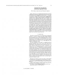
Synchronous Sequential Computation with Molecular Reactions ∗

Hua Jiang, Marc Riedel, Keshab Parhi Department of Electrical and Computer Engineering University of Minnesota 200 Union St. S.E. Minneapolis, MN 55455

{hua, mriedel, parhi}@umn.edu  ABSTRACT Just as electronic systems implement computation in terms of voltage (energy per unit charge), molecular systems compute in terms of chemical concentrations (molecules per unit volume). Prior work has established mechanisms for implementing logical and arithmetic functions including addition, multiplication, exponentiation, and logarithms with molecular reactions. In this paper, we present a general methodology for implementing synchronous sequential computation. We generate a four-phase clock signal through robust, sustained chemical oscillations. We implement memory elements by transferring concentrations between molecular types in alternating phases of the clock. We illustrate our design methodology with examples: a binary counter as well as a four-point, two-parallel FFT. We validate our designs through ODE simulations of mass-action chemical kinetics. We are exploring DNA-based computation via strand displacement as a possible experimental chassis.

Categories and Subject Descriptors I.6.5 [Simulation and Modeling]: Model Development—Modeling Methodologies

General Terms Design

Keywords Molecular Computation, Synthetic Biology, Computational Biology, Digital Design, Synchronous Logic, Sequential Logic

1.

INTRODUCTION

There has been a groundswell of interest in molecular computation in recent years [12, 14, 17, 23]. Broadly, the field strives for molecular implementations of computational processes – that is to say processes that transform input concentrations of chemical types into output concentrations of chemical types. Some of the ∗

This work is supported by an NSF EAGER Grant, #CCF0946601.

early work in the field discussed molecular solutions to challenging combinatorial problems such as the Hamiltonian Path Problem and Boolean Satisfiability [1]. In spite of the claims of “massive parallelism” – 100 Teraflop performance in a test tube! – such applications were never compelling. Chemical systems are inherently slow and messy, taking minutes or even hours to finish, and producing fragmented results. Such systems will never be competitive with conventional silicon computers for tasks such as number crunching. And yet the broad impetus of the field is not computation per se. Rather it is the design of “embedded controllers” – chemical reactions, engineered into biological systems such as viruses and bacteria, to perform useful molecular computation in situ where it is needed. For example, consider a system for chemotherapy drug delivery with engineered bacteria. The goal is to get bacteria to invade tumors and selectively produce a drug to kill the cancerous cells. Embedded control of the bacteria is needed to decide where and how much of the drug they should deliver. The computation could be as simple as: “If chemical type X is present, produce chemical type Y ” where X is a protein marker of cancer and Y is the chemo drug. Or it could be more complicated: produce Z if X is present and Y is not present or vice-versa (i.e, an exclusive-or function). Or it could be time-varying computation: produce Z if the rate of change of X is within certain bounds (i.e., band-pass filtering). Exciting recent work along these lines includes [2] and [18]. There have been deliberate attempts to bring concepts from digital circuit design into the field [3, 4, 5, 20, 19, 22, 21]. Prior work has established mechanisms for implementing specific computational constructs: logical operations such as copying, comparing and incrementing/decrementing [15]; programming constructs such as “for” and “while” loops [16]; arithmetic operations such as multiplication, exponentiation and logarithms [15, 16]; and signal processing operations such as filtering [9, 13]. Building on this prior work, we present a general methodology for implementing synchronous sequential computation.

1.1

Computational Model

A molecular system consists of a set of chemical reactions, each specifying a rule for how types of molecules combine. For instance, k

A + B −→ 2C

specifies that one molecule of A combines with one molecule of B to produce two molecules of C. The value k is called the kinetic constant. We model the molecular dynamics in terms of mass-action kinetics [7, 8]: reaction rates are proportional to (1) the quantities of the participating molecular types; and (2) the kinetic constants. Accordingly, for the reaction above, the rate of

Permission to make digital or hard copies of all or part of this work for personal or classroom use is granted without fee provided that copies are not made or distributed for profit or commercial advantage and that copies bear this notice and the full citation on the first page. To copy otherwise, to republish, to post on servers or to redistribute to lists, requires prior specific permission and/or a fee. DAC'11, June 5-10, 2011, San Diego, California, USA Copyright © 2011 ACM 978-1-4503-0636-2/11/06...$10.00

836 Permission to make digital or hard copies of all or part of this work for personal or classroom use is granted without fee provided that copies are

(1)

45.4

change in the concentrations of A, B and C is −

d[A] d[B] d[C] =− =2 = k[A][B], dt dt dt

(2)

Molecular Concentrations (Input )

(here [·] denotes concentration). Most prior schemes for molecular computation depend on specific values of the kinetic constants: the formulas that they compute include the k’s. This limits the applicability since the kinetic constants are not constant at all; they depend on factors such as cell volume and temperature. So the results of the computation are not robust. We aim for robust constructs: in our methodology we use only coarse rate categories (“fast” and “slow”). Given such categories, the computation is exact and independent of the specific reaction rates. In particular, it does not matter how fast any “fast” reaction is relative to another, or how slow any “slow” reaction is relative to another – only that “fast” reactions are fast relative to “slow” reactions.

1.2

Organization

SYNCHRONOUS SEQUENTIAL COMPUTATION

The general structure of our design is illustrated in Figure 1. As in an electronic system, our molecular system has separate constructs to implement computation and memory. A clock signal synchronizes transfers between computation and memory. For the computational reactions, we refer the reader to prior work [9, 15, 16]. Operations such as addition and scalar multiplication are straightforward. Operations such as multiplication, exponentiation, and logarithms are trickier. These can be implemented with reactions that implement iterative constructs analogous to “for” and “while” loops. (They do so robustly and exactly, without any specific dependence on the rates.) The main contributions of this paper include a new method for clock signal generation and for implementing memory.

2.1

Reactions that Preserve Concentrations (Memory)

Chemical Oscillation (Clock)

Figure 1: Block diagram of a synchronous sequential system.

The rest of the paper is organized as follows. In Section 2, we present a design methodology for synchronous sequential computation, based on clocking with chemical oscillations. We implement memory elements – flip-flops – by transferring concentrations between molecular types in alternating phases of the clock. In Sections 3 and 4, we present two detailed design examples: a three-bit binary counter and a four-point, two-parallel FFT. In Section 5, we present simulations. Finally, in Section 6, we conclude the paper with a discussion of possible experimental applications and future directions.

2.

Molecular Concentrations (Output )

Reactions that Transform Concentrations (Computation)

Clock Generation

In electronic circuits, a clock signal is generated by an oscillatory circuit that produces periodic voltage pulses. For a molecular clock, we choose reactions that produce sustained oscillations in the chemical concentrations. With such oscillations, a low concentration corresponds to logical value of zero; a high concentration corresponds to a logical value of one. Techniques for generating chemical oscillations are well established in the literature. Classic examples include the Lotka-Volterra, the “Brusselator” and the Arsenite-Iodate-Chlorite systems [6, 10]. Unfortunately, none of these schemes are quite suitable for synchronous sequential computation: we require that the clock signal be perfectly symmetrical, with abrupt transitions between the phases. Here we present a new design for a four-phase chemical oscillator. The clock phases are represented by molecular types R(ed), G(reen), B(lue), and Y (ellow). First consider the reactions:

837

∅ ∅ ∅ ∅

slow

−→ slow −→ slow −→ slow −→

r g b y

(3)

and

R+r G+g B+b Y +y

fast

−→ fast −→ fast −→ fast −→

R G B Y.

(4)

In Reactions 3, the molecular types r, g, b, and y are generated slowly and constantly. Here the symbol ∅ indicates “no reactants” meaning the products are generated from a large or replenishable source. In Reactions 4, the types R, G, B, and Y quickly consume the types r, g, b, and y, respectively. Call R, G, B, and Y the phase signals and r, g, b, and y the absence indicators. The latter are only present in the absence of the former. The reactions R+y G+r B+g Y +b

slow

−→ slow −→ slow −→ slow −→

G B Y R

(5)

transfer one phase signal to another, in the absence of the previous one. The essential aspect is that, within the RGBY sequence, the full quantity of the preceding type is transfered to the current type before the transfer to the succeeding type begins. To achieve sustained oscillation, we introduce positive feedback. This is provided by the reactions slow

2G R + IG

−* )−

IG

−→

3G

fast fast

slow

2B G + IB

−* )−

IB

−→

3B

fast fast

slow

−* )−

IY

B + IY

−→

3Y

2R

−* )−

IR

−→

3R.

2Y

fast fast

slow

Y + IR

fast fast

(6)

45.4

100

D’1,…,n (First Stage)

R B

90 80

Unitless Concentration

70

Computations

Blue Phase

Red Phase

60 50

D1,…,n (Second Stage)

40 30 20

Figure 3: The two-phase memory transfer scheme. 10 0 0

100

200

300

400 500 Unitless Time

600

700

800

The red phase reactions are

Figure 2: ODE simulation of the chemical kinetics of the proposed clock.

Consider the first two reactions. Two molecules of G combine with one molecule of R to produce three molecules of G. The first step in this process is reversible: two molecules of G can combine, but in the absence of any molecules of R, the combined form will dissociate back into G. So, in the absence of R, the quantity of G will not change much. In the presence of R, the sequence of reactions will proceed, producing one molecule of G for each molecule of R slow that is consumed. Due to the first reaction 2G −→ IG , the transfer will occur at a rate that is super-linear in the quantity of G; this speeds up the transfer and so provides positive feedback.1 Suppose that the initial quantity of R is set to some non-zero amount and the initial quantity of the other types is set to zero. We will get an oscillation among the quantities of R, G, B, and Y . We choose two nonadjacent phases, R and B, as the clock phases. Our scheme for chemical oscillation works remarkably well. Figure 2 shows the concentrations of R and B as a function of time, obtained through ordinary differential equation (ODE) simulations of the Reactions 3, 4, 5 and 6. We note that the R (red) and B (blue) phases are non-overlapping.

2.2

Memory

To implement sequential computation, we must store and transfer signals across clock cycles. In electronic systems, storage is typically implemented with flip-flips. In our molecular system, we implement storage and transfer using a two-phase protocol, synchronized on phases of our clock. Every memory unit Si is assigned two molecular types Di0 and Di . Here Di0 is the first stage and Di the second. The blue phase reactions are: B + Di Computations

fast

−→ Computations + B fast −→ Dj0 .

(7)

Every unit Si releases the signal it stores in its second stage Di . The released signal is operated on by reactions in computational modules. These generate results and push them into the first stages of succeeding memory units. Note that Dj0 molecules will be the first stage of any succeeding memory unit Sj along the signal path from Si . 1 A rigorous discussion of chemical kinetics is beyond the scope of this paper. Interested readers can consult [6].

838

R + Dj0

fast

−→ Dk + R.

(8)

Every unit Sj transfers the signal it stores in Dj0 to Dk , preparing for the next cycle. For the equivalent of delay (D) flip-flops in digital logic, j = k. For other types of memory units, j and k can be different. For example, for a toggle (T) flip-flop, Sk is the complementary bit of Sj : Dj0 −→ Dk and Dk0 −→ Dj toggle the pair of bits in each clock cycle. The transfer diagram for our memory design is shown in Figure 3.

3.

A BINARY COUNTER

As our first design example, we present a three-bit binary counter. (It can readily be generalized to an arbitrary number of bits.). The counter consists of three identical stages, each of which processes a single bit. The block diagram of a stage is shown in Figure 4a. In the nth stage, there are two memory units T1n and T0n that form a T flip-flop. The presence of molecules of T1n indicates that this bit is logical one; the presence of molecules of T0n indicates that this bit is logical zero. If we provide a non-zero initial concentration to one of the two types, then either T0n or T1n will always be present. Applying the memory implementation discussed in Section 2.2, we have types T10n and T00n as the first stages of the memory units. The red phase reactions are R + T10n R + T00n

fast

−→ T0n + R fast −→ T1n + R.

(9)

These toggle each bit. The blue phase reactions are I n−1 + T0n I n−1 + T1n

fast

−→ T00n fast −→ T10n + I n .

(10)

These simply feed the output of each T flip-flop back to its input. Note that the T flip-flops transfer molecules only when there are molecules of I n−1 injected from the previous stage. If the bit is logical one, i.e., T1n is present, then molecules of I n are injected into the next stage. Figure 4b illustrate three connected stages. Reaction B + Inj

fast

−→ I 0 + B 0

(11)

transfers the external injection Inj to I in the blue phase. Since this reaction is the very first of all computational reactions, all injection signals I n are generated in the blue phase. Accordingly, B is not required in Reaction 10, so long as I n is among the reactants.

45.4

S0

S’1

S’0

S1

T flip-flop T’0n

T0n

T’1n

T1n

In CLK

In-1

T1n

Figure 6: Generating the selection signals.

Unit for nth bit

In this system, signals are complex numbers. Both the real and the imaginary parts can be negative numbers. To represent the signals, each number X is assigned four molecular types Xp , Xn , Xp∗ , and Xn∗ . The first two are assigned to the real parts: Xp represents the positive component and Xn the negative component. The last two are assigned to the imaginary parts: Xp∗ represents the positive component and Xn∗ the negative component. Therefore, X = [Xp ] − [Xn ] + j([Xp∗ ] − [Xn∗ ]). Adders are implemented by assigning input edges and output edges to the same molecular type [9]. Note that there are two negative input edges in the lower two adders. Signals from the negative input edge will be transferred to the opposite component. For example, at the n + 1st clock cycle, M1 is transferred to O1 and O2 as

CLK In-1 (a) Block diagram of one stage of the counter. T1 2

T1 1

INJ

I0

T1 1

I1

I1

T1 2

T1 3

I2

I2

T1 3

I3

S10 + M1,p S10 + M1,n ∗ S10 + M1,p ∗ S10 + M1,n

CLK

(b) Connecting the stages. Figure 4: The binary counter.

4.

We present a second design example, a four-point two-parallel fast Fourier transform (FFT). The FFT operation is canonical in signal processing. Parallel pipelined architectures can be used for high throughput [11]. A block diagram is shown in Figure 5. Assume that the system starts at clock cycle 1. The first two inputs are sampled in cycle 1; the last two inputs are sampled in cycle 2. The system generates the first and third outputs in cycle 3; it generates the other two outputs in cycle 4. There are four switches in this design. Each selects one of the two incoming signals alternatively in different cycles. To achieve this switching functionality in our molecular design, we use two alternating selection signals. We generate these with a pair of Dflip-flops, as shown in Figure 6. If there is a non-zero initial concentration of S10 , then S00 and S10 will be “turned on” once every two cycles, in alternating fashion, starting with S10 . We implement this computation with the following reactions: fast

−→ fast −→ fast −→ fast −→

S0 + R S1 + R S00 + B S10 + B

O1,p + O2,n + S10 O1,n + O2,p + S10 ∗ O1,p + O2,n + S10 ∗ O1,n + O2,p + S10

(13)

or simply

A TWO-PARALLEL FFT DESIGN

R + S00 R + S10 B + S1 B + S0

fast

−→ fast −→ fast −→ fast −→

S10 + M1

fast

−→ O1 + O2− + S10 .

(14)

Also, for each number X, the reactions Xp + Xn Xp∗ + Xn∗

fast

−→ ∅ fast −→ ∅

(15)

are required. They cancel out equal concentrations of positive and negative components by transferring them to an external sink. There is a −j multiplication in the system. It is implemented by S10 + M2,p S10 + M2,n ∗ S10 + M2,p 0 ∗ S1 + M2,n

(12)

fast

−→ fast −→ fast −→ fast −→

0∗ D4,n + S10 0∗ D4,p + S10 0 D4,n + S10 0 D4,p + S10

(16)

or simply

The transfer reactions enabled by S10 or S00 implement the switches. Note that it is S10 and S00 , not S1 and S0 , that enable the switches, because they are generated in the blue phase.

839

S10 + M2

fast

−→ D40−∗ + S10

(17)

which transfers real/imaginary parts to imaginary/real parts with opposite polarity.

45.4

I1

M1

2n+1 2n

I2

-j 2n+1

D4

2n+1

M2

2n

O1

D3 2n+1

_

D2

O1

2n

D1

_ 2n

O2

O2

2n+1

2n Figure 5: Block diagram of a 4-point pipelined FFT design.

Based on the computational operations discussed above, we have the blue phase reactions fast

−→ fast −→ fast −→ fast −→ fast −→ fast −→ fast −→ fast −→ fast −→ fast −→ fast −→ fast −→ fast −→

D10 + S10 M1 + M2− + S00 D20 + B D10 + S00 M1 + M2− + S10 M1 + M2 + B D40−∗ + S10 D40 + S00 D30 + S00 O1 + O2− + S10 O1 + O2 + B O1 + O2− + S00 D30 + S10 .

10 9 8

(18)

7 Unitless Concentration

I1 + S10 I1 + S00 I2 + B D2 + S00 D2 + S10 D1 + B M2 + S10 M2 + S00 M1 + S00 M1 + S10 D3 + B D4 + S00 D4 + S10

set the initial concentrations of all the other molecular types to 0. We set the concentration of type Inj to 10 at time points 50, 500, 1000, 1500, 2000, 2500, and 3000. We set kfast to 100; and kslow to 1. The results of a MATLAB ODE simulation are shown in Figure 7. We see that the bit signals T10 , T11 , and T12 toggle at

6 5 4 3

D01

2

D11 D21

1

Note that S00 and S10 are generated in the blue phase. It is not necessary to list B if a reaction is enabled by S00 or S10 . The red phase reactions are R + D10 R + D20 R + D30 R + D40

fast

−→ fast −→ fast −→ fast −→

D1 + R D2 + R D3 + R D4 + R.

(19)

So the full design of the four-point, two-parallel FFT consists of Reactions 12, 18 and 19, together with the positive/negative canceling reactions as well as the clock generation reactions.

5.

SIMULATIONS

We present simulation results for the binary counter and for the FFT. For each design, we list our choice of kinetic constants corresponding to “slow” and “‘fast” as well as the initial concentrations of the molecular types. We assume that an external source sets the concentrations of the input types to new values at specific intervals. We setup ordinary differential equations corresponding to the mass-action kinetics of the reactions and solve these numerically with MATLAB.

5.1 5.1.1

Transient Response Counter

For the three-bit counter, we set the initial concentrations of T00 , T01 , and T02 to 10 (corresponding to bits “000”) and R to 100. We

840

0 0

500

1000

1500 2000 Unitless Time

2500

3000

3500

Figure 7: Transient simulation result of the counter. the correct time points. The system counts the number of injection events from “000” to “111” correctly. One observation from Figure 7 is that the concentrations of T10 , 1 T1 , and T12 when the corresponding bit is “1” degrade slowly over time. This is because of slightly overlapped clock phases. There is always a slight leakage in the amount of R in the blue phase and a slight leakage in the amount of B in the red phase. This error accumulates over time, due to the feedback loop in each stage of the counter. To mitigate against this, we could select a higher ratio fast . of λ = kkslow

5.1.2

FFT

For our FFT design, we the set initial concentration of S00 to 50 and that of R to 100. Recall that S00 is transferred to S0 in the first red phase and S0 is transferred to S10 in first blue phase. So the computation begins with S10 . We set the initial concentrations of all the other types to 0. We inject I1 and I2 in the red phase. The output types O1 and O2 are produced in clock cycle 3, in a blue phase. We clear them out in following red phase. We set kfast to 100; and kslow to 1. The results of a MATLAB ODE simulation are shown in Figure 8. The inputs are a sequence of real numbers {10, 15, 10 ,0}. The outputs are {35, -15j, 5, 15j}, as shown in the figure. Since there is no feedback in the FFT architecture, no error due to the leakage of R and B accumulates.

45.4

independent design. DNA assembly can be considered the “backend” – analogous to technology mapping to a specific library.

120 R B S’

100

0

7.[1] L.REFERENCES Adleman. Molecular computation of solutions to combinatorial

S’

1

O1,p

80

O2,p O*1,n

60

O*2,p

40

20

0

0

100

200

300

400

500

600

700

800

Figure 8: Transient simulation of the FFT design. Table 1: Relative error in simulations.

λ 10 100 1000

5.2

Counter (Average error per cycle per bit) 0.9871% 0.2078% 0.0169%

FFT 28.107% 3.5428% 0.2691%

Error Analysis

We analyze computational errors of the counter and the FFT design in terms of the fast-to-slow ratio λ. For the counter, the error is defined as the differences of concentrations from a perfect “0” or a perfect “1”. We consider the average error accumulated in one clock cycle for one bit. For the FFT design, we consider the relative error of the simulated outputs compared to theoretical outputs. These errors are listed in Table 1. As expected, we see that the error decreases as λ increases: with a higher fast-to-slow ratio, fewer reactions misfire – that is, fire in the wrong clock phase.

6.

REMARKS

This paper presents the first robust, rate-independent methodology for synchronous computation. Here “rate-independent” refers to the fact that, within a broad range of values for the kinetic constants, the computation is exact and independent of the specific rates. The results in this paper are complementary to prior results on self-timed methodologies for molecular computation [9]. Those had a distinct asynchronous flavor. As in electronic circuit design, there are advantages and disadvantages to asynchronous and synchronous design styles for molecular computing. On the one hand, a synchronous style leads to simpler designs with fewer reactions. On the other hand, errors can accumulate across clock cycles. We are exploring the mechanism of DNA strand-displacement as an experimental chassis [17]. DNA strand-displacement reactions can emulate chemical reactions with nearly any rate structure. Reaction rates are controlled by designing sequences with different binding strengths. The binding strengths are controlled by the length and sequence composition of “toehold” sequences. With the right choice of toehold sequences, reaction rates differing by as much as 106 can be achieved. Our contribution can be positioned as the “front-end” of the design flow – analogous to technology-

841

problems. Science, 266(11):1021–1024, 1994. [2] J. C. Anderson, E. J. Clarke, A. P. Arkin, and C. A. Voigt. Environmentally controlled invasion of cancer cells by engineered bacteria. Journal of Molecular Biology, 355(4):619–627, 2006. [3] J. C. Anderson, C. A. Voigt, and A. P. Arkin. A genetic AND gate based on translation control. Molecular Systems Biology, 3(133), 2007. [4] A. Arkin and J. Ross. Computational functions in biochemical reaction networks. Biophysical Journal, 67(2):560 – 578, 1994. [5] Y. Benenson, B. Gil, U. Ben-Dor, R. Adar, and E. Shapiro. An autonomous molecular computer for logical control of gene expression. Nature, 429(6990):423–429, 2004. [6] I. R. Epstein and J. A. Pojman. An Introduction to Nonlinear Chemical Dynamics: Oscillations, Waves, Patterns, and Chaos. Oxford Univ Press, 1998. [7] P. Érdi and J. Tóth. Mathematical Models of Chemical Reactions: Theory and Applications of Deterministic and Stochastic Models. Manchester University Press, 1989. [8] F. Horn and R. Jackson. General mass action kinetics. Archive for Rational Mechanics and Analysis, 47:81–116, 1972. [9] H. Jiang, A. P. Kharam, M. D. Riedel, and K. K. Parhi. A synthesis flow for digital signal processing with biomolecular reactions. In IEEE International Conference on Computer-Aided Design, pages 417–424, 2010. [10] P. D. Kepper, I. R. Epstein, and K. Kustin. A systematically designed homogeneous oscillating reaction: the arsenite-iodate-chlorite system. Journal of the American Chemical Society, 103(8):2133–2134, 2008. [11] K. K. Parhi. VLSI Digital Signal Processing Systems. John Wiley & Sons, 1999. [12] L. Qian, D. Soloveichik, and E. Winfree. Efficient turing-universal computation with DNA polymers. In International Conference on DNA Computing and Molecular Programming, 2010. [13] M. Samoilov, A. Arkin, and J. Ross. Signal processing by simple chemical systems. Journal of Physical Chemistry A, 106(43):10205–10221, 2002. [14] G. Seelig, D. Soloveichik, D. Y. Zhang, and E. Winfree. Enzyme-free nucleic acid logic circuits. In Science, volume 314, pages 1585–1588, 2006. [15] P. Senum and M. D. Riedel. Rate-independent biochemical computational modules. In Proceedings of the Pacific Symposium on Biocomputing, 2011. [16] A. Shea, B. Fett, M. D. Riedel, and K. Parhi. Writing and compiling code into biochemistry. In Proceedings of the Pacific Symposium on Biocomputing, pages 456–464, 2010. [17] D. Soloveichik, G. Seelig, and E. Winfree. DNA as a universal substrate for chemical kinetics. Proceedings of the National Academy of Sciences, 107(12):5393–5398, 2010. [18] S. Venkataramana, R. M. Dirks, C. T. Ueda, and N. A. Pierce. Selective cell death mediated by small conditional RNAs. Proceedings of the National Academy of Sciences, 2010 (in press). [19] R. Weiss. Cellular Computation and Communications using Engineering Genetic Regulatory Networks. PhD thesis, MIT, 2003. [20] R. Weiss, G. E. Homsy, and T. F. Knight. Toward in vivo digital circuits. In DIMACS Workshop on Evolution as Computation, pages 1–18, 1999. [21] M. N. Win, J. Liang, and C. D. Smolke. Frameworks for programming biological function through RNA parts and devices. Chemistry & Biology, 16:298–310, 2009. [22] M. N. Win and C. D. Smolke. A modular and extensible RNA-based gene-regulatory platform for engineering cellular function. Proceedings of the National Academy of Sciences, 104(36):14283, 2007. [23] B. Yurke, A. J. Turberfield, A. P. Mills, Jr, F. C. Simmel, and J. Neumann. A DNA-fuelled molecular machine made of DNA. Nature, 406:605–608, 2000.