remote sensing Article
Synergistic Use of LiDAR and APEX Hyperspectral Data for High-Resolution Urban Land Cover Mapping Frederik Priem * and Frank Canters Cartography and GIS Research Group, Vrije Universiteit Brussel, Brussel 1050, Belgium;
[email protected] * Correspondence:
[email protected]; Tel.: +32-2-629-3384 Academic Editors: Bailang Yu, Soe W. Myint, Clement Atzberger and Prasad S. Thenkabail Received: 7 June 2016; Accepted: 8 September 2016; Published: 22 September 2016
Abstract: Land cover mapping of the urban environment by means of remote sensing remains a distinct challenge due to the strong spectral heterogeneity and geometric complexity of urban scenes. Airborne imaging spectroscopy and laser altimetry have each made remarkable contributions to urban mapping but synergistic use of these relatively recent data sources in an urban context is still largely underexplored. In this study a synergistic workflow is presented to cope with the strong diversity of materials in urban areas, as well as with the presence of shadow. A high-resolution APEX hyperspectral image and a discrete waveform LiDAR dataset covering the Eastern part of Brussels were made available for this research. Firstly, a novel shadow detection method based on LiDAR intensity-APEX brightness thresholding is proposed and compared to commonly used approaches for shadow detection. A combination of intensity-brightness thresholding with DSM model-based shadow detection is shown to be an efficient approach for shadow mask delineation. To deal with spectral similarity of different types of urban materials and spectral distortion induced by shadow cover, supervised classification of shaded and sunlit areas is combined with iterative LiDAR post-classification correction. Results indicate that height, slope and roughness features contribute to improved classification accuracies in descending order of importance. Results of this study illustrate the potential of synergistic application of hyperspectral imagery and LiDAR for urban land cover mapping. Keywords: urban; land cover; shadow detection; shadow compensation; support vector machines; hyperspectral remote sensing; APEX; LiDAR; post-classification
1. Introduction In light of the challenges presented by climate change and urbanization, more than ever urban areas need to be monitored in order to gain a better physical understanding of this complex and dynamic environment. Over the past decades, urban remote sensing has presented itself as a viable means to systematically acquire information on different spatial, spectral and temporal scales using a wide range of spaceborne and airborne Earth observation platforms. Remote sensing of urban scenes remains a challenging topic though due to characteristic difficulties presented by the urban environment and limitations of traditional sensors. Urban areas are composed of a complex mosaic of different materials that can usually be attributed to a combination of four material components: minerals, vegetation, oil-derived products and other artificial materials including metals [1]. Each material displays specific reflectance features in the Visible Near-Infrared (VNIR) and Short Wave Infrared (SWIR) wavelength regions so consequently cities are characterized by a very high degree of spectral heterogeneity [2,3]. Adding to the complexity is the fact that some materials that are used for different purposes (e.g., roof versus road materials) do share similar material compositions and
Remote Sens. 2016, 8, 787; doi:10.3390/rs8100787
www.mdpi.com/journal/remotesensing
Remote Sens. 2016, 8, 787
2 of 22
thus also show similar spectral behavior [4]. Variations in composition within a material type, material weathering and material condition can furthermore induce a significant degree of spectral intra-class confusion [5–8]. Another concern of urban remote sensing is the complex geometry of the urban environment. Most observed urban objects tend to have rather small spatial dimensions compared to objects encountered in natural environments and these objects are often arranged in complex site-specific geometries [1,4]. The characteristic geometric assembly and the differences in surface roughness of urban areas result in substantial impact of direction-dependent reflectance properties and in the presence of shade. Both these phenomena lead to a substantial increase in heterogeneity in the measured spectral response of urban materials [8]. The complexity of urban scenes has led to an increased demand for more advanced, high resolution remote sensing solutions. Especially in the past decade there has been a steady growth in the development and availability of new sensors able to better cope with the challenges outlined above. Two technologies that have made remarkable contributions are hyperspectral remote sensing, also referred to as imaging spectroscopy, and Light Detection And Ranging (LiDAR) [9–11]. As opposed to broadband multispectral sensors, hyperspectral sensors tend to extensively cover both the VNIR and SWIR regions with a high number (ranging from tens to hundreds) of narrowly defined spectral bands, allowing them to capture even subtle spectral features, strongly improving the ability to discriminate different materials and in some cases even material conditions [10]. LiDAR technology can be described as a laser profiling and scanning system emitting monochromatic NIR pulses that produce very dense point clouds in which each point is accurately positioned in 3D using direct geo-referencing. As such, LiDAR is a powerful tool for altimetric modelling of nearly any terrain [9]. The advent of LiDAR marked a major step forward in urban remote sensing since it allowed to move beyond the limits dictated by multi- and hyperspectral imagery by adding new components to the equation such as height, intensity and multiple return/texture features [9,12–15]. Despite the merits that hyperspectral and LiDAR data possess on their own, it is mainly through synergistic use of both these technologies that urban mapping has managed to produce some of its most interesting and promising results in recent years [16–20]. Data fusion of imaging spectroscopy and laser altimetry or hyperspectral-LiDAR synergy is a young but dynamic research field that has only started to develop fully in the last decade. Approaches for synergy can be differentiated based on how the LiDAR data are integrated in the land-cover mapping workflow: through vector stacking (feature selection or pre-processing), re-classification or in a post-classification phase [21]. Vector stacking should be understood as a process of combining raw spectral, textural or object-based features derived from a hyperspectral image and a LiDAR point cloud before being used as input for a classifier [22]. Given the completely different nature of hyperspectral and LiDAR data, machine learning classifiers are preferred in this approach, since these classifiers are non-parametric and do not make assumptions regarding the distribution of the input variables [23]. Re-classification involves a two-step mapping process where the first step consists of a classification based on hyperspectral data, which is followed by a second classification using the output of the spectral classifier and LiDAR derived features as its input. More than just improving the accuracy of the spectral classification, adding height (derived) information can improve thematic detail in land cover mapping [18]. Finally, post-classification involves the improvement of classification output using external data (in this case LiDAR) in combination with a specific ruleset. Rulesets for post-classification can be constructed manually or semi-automatically using discrete thresholds, soft classification output, object-based and/or statistical information in order to perform correction [24]. A number of examples can be found in the literature where multiple approaches for hyperspectral-LiDAR synergy are combined within one workflow [17,18]. Regardless of the approach, LiDAR height information and derivatives naturally complement hyperspectral data because they may allow discriminating between geometrically dissimilar but spectrally similar material classes. Use of LiDAR data in combination with hyperspectral data may also prove useful for dealing with the omnipresence of shadow in urban areas. Shadow is the result of a complete or partial
Remote Sens. 2016, 8, 787
3 of 22
blocking of direct irradiance. It is particularly problematic for analysis of imagery covering cities with a strong degree of high-rise development or strong topographic features. Likewise, imagery acquired before or after solar noon, outside of the summer season, during cloudy weather conditions or in temperate to arctic climate zones may be severely tainted by shadow [25,26]. Whereas for sunlit surfaces direct irradiance will be the main contributing factor to the total radiance budget, for shaded areas the relative contributions of environmental and atmospheric radiance will be far greater while direct irradiance may even be reduced to zero [27]. Because shadow distorts the spectral signature of materials, accurate mapping of urban areas requires dedicated approaches to deal with shadow. A distinction can be made between shadow detection and shadow compensation techniques. Shadow detection answers the question where and to what extent shadow occurs in an image [28]. Shadow compensation on the other hand encompasses methods that can be used to reduce or avoid the impact of shadow cover on mapping [29]. A considerable number of shadow detection and compensation techniques have been developed for remote sensing but most focus on high resolution multispectral data. Only more recently have techniques been proposed that attempt to benefit from LiDAR and hyperspectral imagery. Model-based or geometric shadow detection approaches utilize a-priori information, in most cases Digital Surface Models (DSM) and solar illumination angles at the time of image acquisition, to perform line-of-sight analysis or ray tracing [30–33]. These geometric approaches have the advantage of avoiding errors in shadow detection induced by spectral confusion but their output will be directly dependent on the quality of the DSM and its co-registration with the image data. Color Invariant approaches, on the other hand, select certain image bands, spectral indices or color space components that are (near) insensitive to lighting conditions and compare those with light dependent features [34]. Machine learning shadow detection relies on the unique spectral characteristics of shaded materials to detect shadow induced spectral features. Support Vector Machines (SVM) are currently prevalent classification algorithms used for this purpose [35]. The main drawback of the machine learning approach, however, is the need to produce a dedicated training dataset of shaded areas, which can be very difficult and labor intensive. Machine learning shadow detection methods will be inclined to produce more satisfying results when used with high resolution spectral information, but will in any case still be prone to spectral confusion [28,29]. Shadow compensation includes a wide range of methods. A differentiation can be made between pre-processing, classification and post-processing techniques. Illumination effects in hyperspectral imagery can be suppressed in pre-processing by converting radiance or reflectance information to spectral angles and linearly correcting them based on shadow/non-shadow statistics [36]. A more intricate method to compensate for the effect of shadow in hyperspectral urban imagery using LiDAR information has been proposed in [37]. Here, a DSM and other LiDAR derived features such as sky view factor are used to model different irradiance components which are in turn entered in a non-linear spectral correction model. Direct classification or classification of shaded areas using shaded material training data is a shadow compensation technique that has been applied with relative success for classifying multispectral imagery [38] but remains remarkably unexplored for hyperspectral data. This approach relies on the idea that radiances received from shaded areas are still material dependent and assumes that a significant amount of class related spectral information is still present in shadow [28]. Shadow compensation can also be achieved in a post-classification phase by training a machine learning classifier with a separate shadow class and then running a second, dedicated classifier to assign shadow pixels identified in the first step to meaningful non-shadow classes [24]. Few studies so far have combined airborne hyperspectral and LiDAR data for accurate urban land cover mapping on a high level of thematic detail, exploiting LiDAR for shadow detection as well as improvement of land-cover classification output. Dealing with shadow remains a topic that has been mainly explored for urban mapping with multispectral high-resolution imagery. The general objective of this paper is to investigate the potential of hyperspectral-LiDAR synergy for urban land cover mapping when faced with strong spectral heterogeneity of materials, between-class spectral confusion and shadow cover. Three specific research objectives are envisioned: (1) defining a novel
Remote Sens. 2016, 8, 787
4 of 22
approach for shadow detection in urban scenes by combining hyperspectral imagery with LiDAR features; (2) assessing the performance of hyperspectral SVM classification in shadow and non-shadow areas, using both sunlit and shaded training data for a large variety of urban materials; (3) assessing the added value of different height-derived LiDAR features for post-classification improvement of hyperspectral classification output. The two primary data sources used in this research are an APEX airborne hyperspectral image and a discrete waveform LiDAR dataset, both covering a NW–SE urban transect in the eastern part of the Brussels Capital Region (BCR). In the first part of the paper, a novel intensity-brightness thresholding technique for shadow detection is proposed. Next, a detailed mapping of urban land cover in both shaded and non-shaded areas is performed, using Support Vector Classification (SVC). SVC has been selected based on its flexibility, robustness, relative ease of use, performance and its soft class probability output. Finally, an iterative post-classification correction algorithm using SVC class membership probabilities and LiDAR features is proposed and tested on the APEX hyperspectral classification result. This study illustrates the strengths of combining airborne imaging spectroscopy and laser altimetry for urban material mapping as well as the potential of APEX hyperspectral data, when used in combination with high-resolution LiDAR data. 2. Materials and Methods 2.1. Data and Study Area 2.1.1. APEX Hyperspectral Imagery and Image Preprocessing The Airborne Prism Experiment or APEX sensor is a dispersive pushbroom imaging spectrometer designed for airborne applications as well as simulation and calibration of (future) spaceborne missions. The sensor has a spectral coverage of 372–2540 nm but the number and widths of the spectral bands can be configured for the purpose of the application [39,40]. An APEX image was acquired on 8 July 2013 around 11 h local time covering the eastern part of the Brussels Capital Region and most of the Sonian forest (Figure 1). The East of the BCR is characterized by a strongly heterogeneous urban fabric composed of residential, commercial service-oriented and mixed function areas with differing densities, as well as leisure infrastructure, parks and other green spaces. Four NW-SE oriented flight lines were needed to cover the study area, each recorded at an altitude of approximately 3650 m a.s.l. The instrument was configured to perform measurements over 288 spectral bands but bands 147–160 and 198–219 were removed from further analyses due to atmospheric absorption effects, leaving 252 bands. The initial level 1C product was geometrically corrected using direct georeferencing and atmospherically corrected using the MODTRAN4 radiative transfer code to derive bottom-of atmosphere reflectance [41–44]. The final level 2B image was registered in the Belgian Lambert 72 coordinate system with dimensions encompassing 8860 rows by 3491 columns and a pixel size of 2 × 2 m2 . To ease computational burdens, use was made of the BandClust dimensionality reduction algorithm. BandClust is a recursive non-parametric semi-unsupervised band clustering algorithm that employs minima in Mutual Information plots over a range of adjacent bands to find optimal splitting points. Bands located between two splitting bands are clustered by averaging in order to acquire a reduced number of bands. For more information on the BandClust algorithm the reader is referred to [45]. A total of 21 bands was retained after performing BandClust. Previous research with APEX on the BCR has shown that BandClust has no negative impact on classification accuracies compared to using the full hyperspectral image dataset when working with a large number of urban classes [46]. Also, in this study, comparative kappa analysis did confirm that use of BandClust did not result in lower classification accuracies compared to using all bands, but even improved image classification accuracy slightly.
Remote Sens. 2016, 8, 787 Remote Sens. 2016, 8, 787
5 of 22 5 of 22
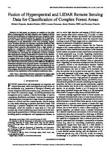
Figure Figure 1. 1. (a) (a) RGB-image RGB-image (R (R == band 36, 36, G G == band 18 and B = = band 5) of the 2013 APEX APEX image image covering covering the of the Capital RegionRegion and (b) and inset(b) mapinset for VUB Annotations the Eastern Easternpart part of Brussel the Brussel Capital mapuniversity for VUBcampus. university campus. in (b) refer to in material spectra (see below). Annotations (b) refer to material spectra (see below).
in this comparative 2.1.2.Also, LiDAR and study, Derived Features kappa analysis did confirm that use of BandClust did not result in lower classification accuracies compared to using all bands, but even improved image classification An airborne discrete waveform LiDAR dataset acquired in the winter of 2012 with an average accuracy slightly. point density of 35 points/m2 after point filtering has been used for this study (LiDAR data provided by theLiDAR Brusselsand Regional Informatics 2.1.2. Derived Features Centre). The original extent covering the whole BCR was reduced to that of the hyperspectral image and a 25 cm resolution DSM was extracted using the LAS dataset An tool airborne discrete waveform dataset acquired thebinning. winter of 2012 with average to raster provided in ArcGIS withLiDAR maximum height valuesinfor Linear void an filling was pointto density of 35 points/m² pointalthough filtering has been used fordue thistostudy (LiDAR provided used interpolate caveats inafter the DSM these were rare the very highdata LiDAR point by the Brussels Regional Informatics Centre). The extent covering the resampled whole BCRtowas density. Subsequently, this DSM was co-registered withoriginal the hyperspectral image and the reduced to that of the hyperspectral image and a 25 cm resolution DSM was extracted using theDSM LAS APEX 2 m resolution. Performing this two-step procedure proved to avoid oversensitivity of the dataset to raster tool provided ArcGISin with height values binning.and Linear voidcables). filling to narrow tall or linear objectsinpresent the maximum urban environment (e.g.,for antennae power was used to interpolate caveats in the DSM although these were rare due to the very high LiDAR A normalized DSM or nDSM at 2 m resolution describing the height of pixels above ground level, was point density. Subsequently, this DSM Digital was co-registered with(DEM) the hyperspectral produced by subtracting a LiDAR derived Elevation Model from the DSM image (Figure and 2a). resampled to the APEX 2 m resolution. Performing this two-step procedure proved to avoid From the 25 cm DSM, a slope image was extracted which was in turn used to construct a roughness oversensitivity of theRoughness DSM to narrow tall or linear objects in the urban environment (e.g., image (Figure 2b,c). was acquired by taking thepresent standard deviation of all 25 cm slope antennae and within power acables). A normalized or nDSM atby2 taking m resolution describing the height pixels located 2 m pixel, while slopeDSM was calculated the mean value. By means ofof a pixels above ground level, was produced by subtracting a LiDAR derived Digital Elevation Model procedure similar to that for DSM extraction but with average binning, a LiDAR intensity image was (DEM) from the DSM (Figure intensity 2a). Fromrepresents the 25 cm the DSM, a slope imageofwas extracted which was in produced (Figure 2d). LiDAR peak amplitude a backscattered pulse and turn usedthis to measure constructis asubject roughness image (Figure 2b,c). was acquired by study takingis the although to a number of factors, whatRoughness is mainly important for this its standard deviation of all 25 cm slope pixels located within a 2 m pixel, while slope was calculated by correlation with inherent surface brightness and near insensitivity to surface lighting conditions. These taking thecharacteristics mean value. By of adetection procedure similar to that for further DSM extraction with average are useful formeans shadow as will be illustrated on. It hasbut to be noted that binning, a LiDAR intensity image was produced (Figure 2d). LiDAR intensity represents the peak due to sensor-to-surface angles of incidence and scattering effects of LiDAR pulses on oblique and very amplitude of a (e.g., backscattered andvalues although is subjectfor to aeach number of factors, what rough surfaces canopy), pulse intensity willthis not measure be representative material class. Since is mainlywas important thisunitless study is its correlation inherent surface brightness near intensity deliveredfor in the range of [0, 1500], with this range has been rescaled to [0, 1]and in order insensitivity to surface lighting conditions. These are useful characteristics for shadow detection as to avoid computational issues during classification and to facilitate comparison with brightness data. will be illustrated further on. It has to be noted that due to sensor-to-surface angles of incidence and scattering effects of LiDAR pulses on oblique and very rough surfaces (e.g., canopy), intensity values will not be representative for each material class. Since intensity was delivered in the unitless range of [0, 1500], this range has been rescaled to [0, 1] in order to avoid computational issues during classification and to facilitate comparison with brightness data.
Remote Sens. 2016, 8, 787 Remote Sens. 2016, 8, 787
6 of 22 6 of 22
Figure illustrated forfor thethe VUB university campus withwith (a) Figure 2. 2. LiDAR LiDARfeatures featuresused usedininthis thisresearch research illustrated VUB university campus normalized DSM; (b) slope; (c) roughness and (d) intensity (expressed in uncalibrated Digital (a) normalized DSM; (b) slope; (c) roughness and (d) intensity (expressed in uncalibrated Digital Numbers Numbers (DN)). (DN)).
2.1.3. High-Resolution Orthophotos Orthophotos and and other other Ancillary Ancillary Data Data 2.1.3. Very Very High-Resolution A A 2012 2012 winter winter acquisition acquisition RGB-NIR RGB-NIR orthophoto orthophoto with with aa resolution resolution of of 7.5 7.5 cm, cm, obtained obtained from from the the Brussels producing Brussels Regional Regional Informatics Informatics Centre, Centre, was was used used as as visual visual reference reference for for the the purpose purpose of of producing ground datasets from thethe UrbIS spatial database of ground truth truth data data over overthe thestudy studyarea. area.Ancillary Ancillaryvector vector datasets from UrbIS spatial database Brussels², water and building shapefiles, improve 2 , including of Brusselsincluding water and building shapefiles,have havebeen beenutilized utilizedininthis this study study to to improve classification results in post-processing. Google Street View proved to be invaluable in assisting classification results in post-processing. Google Street View proved to be invaluable in assisting in in discriminating differentmaterials materialsatatstreet streetlevel, level,both both and of shadow. Oblique aerial imagery discriminating different inin and outout of shadow. Oblique aerial imagery has has to complement the mentioned earlier mentioned orthophotos for discrimination material discrimination also also beenbeen used used to complement the earlier orthophotos for material (acquired (acquired at http://geoloc.irisnet.be). at http://geoloc.irisnet.be). 2.2. 2.2. Methodology Methodology 2.2.1. Classification Scheme and Sampling Strategy The complete workflow adopted in this study is depicted in Figure 3. All steps will be explained paragraphs. The The first first step step in in the the workflow workflow was was the the design design of a in further detail over the following paragraphs. hierarchical classification classification scheme scheme in in which which level level 2 or the material class level is of particular interest hierarchical For clarity’s clarity’s sake, sake, all all mention mention of of land land cover cover classes classes will will refer refer to level 2 unless explicitly (Table 1). For otherwise. AA total total of of 27 27 classes classes were were included included in in the the scheme scheme describing describing some some of of the most stated otherwise. but also some thatthat havehave onlyonly recently been been introduced in the in urban common urban urbanmaterials materials(Figure (Figure4)4) but also some recently introduced the landscape on a significant scale (e.g., reflective hydrocarbon roofing, extensive green urban landscape on a significant scalesolar (e.g.,panels, solar panels, reflective hydrocarbon roofing, extensive green roofs). Note that bright roof material is actually a conglomerate of different white PVC, EPDM and other bright hydrocarbon roofing materials as well as bright coatings applied on metal roofs.
Remote Sens. 2016, 8, 787
7 of 22
Remote Sens. 2016, 8, 787 of 22 roofs). Note that bright roof material is actually a conglomerate of different white PVC, EPDM7 and other bright hydrocarbon roofing materials as well as bright coatings applied on metal roofs. Attempts Attempts to map these asclasses separate classes were unsuccessful due to theirsimilarity spectral similarity since to map these as separate were unsuccessful due to their spectral and sinceand all these all these materials serve the same purpose of providing bright impervious roofing, the decision materials serve the same purpose of providing bright impervious roofing, the decision was madewas to made to cluster them. Reflective hydrocarbon also mainlyofconsists of EPDM PVC and EPDM based roofing cluster them. Reflective hydrocarbon also mainly consists PVC and based roofing materials materials butprevailing here the prevailing colorsand aretogray and extent to a lesser extent green and red. but here the colors are gray a lesser green and red.
Figure 3. 3. Flowchart outlining outlining the the workflow workflow implemented implemented in in this this research. research. Figure
Figure 4. Examples of different material spectra sampled from the APEX image and included in the set Figure 4. Examples different material from theNotice APEXthat image and included the of ground truth data of with (a) sunlit spectraspectra and (b)sampled shaded spectra. the materials havein been set of ground truth data annotated in Figure 1b. with (a) sunlit spectra and (b) shaded spectra. Notice that the materials have been annotated in Figure 1b.
For each class, a set of sunlit ground truth polygons with a maximum size of 12 APEX pixels was For each class, ausing set ofall sunlit ground truth polygons with Except a maximum size of 12 APEX pixels was manually digitized available data described above. for a limited number of classes, manually digitized using all available data above. Except a limited number classes, 250–300 spectra were collected per class. In described addition, shaded groundfor truth polygons wereof digitized 250–300 spectra were collected per class. In addition, shaded ground truth polygons were digitized for as many material classes as was deemed feasible. Classes with only a marginal occurrence in for as many as was deemed feasible. Classes withThe only a marginal occurrence in shadow were material excludedclasses and finally 17 out of 27 classes were covered. amount of digitized shaded shadow were excluded and finally 17 out of 27 classes were covered. The amount of digitized shaded polygons is however considerably lower than the amount of sunlit polygons (Table 1). Subsequently, polygons however thanwere the amount polygons (Table 1).sets Subsequently, the shadedisand sunlit considerably ground truth lower polygons each splitofinsunlit training and validation based on a the shaded and sunlit ground truth polygons were each split in training and validation sets based on 1/3 training and 2/3 validation stratified sampling scheme. Given that the applied SVM classifier is a 1/3 training and 2/3 validation stratified sampling scheme. Given that the applied SVM classifier is known to retain its ability to generalize even with a limited training sample size, this split ratio was known to retain its ability to generalize even with a limited training sample size, this split ratio was deemed appropriate for this study. The ground truth set of shaded polygons was already limited to deemed for this study. The ground set of shaded polygons was already limited to start withappropriate and the adopted sampling scheme thustruth ensures a representative accuracy assessment. start with and the adopted sampling scheme thus ensures a representative accuracy assessment.
Remote Sens. 2016, 8, 787
8 of 22
Table 1. Hierarchical classification scheme adopted for this study with indication of number of sunlit-shaded ground truth polygons and pixels for each level 2 material class. Level 1
Level 2
Sunlit Polygons
Sunlit Pixels
roof
1. red ceramic tile 2. dark ceramic tile 3. dark shingle 4. bitumen 5. fiber cement 6. bright roof material 7. hydrocarbon roofing 8. gray metal 9. green metal 10. paved roof 11. glass 12. gravel roofing 13. green roof 14. solar panel 15. asphalt 16. concrete 17. red concrete pavers 18. railroad track 19. cobblestone 20. bright gravel 21. red gravel 22. tartan 23. artificial turf 24. green surface 25. high vegetation 26. low vegetation 27. bare soil 28. water◦
25 35 33 29 28 27 30 15 20 28 13 30 24 28 27 29 28 29 20 19 28 17 26 25 27 27 31 n/a
247 307 280 260 306 311 308 143 216 302 153 322 258 309 313 328 312 300 229 195 309 198 307 282 312 306 342 n/a
pavement
high vegetation low vegetation bare soil water◦
◦
Shaded Polygons
Shaded Pixels
16 26 12 11 14 12
99 150 121 92 122 115
11
99
17 17 14 12 10 13 10
158 159 105 91 100 135 112
9
112
14 14
107 133
n/a
n/a
= manually classified with mask.
2.2.2. Shadow Detection A novel shadow detection method is presented here that is inspired by Invariant Color Model shadow detection. The idea of the approach proposed is to use LiDAR derived intensity as an image-external lighting invariant feature, more specifically as a proxy for inherent surface brightness of the APEX image. The first step of the procedure encompasses taking the ratio of LiDAR intensity (scaled to a [0, 1] range) over APEX image brightness. Brightness is calculated simply by taking the average reflectance for each pixel. In this ratio image, high pixel values represent areas where inherent or expected brightness is high compared to the observed brightness in the APEX image. The assumption is made that such areas are affected by cast shadow. In the second step, a manually determined threshold value is applied on the ratio image resulting in a binary shadow mask. A threshold value of 4 was found to cover almost all fully shaded areas without giving rise to overestimation. It should be noted that this shadow detection approach is not suited for identifying areas affected by partial shadow cover or self-shadow. In order to detect those brighter types of shadow, a lower threshold value would be needed but tests indicated that this results in an overestimation of shadow cover on darker sunlit areas. To allow comparison with other approaches for shadow detection, a machine learning and a geometry-based shadow mask were produced. The former was obtained by training a two class SVM classifier with shaded and sunlit training data, the latter by applying the shadow volume approach proposed by [32] on the 25 cm DSM using solar angles at the time of APEX image acquisition [31–33]. The shadow volume approach was implemented by developing a Matlab function that iteratively shifts the DSM in the horizontal direction of cast shadow dx and dy while uniformly subtracting a corresponding decrease in height dz from the DSM. This process continues until the accumulated change in height surpasses the maximal height difference in the DSM or until a predefined number of
Remote Sens. 2016, 8, 787
9 of 22
Remote Sens. 2016, 8, 787
9 of 22
iterations has been reached that reasonably allows all shadows to be fully projected. A near zenith solar solar height height will cast smaller shadows requiring fewer iterations iterations and vice versa. The resulting shadow volume volume model model can subsequently subsequently be be converted converted into into a shadow mask simply by subtracting the original DSM from it and and converting converting all all positive positive values values to to 11 (Figure (Figure 5). 5).
Figure 5. 5. Overview Overview of of the the DSM DSM model-based model-based shadow shadow detection detection approach, approach, in in this this paper paper referred referred to to as as Figure shadow volume approach. shadow volume approach.
2.2.3. Support Vector Classification 2.2.3. Support Vector Classification Support Vector Machines are a group of non-parametric statistical machine learning methods Support Vector Machines are a group of non-parametric statistical machine learning methods that that are capable of solving complex non-linear classification and regression problems. SVM has are capable of solving complex non-linear classification and regression problems. SVM has proven proven itself to be robust even when faced with low observations to dimensionality training samples itself to be robust even when faced with low observations to dimensionality training samples [47]. [47]. Not surprisingly, Support Vector Classification has witnessed a drastic growth in popularity Not surprisingly, Support Vector Classification has witnessed a drastic growth in popularity over the over the past decades in many different scientific disciplines, including remote sensing [48,49]. For past decades in many different scientific disciplines, including remote sensing [48,49]. For this study, this study, the imageSVM Classification tools provided by the EnMAP-box software were used to the imageSVM Classification tools provided by the EnMAP-box software were used to perform SVC [50]. perform SVC [50]. The SVC tools included in EnMAP-box are based on the LIBSVM algorithm. The The SVC tools included in EnMAP-box are based on the LIBSVM algorithm. The primary output is primary output is a class probability image from which a class image is derived by selecting the class a class probability image from which a class image is derived by selecting the class with the highest with the highest probability for each pixel [51]. A Support Vector Classification was performed using probability for each pixel [51]. A Support Vector Classification was performed using all sunlit and all sunlit and shaded training data. The output was subjected to a majority filter with a 3 × 3 pixel shaded training data. The output was subjected to a majority filter with a 3 × 3 pixel kernel before kernel before validation to smooth out oversensitivity to spectral variations within objects (also validation to smooth out oversensitivity to spectral variations within objects (also referred to as the referred to as the pepper and salt effect). pepper and salt effect). 2.2.4. LiDAR Post-Classification Correction Correction 2.2.4. LiDAR Post-Classification An iterative iterative post-classification post-classification correction correction workflow workflow has has been been designed designed and and implemented implemented to to An improve the the accuracy accuracy of of the the original original SVC SVC (Figure (Figure 66 and and Code Code S1 S1 in in Supplementary supplementary Materials). materials). improve Essentially, the correction algorithm assesses if the land cover class label assigned by the classifier Essentially, the correction algorithm assesses if the land cover class label assigned by the classifier logically corresponds corresponds to to the the observed observed spatial spatial characteristics characteristics as as derived derived from from the the LiDAR LiDAR data. data. This This logically logic correspondence is implemented by means of a user-defined look-up table in which each land logic correspondence is implemented by means of a user-defined look-up table in which each land cover class class is is assigned assigned to to aa certain certain range range of of allowed allowed values values of of height, height, slope slope and and roughness. roughness. If If the the cover observed geometry geometry of of aa pixel pixel conflicts conflicts with with any any of of the the ranges ranges of of spatial spatial attributes attributes that that are are associated associated observed with the class the pixel has been assigned to, the corresponding class membership probability is set with the class the pixel has been assigned to, the corresponding class membership probability is set to to zero and a new land cover class label is assigned based on the second highest probability. Since zero and a new land cover class label is assigned based on the second highest probability. Since the the second highest probability not necessarily provide an acceptable class, this second highest probability will notwill necessarily provide an acceptable land cover land class, cover this procedure is procedure is repeated until no more conflicts are detected for each of the pixels in the image which repeated until no more conflicts are detected for each of the pixels in the image at which point at the final point the land final cover corrected land cover image is obtained. For ease ofone implementation, one threshold corrected image is obtained. For ease of implementation, threshold value was defined value was defined for each LiDAR feature and land cover classes were linked to range for each LiDAR feature and land cover classes were linked to a range corresponding with alla values corresponding with all values below or above the threshold. For some combinations of classes and below or above the threshold. For some combinations of classes and LiDAR features, no thresholds LiDAR features, no thresholds (e.g., asphalt can occur both on flat as well as sloped were used (e.g., asphalt can occurwere bothused on flat as well as sloped terrain). Based on the distribution of terrain). Based on the distribution of LiDAR feature values for the ground truth data and expert LiDAR feature values for the ground truth data and expert knowledge, the following threshold values knowledge, threshold were1.8 chosen: 0.5 m for height, for slopeisand 1.8° for ◦ for roughness. were chosen:the 0.5following m for height, 15◦ forvalues slope and Because15° roughness inherently roughness. is inherently spatial errors LiDAR points, only class noisy due toBecause spatial roughness errors of LiDAR points,noisy only due classtoassignments forofthree classes with distinct assignments for three classes with distinct roughness characteristics (asphalt, concrete and railroad track) were allowed to be corrected based on this feature. In order to account for the presence of
Remote Sens. 2016, 8, 787
10 of 22
roughness characteristics (asphalt, concrete and railroad track) were allowed to be corrected 10 based Remote Sens. 2016, 8, 787 of 22 on this feature. In order to account for the presence of asphalt, railroad materials and concrete above asphalt, railroad and concrete streetalevel (asdataset is the case on bridges and viaducts), a street level (as is materials the case on bridges andabove viaducts), vector describing buildings was used. vector dataset describing buildings was used.0.5The occurrence of these three materials above 0.5 The occurrence of these three materials above m was not flagged as a conflict if they occurred onm a was not that flagged a conflict if they occurred on a location that a building. Before validation, location wasas not a building. Before validation, the output ofwas this not correction was also subjected to a the output of this majority filter (seecorrection above). was also subjected to a majority filter (see above).
Figure 6. Detailed workflow of the iterative iterative LiDAR post-classification post-classification correction used in this research.
2.2.5. Accuracy Assessment Using an independent set of shaded and sunlit validation polygons as reference data, confusion classification, before before and and after after LiDAR LiDAR post-classification. post-classification. From matrices were constructed for SVM classification, these matrices two overall accuracy measures were derived, being Percentage Correctly Classified Κ. Conditional Conditional class wise wise kappas kappas Ki Κi were were also also calculated. calculated. Kappa Kappa analysis analysis (PCC) and overall kappa K. provides a statistical basis for deciding if the overall or class wise accuracies obtained with different classification approaches approachessignificantly significantly differ each other. Thecan latter can be by achieved by classification differ fromfrom each other. The latter be achieved calculating calculating thebased Z-statistic based on theofestimates kappa K 1 and Κ 2respective and their respective estimated the Z-statistic on the estimates kappa Kof and K and their estimated variances 1 2 variances var(Κ 1) and var(Κ2) [52]: var(K var(K 1 ) and 2 ) [52]: K1 − K2 | ||K − K | Z= p (1) Z = var (K1 ) + var (K2 ) (1) var(K ) + var(K ) Assuming a null hypothesis H0: (K1 − K2 ) = 0 and alternative hypothesis H1: (K1 − K2 ) 6= 0, Assuming a null hypothesis H0: (K1 − K2) = 0 and alternative hypothesis H1: (K1 − K2) ≠ 0, the the null hypothesis is rejected when Z is greater than or equal to a critical value corresponding to a null hypothesis is rejected when Z is greater than or equal to a critical value corresponding to a desired level of confidence. In most cases, a critical value of 1.96 is used to assess significant difference desired level of confidence. In most cases, a critical value of 1.96 is used to assess significant difference corresponding to a 95% confidence level. corresponding to a 95% confidence level. 3. Results 3. Results 3.1. Shadow Detection 3.1. Shadow Detection The three selected shadow detection approaches, being Support Vector Classification, shadow Theand threeintensity-brightness selected shadow detection approaches, Support Vector Classification, shadow volume thresholding, were being applied on their corresponding input data. volume intensity-brightness thresholding, were on their corresponding inputshowing data. In In Figureand 7, results obtained with the three methods areapplied illustrated for a number of subscenes Figure 7, results obtained with the threeapproach. methods are illustrated for a number subscenes showing the strengths and weaknesses of each The main drawback of theofSVC approach is its the strengths to and weaknesses eachshaded approach. The main drawback the SVC approach is its susceptibility false labelling ofof bright materials as sunlit and darkofsunlit materials as shadow. susceptibility to false labelling of 1bright shaded materials sunlit and dark is sunlit materials as This is clearly illustrated in column of Figure 7 where for SVCasdark sunlit roofing wrongly mapped shadow. This is clearly in column of Figureis 7omitted where for SVC sunlit roofing is as shadow while bright illustrated roofing located in cast1 shadow from thedark shadow mask. Also, wrongly whileon bright roofing in cast shadow is omitted fromSuch the shadow in columnmapped 2, parts as of shadow cover ground levellocated are omitted using the SVC approach. spectral mask. Also, in column 2, parts of shadow cover on ground level are omitted using the SVC approach. Such spectral confusion is avoided by the intensity-brightness and shadow volume approaches but the shadow volume mask does suffer from certain DSM related and APEX mosaicking related issues.
Remote Sens. 2016, 8, 787
Remote Sens. 2016, 8, 787
11 of 22
11 of 22
confusion is avoided by the intensity-brightness and shadow volume approaches but the shadow volume mask doesflight suffer from certain DSMover related and APEX related issues. Since the APEX lines were acquired a time period ofmosaicking about half an hour not longSince beforethe APEX were acquired over in a time of and about half an hour not long before solar noon, solarflight noon,lines non-negligible changes solarperiod azimuth elevation can be observed in the image. non-negligible changes in solar azimuth and elevation can be observed in the image. These variations These variations induce considerable errors in some parts of the shadow mask as is highlighted in induce considerable in some parts ofbased the shadow as information is highlighted in column 2 of Figure column 2 of Figureerrors 7. Shadow detection on DSMmask height is furthermore prone to 7. Shadow detection based on DSM height is furthermore prone to errors caused by long errors caused by long linear objects such information as construction cranes and power cables, which is shown in column 3. The weakness of the intensity-brightness approach is related to the of LiDAR sensorlinear objects such as construction cranes and power cables, which is shown ineffect column 3. The weakness to-surface incidence angles on intensity. For with rough surfaces or on incidence tilted roofs, a of the intensity-brightness approach is related to materials the effect of LiDAR sensor-to-surface angles therough inbound pulses will be roofs, lost due to scattering, resulting in an on considerable intensity. For fraction materialsofwith surfaces or on tilted a considerable fraction of the inbound underestimation of intensity for those surfaces.in The of of self-shadow on oblique roofs pulses will be lost due to scattering, resulting anunderestimation underestimation intensity for those surfaces. is clearly illustrated in column 4 of Figure 7. The underestimation of self-shadow on oblique roofs is clearly illustrated in column 4 of Figure 7.
Figure 7. Results of the shadow detection approaches (detected shadow shown in purple) Figure 7. Results of the fourfour shadow detection approaches (detected shadow shown in purple) applied applied in this research for a selection of APEX subsets illustrating strengths and weaknesses of each in this research for a selection of APEX subsets illustrating strengths and weaknesses of each approach. firstthe rowsubsets depictswithout the subsets without shadow mask as visualAreference. numbererrors of Theapproach. first row The depicts shadow mask as visual reference. number ofAtypical errors in arethis highlighted aretypical highlighted figure. in this figure.
Remote Sens. 2016, 8, 787
12 of 22
A rough quantitative validation of the shadow masks obtained with each approach was accomplished by calculating a PCC based on all shaded validation pixels. Both the SVC and shadow volume approach estimate shadow cover very well and obtain an almost equal PCC of 0.93 and 0.92 respectively. The intensity-brightness approach on the other hand seems to perform less well with a PCC of 0.69. As discussed above, this is the result of a failure to detect brighter partial shadow cover or self-shadow in the set of validation pixels. Nonetheless, an in depth visual analysis of the shadow mask obtained with the brightness-intensity approach (see above) reveals its benefits compared to the other approaches for detecting cast shadow. Based on these findings a hybrid or mixed shadow mask was constructed by combining the intensity and shadow volume masks (bottom row of Figure 7). Ground level shadow was modelled with the intensity mask while rooftop/canopy shadow was defined based on the shadow volume mask. This hybrid approach combines the strengths of both methods and avoids their weaknesses. The final shadow mask was subjected to intensive visual inspection and the same validation procedure was applied as used on the other masks, yielding a superior result with a PCC of 0.99. 3.2. SVC Land-Cover Mapping A SVC model was parametrized based on both the sunlit and shaded training data and was subsequently applied to the APEX image. The resulting land-cover classification is illustrated in Figures 8 and 9. In the former four smaller image subsets are shown corresponding to different urban typologies encountered in the image scene: commercial/light industry, university campus, dense residential and sparse residential. In Figure 9, a somewhat larger subset, covering the Cinquantenaire Park and its surroundings, is shown. All maps depict land cover at level 1 of the classification scheme. Accuracy assessment of the land cover mapping output on level 2, based on confusion matrices constructed from the independent set of sunlit and shaded validation polygons, results in a PCC of 0.81 and an overall kappa of 0.80 for sunlit areas and a PCC of 0.67 and overall kappa of 0.65 for shaded areas (Table 2). The difference between PCC and kappa is limited in this case because the high amount of classes included in the classification scheme reduces the impact of chance agreement. As could be expected, the accuracy for shaded areas is considerably lower with a difference of 0.15 in overall kappa. Table 2. Summary of level 2 sunlit-shaded overall accuracy results (overall kappa and PCC) for Support Vector Classification and for each LiDAR post-classification correction. Bold underlined values indicate significantly higher kappas (z = 0.05) compared to SVC before correction. Sunlit
Mapping Result SVC (before correction) LiDAR correction (height) LiDAR correction (slope) LiDAR correction (roughness) LiDAR correction (all)
Shaded
PCC
Overall Kappa
PCC
Overall Kappa
0.81 0.85 0.84 0.81 0.88
0.80 0.84 0.83 0.81 0.87
0.67 0.71 0.68 0.67 0.71
0.65 0.69 0.65 0.65 0.69
Visual inspection of the results of Support Vector Classification in Figures 8 and 9 illustrates that there is a considerable amount of confusion present in this output. In the campus and dense residential areas of Figure 8, one can clearly observe that the presence of shadow has a considerable impact on mapping results. Even sunlit pavement and roof classes are not well identified in multiple areas of the commercial, campus and dense residential subsets. Notably, the sunlit part of the North-South oriented boulevard in the commercial subscene indicates a very high degree of confusion between roof and pavement classes. With exception of the sparse residential subscene, numerous examples of pavement–roof confusion can be found in the different subscenes shown in Figure 8. Similar effects can be observed in the Cinquantenaire subset (Figure 9) and here an intermixing between low and
Remote Sens. 2016, 8, 787
13 of 22
Remote Sens. 2016, 8, 787
13 of 22
high vegetation can also be seen, especially in the shaded parts of canopy. Mapping output seems output seems to making be quiteitnoisy, making it difficult to identify the structures present in the urban to be quite noisy, difficult to identify the structures present in the urban environment well. environment well. The sparse residential subset however seems to produce reasonably good results The sparse residential subset however seems to produce reasonably good results based on spectral based on spectral information only. information only. Also, accuracies accuracies at at class class level level for for sunlit sunlit and and shaded shaded areas areas have have been been estimated estimated by by means means of of Also, conditional kappas. These results can be found in the SVC column of Tables 3 and 4, respectively. To conditional kappas. These results can be found in the SVC column of Tables 3 and 4, respectively. ease interpretation ofof these extensive 10, To ease interpretation these extensivetables, tables,summarizing summarizinggraphs graphshave havebeen been provided. provided. In In Figure Figure 10, the class-wise accuracy profile of the SVC mapping output (before correction) is illustrated separately the class-wise accuracy profile of the SVC mapping output (before correction) is illustrated separately for sunlit sunlit and and shaded shaded areas. areas. In In sunlit sunlit areas, areas, the the classifier classifier performs performs reasonably reasonably well well up up to to very very well well for for for most classes. classes. Only than 0.70.7 while thethe other 23 most Only four four out outof of27 27land-cover land-coverclasses classeshave haveaccuracies accuracieslower lower than while other classes consequently have kappas higher than or equal to 0.7, 11 classes even have conditional kappa 23 classes consequently have kappas higher than or equal to 0.7, 11 classes even have conditional valuesvalues of more For theFor shaded part ofpart theof classification, the classes with poor to very poor kappa of than more0.9. than 0.9. the shaded the classification, the classes with poor to very conditional kappas (