IEEE TRANSACTIONS ON GEOSCIENCE AND REMOTE SENSING, VOL. 53, NO. 9, SEPTEMBER 2015
5269
Synergistic Use of Satellite Observations and Numerical Weather Model to Study Atmospheric Occluded Fronts Xiaofeng Li, Senior Member, IEEE, Xiaofeng Yang, Member, IEEE, Weizhong Zheng, Jun A. Zhang, Senior Member, IEEE, Leonard J. Pietrafesa, and William G. Pichel, Member, IEEE
Abstract—Synthetic aperture radar (SAR) images reveal the surface imprints of atmospheric occluded fronts. An occluded front is characterized as a low-wind zone located between and within two zones of higher winds blowing in the opposite directions on the left and right sides of the occluded front. A group of four SAR images reveal that the width of an individual occluded frontal zone and the wind magnitudes outside fronts vary greatly from case to case. In this paper, we performed a case study to analyze an occluded front observed by an Environmental Satellite (Envisat) Advanced SAR and ASCAT scatterometer along the west coast of Canada on November 24, 2011. The two-way interactive, triply nested grid (9-3-1 km) Weather Research and Forecasting (WRF) model was utilized to simulate the evolution of the occluded front. The occluded front moved toward the east during a 24-h model simulation, and the movement between 18:00 and 21:00 UTC matched the occluded front positions derived from the concurrently collected surface weather maps; from the National Oceanic and Atmospheric National Weather Service archives. The WRF-simulated low-wind zone associated with the occluded front and ocean surface wind speed match well with the SAR and scatterometer wind retrievals. High wind outside the front zone
Manuscript received August 15, 2014; revised January 15, 2015 and March 12, 2015; accepted March 30, 2015. This work was supported by the National Oceanic and Atmospheric Product Development, Readiness and Application (PDRA)/Ocean Remote Sensing (ORS) Program and also by the National Natural Science Foundation of China under Grant 41228007 and Grant 41201350. X. Li is with Zhejiang Ocean University, Zhoushan 316004, China. He is also with GST, National Oceanic and Atmospheric Administration (NOAA)/National Environmental Satellite, Data, and Information Service (NESDIS)/Center for Satellite Applications and Research (STAR), College Park, MD 20740 USA (e-mail:
[email protected]). X. Yang is with the State Key Laboratory of Remote Sensing Science, Institute of Remote Sensing and Digital Earth, Chinese Academy of Sciences, Beijing 100101, China. W. Zheng is with the IMSG, National Oceanic and Atmospheric Administration (NOAA)/National Centers for Environmental Prediction (NCEP)/ Environmental Modeling Center (EMC), College Park, MD 20740 USA. J. A. Zhang is with National Oceanic and Atmospheric Administration (NOAA)/Atlantic Oceanographic and Meteorological Laboratory (AOML)/ Hurricane Research Division (HRD) & University of Miami/Cooperative Institute for Marine and Atmospheric Studies (CIMAS), Miami, FL 33149 USA. L. J. Pietrafesa is with Coastal Carolina University, Conway, SC 29528 USA. W. G. Pichel is with National Oceanic and Atmospheric Administration (NOAA)/National Environmental Satellite, Data, and Information Service (NESDIS)/Center for Satellite Applications and Research (STAR), College Park, MD 20740 USA. Color versions of one or more of the figures in this paper are available online at http://ieeexplore.ieee.org. Digital Object Identifier 10.1109/TGRS.2015.2420312
became weaker during the front evolution, whereas the width of the occluded frontal zone was contracted laterally. Analysis of the WRF model derived potential temperature field suggests that the occlusion process occurred below the 800-mb level. The structure of the occluded front studied here not only follows the conventional conceptual model and also supports the findings of a novel wrap-up conceptual model for an atmospheric frontal occlusion process. Index Terms—Atmospheric modeling, sea surface, synthetic aperture radar (SAR).
I. I NTRODUCTION
W
HEN a warm atmospheric air mass encounters a cold air mass, typically there are three types of atmospheric fronts that are generated, including a warm front, a cold front, and an occluded front. According to the classical occlusion hypothesis of a Norwegian atmospheric cyclone model [1], the formation of an occluded front was described as a “catchup model,” in which a faster moving cold front catches up with a s lower moving warm front and separates the warm air from the low-pressure center. The warm/cold-type of occlusion forms when the low-level warm/cold air wedged into the cold/warm air mass. The deepening of the low-pressure system, the cloud pattern and the subsequent precipitation associated with the occluded front have been studied extensively via the employment of various numerical weather models in concert with operational meteorological satellite observations [2]–[5]. Schultz and Vaughan [6] provided a comprehensive review of occluded fronts, and revealed the modern understanding of the physics of the occlusion process with new insights into the generation and evaluation of this phenomenon that are different from the traditional understanding of their formation, as described in classic meteorological textbooks [6]. Cloud patterns associated with atmospheric fronts have been frequently observed on Visible-Infrared meteorological satellite images at km-scale resolution since the late 1960s. These observations have been and are being made at cloud level, whereas the air–sea interactions beneath them cannot be revealed in these types of satellite images. Contrary to passive Visible-Infrared remote sensing, synthetic aperture radar (SAR) is a high-resolution active microwave imaging instrument. It transmits microwave radar pluses and then measures the radar backscattering signal from the Earth surface, which represents
0196-2892 © 2015 IEEE. Personal use is permitted, but republication/redistribution requires IEEE permission. See http://www.ieee.org/publications_standards/publications/rights/index.html for more information.
5270
IEEE TRANSACTIONS ON GEOSCIENCE AND REMOTE SENSING, VOL. 53, NO. 9, SEPTEMBER 2015
the surface roughness with a physical unit of normalized radar cross section (NRCS) in decibels. SAR images the Earth’s surface and reveals the oceanic surface imprints of atmospheric phenomena under almost all weather conditions, day and night. The first spaceborne SAR was onboard the National Aeronautics and Space Administration (NASA) Seasat satellite, which was launched in 1978. The SAR images returned were lauded by the oceanic and atmospheric communities. Unfortunately Seasat had a short lifetime [7]. Subsequently, many SAR satellites have been launched since Seasat including those of the European Space Agency (Envisat, ERS-1/2), the Canadian Space Agency (RADARSAT-1/2), the Japan Aerospace Exploration Agency (ALOS-1/2), the German DLR (TerraSARX; Tandem-X), among others. The SAR images from these satellites have been widely used to study various kinds of marine atmospheric boundary layer (MABL) phenomena that modulate the sea surface roughness via air–sea interaction. These phenomena include hurricanes/typhoons [8], [9], katabatic winds [10], [11]), atmospheric gravity waves [12]–[17], boundary layer rolls [9], [18], [19], vortex streets [20], [21], fronts and eddies [22]–[24], and atmospheric convective cells [25]–[28]. Over the ocean, the sea surface roughness is predominantly determined by surface winds and waves. Many algorithms have been developed to derive ocean surface wind from calibrated NRCS for different radar frequencies and polarizations. Therefore, SAR not only measures and reveals the patterns of the MABL phenomena but also provides the actual ocean surface wind measurements. Another advantage of spaceborne SAR is its high spatial resolution, typically in the range of 25–100 m, which is an order of a magnitude higher than that of the operational meteorological satellites. In recent years, Scan SAR technology has made it possible for a SAR to be capable of scanning an oceanic area of 400–500 km width in the wide swath or ScanSAR mode. Albeit, a distinct disadvantage of SAR imagery is its relatively low frequency of repeat coverage of any specific geographic locale, and thus, its low temporal resolution. One particular MABL phenomenon is typically limited by having only 1 or 2 SAR observations over a considerable period of time. In order to understand the dynamical process of a MABL phenomenon, we have been implementing SAR-comparable resolution community weather forecast models to simulate the generation, evolution and decay of a MABL event. With the recent rapid advance of community atmospheric mesoscale modeling capabilities, it has been demonstrated in particular, that the high-resolution WRF model is an ideal tool to study SAR observed atmospheric and oceanic phenomena. There are two other aspects to the advantages of the synergy of SAR observations and weather simulations for MABL studies: 1) SARderived ocean surface wind images and the spatial structure patterns therein can be used as ground truth to validate and test the capability of the WRF model and its different boundary layer parameterization schemes used in the simulations; and 2) Ocean surface winds derived from WRF model output can be used as input to community radar models to generate simulated SAR images, thus creating a virtual SAR, which will help the radar community in radar simulation model development [16].
In this paper, we present examples of SAR-observed atmospheric occluded fronts. SAR-derived ocean surface wind images provide details of the surface imprints of the atmospheric occluded fronts. To further understand the vertical structure of these fronts, we conduct a detailed case study of one of the most prominent atmospheric occluded fronts observed by SAR, along with ancillary wind data derived from coincident ASCAT. The satellite observations and surface weather analysis are presented in Section II. We then implement the WRF model to simulate the development of an atmospheric occluded front for 24-h period. The model description and results are presented in Section III. In Section IV, we discuss the observations and summarize our findings.
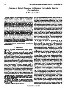
II. ATMOSPHERIC O CCLUDED F RONTS IN SAR I MAGES Occluded fronts are characterized by winds blowing in the opposite directions across the front. Within the transition area of the occluded front, surface wind fields are typically low, displayed as the low roughness or darker areas in SAR imagery. Fig. 1 is a collection of four ocean surface wind images derived from SAR sensors onboard both the Radarsat-1 and Envisat satellites. The image parameters are given in Table I. In Fig. 1, the color represents the ocean surface wind magnitudes. The measured NRCS is a function of wind speed, direction and satellite viewing angles. To derive ocean surface wind speed, one must obtain the wind direction from an independent source, i.e., operational numerical model or from wind-aligned features within the image. In this paper, the NOAA Global Forecast System (GFS) wind direction is used as input to the CMOD5 geophysical model function to calculate ocean surface wind speed at each pixel and then the wind is averaged to 500 m resolution [30]. The winds barbs shown in Fig. 1 are derived from the GFS model output at the nearest hour of the SAR imaging time. GFS provides hourly wind direction and speed data on a 0.5◦ × 0.5◦ longitude–latitude grid. The SAR wind retrievals have been very well validated against scatterometer and NOAA National Data Buoy Center (NDBC) marine buoy measurements. The wind speed standard deviation was calculated from the SAR-scatterometer or SAR-buoy matchups and has been found to be less than 2 m/s [31], [32]. The common characteristic is that there exists an elongate low-wind zone (low NRCS) in every image. It is clear that the winds on both sides of the front are in opposite directions. The lowwind zones are sometimes as wide as 100 km in Fig. 1(a) and (d) or as narrow as less than 10 km in Fig. 1(b) and (c). These observations were common features appearing in the high-latitude regions during all seasons. Occluded fronts are typically over 500 km long. The wind is asymmetric across the occluded front. Fig. 1(a) shows that the wind to the south of the front is much higher than that to the north of the front. Fig. 1(b) and (d) shows that the wind speeds are approximately at the same level on both sides of the lowwind speed zone. Fig. 1(c) shows there is a narrow high-wind band that is parallel to the occluded front. These observations demonstrate the occluded front occur under a wide range of atmospheric conditions.
LI et al.: SYNERGISTIC USE OF SATELLITE OBSERVATIONS AND NUMERICAL WEATHER MODEL
5271
Fig. 1. Four SAR-derived ocean surface wind images showing the atmospheric occluded fronts. (a) Radarsat-1 18:31 UTC, 06 March 2006. (b) Envisat 13:47 UTC, 10 March 2012. (c) Radarsat-1 18:20 UTC, 12 February 2005. (d) Radarsat-1 03:15 UTC, 24 September 2006. TABLE I BASIC C HARACTERISTICS OF THE F IVE SAR I MAGES (F IGS . 1 AND 2) U SED IN T HIS S TUDY
November 24, 2011. The Envisat WSM SAR has a pixel spacing of 75 m or a nominal spatial resolution of 150 m. The image covers about 450 km × 450 km horizontal area with the center located at about 51.5◦ N, 130.5◦ W. The eastern part of the image covers the part of the coast of British Columbia, Canada and the northern part of the image contains Haida Gwaii. Fig. 2(b) is an ocean surface wind image derived using the same procedures as followed in generating Fig. 1. Within the occluded front, the wind speed is less than 10 m/s, which is significantly lower than the wind speed outside the front, which is 30 m/s. The front is narrower to the north toward the center of the lowpressure system at about 55 km and widens to the south at about 65 km. B. Ocean Surface Winds Associated With an Occluded Front Observed by ASCAT
III. C ASE S TUDY W ITH M ULTIPLE S ATELLITE O BSERVATIONS AND S URFACE A NALYSIS A. SAR Observations of an Occluded Front on Nov. 24, 2011 Fig. 2(a) is an Envisat wide-swath mode (WSM) vertical polarization (VV) image acquired at 19:09 UTC on
The same front was also appeared in ASCAT imagery collected by the European Space Agency’s (ESA) polar-orbiting MetOp-A platform. The MetOp-A carries two sets of three vertically polarized C-band radar antennas that provide daily ocean surface wind measurements over 70% of the ice-free oceans in a dual-fan beam configuration. Instrument cross-track illumination coverage is nearly 550 km for each swath, separated by an approximate 700-km subtrack gap [33]. We obtained the Level2 product (12.5-km resolution) from the ESA/EUMETSAT
5272
IEEE TRANSACTIONS ON GEOSCIENCE AND REMOTE SENSING, VOL. 53, NO. 9, SEPTEMBER 2015
Fig. 3. ASCAT scatterometer wind image acquired at 18:12 UTC on November 24, 2011.
ASCAT data is wider than that in the SAR image. This indicates that the frontal zone was getting narrower as the cold front was catching up to the warm front in space and time. There are no near-shore wind retrievals from ASCAT due to the large footprint of the instrument. C. NOAA Surface Maps Analyses
Fig. 2. (a) and (b) ENVISAT SAR image acquired at 19:09 UTC on November 24, 2011 and the derived sea surface wind image. The GFS model wind directions are used as inputs to calculate the wind speed from calibrated SAR NRCS values.
Ocean and Sea Ice Satellite Application Facility (OSI SAF) through the KNMI FTP server. ASCAT measurements of ocean surface winds (Fig. 3) were made at 18:12 UTC, about 1 h before the SAR measurements were made, and are presented in Fig. 2(b). The wind patterns observed in ASCAT scatterometer and by SAR are very similar. The occluded front is shown as a low-wind zone in both observations. ASCAT scatterometer can measure both wind speed and direction, so the wind barbs shown in Fig. 3 are from the scatterometer measurement. Wind directions are consistent with the GFS numerical model results, as shown in Fig. 2(b). The wind speeds from scatterometer and SAR are not exactly the same. In the low-wind speed zone and in the north-western region, the SAR and scatterometer winds agree well. However, in the south-western regions, the SAR winds are more than 5 m/s higher than the scatterometer wind speeds. The discrepancies may due to system errors, time difference and retrieval errors. The ASCAT ocean surface wind observation was made about 1 h prior to the SAR observation. The low-wind zone in the
NOAA National Centers for Environmental Prediction (NCEP) surface analysis weather charts show the locations of synoptic scale high- and low-pressure centers with associated surface fronts and troughs for specific analysis times every 3 h The NCEP surface maps at 18:00 UTC (color) and 21:00 UTC (gray) on the same day as the SAR observation are overlaid in Fig. 4. The SAR coverage (Fig. 2) is shown as the box in Fig. 4. The map is presented in Lambert Projection. A frontal system associated with a low pressure system is apparent in Fig. 4. The cold front, warm front and occluded front are marked in blue, red and purple, respectively. The frontal system moved to the east and center of the low pressure system became smaller. It appears that the SAR imagery only covers the northern part of the entire occluded front. In situ ship wind measurements denoted as wind barbs in the surface chart, showed that the surface winds were predominately geotropic, and were blowing in the direction such that the high pressure is to the right-hand side. To the east (west) side of the occluded front, the wind was blowing to the north (south). The squeezing and lengthening of the occluded front was clear as it moved toward the east between 18:00 and 21:00 UTC. One can also see that the cold front moved faster than did the warm front during the same period. Note that the occlusion process occurred at ∼ 6:00 UTC and then the occluded front moved eastward and passed the location of the SAR and ASCAT observations. The cold front was entirely wrapped around the warm front and merged with the occluded front at 0:00 UTC on November 25 (surface map not shown for brevity). These observations matched with the conventional occlude process theory.
LI et al.: SYNERGISTIC USE OF SATELLITE OBSERVATIONS AND NUMERICAL WEATHER MODEL
5273
Fig. 4. Overlay of NOAA surface analysis maps at 18 UTC (color) and 21 UTC (grayscale). The map is in Lambert projection. The right panel shows the zoom map in the study region. TABLE II C OVERAGE OF THE T HREE N ESTED D OMAINS U SED IN THE WRF S IMULATION
D. WRF Model Simulation Results The WRF simulation was performed with Version 3.4 of the WRF, which is a fully compressible conservative-form nonhydrostatic atmospheric model, which was developed to be suitable for both research and weather-prediction applications that has demonstrated ability for resolving small-scale phenomena and clouds [34], [35]. A three-domain (triply) nested WRF configuration was employed, with 9-, 3-, and 1-km spatial resolutions, respectively, from the outermost to innermost domains. The coverage of the three nested domains is given in Table II. The innermost domain covers most of the occluded front. All model domains have 27 vertical layers, and the model top is set at 50 hPa. The WRF has multiple options for physical process parameterizations and the following parameterizations were chosen for this study: a) the Dudhia [36] shortwave and Rapid Radiative Transfer Model (RRTM) with long-wave radiation schemes; b) the Monin–Obukhov surface layer scheme; c) the Yonsei University Planetary Boundary Layer (YSU PBL) scheme [37]; d) the updated Kain-Fritsch cumulus scheme [38] for the outermost and second domains but not for the innermost domain; e) the WRF single-moment 3-class for cloud micro-
physics [39]; and f) the Noah land surface scheme [40], [41]. The GFS operational analyses and forecasts were employed for the model’s initial and boundary conditions. The experiment was performed for a 24-h simulation starting at 00:00 UTC on November 24, 2011. The GFS operational analyses are used for initial conditions, and the outermost coarse mesh lateral boundary conditions are specified by linearly interpolating these analyses. Fig. 5 shows the WRF 3.4 model-simulated surface wind and pressure fields at 18:00, 19:00, and 20:00 UTC. The plots at 18:00 and 19:00 UTC show that the low-wind field zone within the occluded front matched very well with ASCAT wind measurements taken at 18:12 UTC (cf. Fig. 3) and SARderived winds at 19:09 UTC (cf. Fig. 2). The low surface wind zone (within the occluded front) was squeezed over time and this process is consistent with the observations. At 18:00 UTC, there was a clear low-pressure center in Fig. 5 and this center disappeared in the subsequent pressure fields indicating that the system was weakening as the system moved to the east. The wind speed on the forward side of the occluded front weakened more than it did on the backward side as the center pressure dropped. Note that the pressure drop associated with the occluded front for this case follows the conventional wisdom of the Norwegian cyclone model presented by Bjerknes and Solberg 1922 [1]. In Fig. 6(a), we show a vertical cross section of potential temperature and wind at 19:00 UTC along the A-B line in Fig. 5(b). Below 800 mb, cold air descends strongly from the south and the warm air rises slowly in the north. The horizontal gradient of the potential temperature is the largest when the downward motion becomes upward. Front occlusion occurs at the location of this largest horizontal temperature gradient. Because the air behind the cold front is much colder than the air ahead of the warm front, this occluded front is a coldtype front following the conventional wisdom of the Norwegian cyclone model [1] and the temperature rule [4]. However, Stoelinga et al. [4] also pointed out that the temperature rule does not explain the structure of the occluded fronts and argued
5274
IEEE TRANSACTIONS ON GEOSCIENCE AND REMOTE SENSING, VOL. 53, NO. 9, SEPTEMBER 2015
Fig. 5. (a)–(f) WRF surface wind and pressure field from WRF model simulation at 18, 19, and 20 UTC.
that the relative stability on either side of the occluded front determines the type and structure of the occluded front (i.e., the static-stability rule). If the air behind the cold front is less stable than the air ahead of the warm front, the occluded front is regarded as a warm-type occluded front. If the air behind the cold front is more stable than the air ahead of the warm front, the occluded front is regarded as a cold-type. Fig. 6(b) shows the vertical cross section of the static stability along the A-B line in Fig. 5(b). It appears that the low-level air (below 800 mb) on the side of the cold front is more stable than the air on the warm cold front. Fig. 5(a) and (b) indicate that occlusion formed from
lifting the less stable air from the zone of warm front over the more stable air at the cold front zone. This structure indicates that the occluded front is a typical cold-type occluded front based on the stability rule. Although, it is rare to observe coldtype front because cold-frontal zones are less likely to be more statically stable than warm-fontal zones [6], our study presented another case for cold-type occlusion following a recent study by Schultz et al. [42] who documented the first case in the literature [42]. To study the evolution of the detailed structure as the occluded front passed the region of SAR and ASCAT
LI et al.: SYNERGISTIC USE OF SATELLITE OBSERVATIONS AND NUMERICAL WEATHER MODEL
5275
Fig. 7. Three-dimensional view of WRF-simulated potential temperature (a, b, and c) and specific humidity (d, 497 e, f) at 15, 18, and 21 UTC. Fig. 6. Vertical potential temperature (θ)/horizontal wind (full barb, and halfbarb denote 10 and 5 m/s, respectively) profiles (a) and d(θ)/dZ (b) along line a-B in Fig. 5(d) from WRF 494 simulation at 19 UTC.
observations, Fig. 7 presents a 3-D view of time series of WRF-simulated potential temperatures (a, b, c) and specific humidity (d, e, f) at 15:00, 18:00, and 21:00 UTC on November 24. It demonstrates that the cold air mass pushed the southern boundary of the warm air mass from 133◦ W at 15:00 UTC to 131◦ W at 18:00 UTC and then 129◦ W at 21:00 UTC. At the same time, dry air associated with the cold air mass wrapped up the moist air and moved to the low pressure center. It also shows that the occlusion process happened mostly below the 800-mb level. This occlusion process is consistent with the new paradigm proposed by Schultz and Vaughan, [11] in that the cold front tends to wrap up the warm front (see [6, Figs. 14 and 17]). The general precipitation pattern associated with the occluded front is that it typically occurs on the warm air side of the occlusion and then wraps around the warm air mass and moves toward the low-pressure center following the occlusion [6]. The WRF simulated hourly precipitation rates at 15:00, 18:00 and 21:00 UTC are overplotted on contemporaneous NOAA surface maps as shown in Fig. 8. Our WRF domain only covers the occluded frontal region, and not the entire cold and warm frontal regions, during the 24-h simulation. The rain patterns are clearly shown in the northwest side of the low-pressure center, which is associated with the occluded
front at 18:00 and 21:00 UTC. Schultz and Vaughan [6] pointed out in their new paradigm for the occluding process that intense precipitation occurs following formation of the occluded front. Our WRF simulation supports this paradigm. In addition, the precipitation shown in the location of the SAR observation, weakened after the passage of the occluded front, a finding that is also consistent with the previous observational studies [3], [43]. IV. C ONCLUSION Occluded front is one of the most common of weather systems. Although numerous studies of occluded fronts have been reported on in the peer-reviewed literature, observations from space of its surface signatures are unique. The SAR satellite observations of atmospheric occluded frontal reveal many types of sea surface imprints of occluded front as shown in Fig. 1. The lengths and widths of the occluded fronts are shown to vary significantly. The SAR-derived surface winds show that there is usually a low-wind zone within the occluded front, whereas the winds outside this zone are sometimes but not always symmetric in amplitude and blow in opposite directions to those winds in the frontal zone per se. Often times the winds outside of the occluded front are asymmetric with stronger winds on one side and weaker winds on the other. A case study shows that in one manifestation of an occluded front, the cold air did not wrap around the low pressure center
5276
IEEE TRANSACTIONS ON GEOSCIENCE AND REMOTE SENSING, VOL. 53, NO. 9, SEPTEMBER 2015
Fig. 8. WRF-simulated hourly accumulated rain rate at 15(a), 18(b), and 21(c) on November 24, 2011. The rain rate maps in color are overplotted on the corresponding NOAA surface analysis maps. Zoomed maps are shown on the left panels.
at 18:00 (scatterometer) and 19:00 (SAR) UTC. The circulation near the low-pressure center was not very strong. There is a clear central low-wind zone (< 10 m/s, Fig. 2(b) with higher winds (> 25 m/s) blowing in a direction opposite to that of the weaker winds within the front and on both lateral sides of the front. This whole process was recaptured by employing a triply
nested WRF numerical model. The WRF model simulation shows that the process of occluding is a cold-type occlusion according to both the temperature and the static stability rules, and the occlusion process happened below the 800-mb level. The occluded front moved toward the east during the 24-h model simulation, and the movement between 18:00 and 21:00
LI et al.: SYNERGISTIC USE OF SATELLITE OBSERVATIONS AND NUMERICAL WEATHER MODEL
UTC matched the frontal positions from the NCEP surface weather maps during the same period. Low-level wind, potential temperature, specific humidity and precipitation results from WRF model simulation also confirm the relatively new findings presented by Schultz and Vaughan [6]. High-resolution SAR helped our analysis in twofolds: 1) the resolution of SAR and WRF model is comparable. Therefore, by analyzing the wind pattern simulated by the WRF model and acquired by SAR, we have confidence in further analyzing the time series of model results. 2) SAR-derived wind field is also a good validation for model run results. For the first time, this study demonstrates that synergy SAR, scatterometer observation as well as community WRF simulation to reveal the generation and evolution of an occluded front. This study also adds to the body of scholarly evidence of the synergy that exists between satellite SAR and comparable high spatial resolution community weather forecast models to study atmospheric phenomena including but not limited to: katabatic winds [11], atmospheric vortex streets [21], atmospheric gravity waves and boundary layer rolls [16], [17], [43]. With the rapid advance of community atmospheric mesoscale numerical modeling capabilities, we have demonstrated that the high resolution WRF model could be an ideal tool to study SARobserved atmospheric phenomena in the MABL. ACKNOWLEDGMENT This paper is in final form on the last day of coauthor William (Bill) Pichel’s working day with NOAA before his retirement. W. Pichel’s 45 years of leadership and dedication to NOAA ocean remote sensing program will be truly missed. X. Li acknowledges all the support, encouragement, and trust from W. Pichel during the past 18 years. W. Pichel wins not only the Distinguished Career Award and a Gold Medal from NOAA, but also a Gold Medal for life from all of us who had the privilege to work with him. The Envisat Advanced SAR image was provided by the European Space Agency under Envisat Projects 19011 and 6133. ASCAT Level-2 wind data are obtained from: http://www.eumetsat.int/. The views, opinions, and findings contained in this report are those of the authors and should not be construed as an official NOAA or U.S. Government position, policy, or decision. R EFERENCES [1] J. Bjerknes and H. S. Solberg, Life Cycle of Cyclones and the Polar Front Theory of Atmospheric Circulation. Oslo, Norway: Geophysisks Publikationer, 1922. [2] D. Keyser, “Atmospheric fronts: An observational perspective,” in Mesoscale Meteorology and Forecasting, P. S. Ray, Eds. Boston, MA, USA: Amer. Meteorol. Soc., 1986, pp. 216–258. [3] D. M. Schultz and C. F. Mass, “The occlusion process in a midlatitude cyclone over land,” Mon. Weather Rev., vol. 121, no. 4, pp. 918–940, Apr. 1993. [4] M. T. Stoelinga, J. D. Locatelli, and P. V. Hobbs, “Warm occlusions, cold occlusions, and forward-tilting cold fronts,” Bull. Amer. Meteorol. Soc., vol. 83, no. 5, pp. 709–721, May 2002. [5] D. M. Schultz and F. Q. Zhang, “Baroclinic development within zonally-varying flows,” Q. J. R. Meteorol. Soc., vol. 133, no. 626, pp. 1101–1112, Jul. 2007. [6] D. M. Schultz and G. Vaughan, “Occluded fronts and the occlusion process a fresh look at conventional wisdom,” Bull. Amer. Meteorol. Soc., vol. 92, no. 4, pp. 443–466, Apr. 2011.
5277
[7] L. L. Fu and B. Holt, “Some examples of detection of oceanic mesoscale Eddies by the Seasat synthetic-aperture radar,” J. Geophys. Res.: Oceans, vol. 88, no. C3, pp. 1844–1852, Feb. 1983. [8] D. Atlas, “Footprints of storms on the sea—A view from spaceborne synthetic-aperture radar,” J. Geophys. Res.: Oceans, vol. 99, no. C4, pp. 7961–7969, Apr. 15, 1994. [9] X. F. Li et al., “Tropical cyclone morphology from spaceborne synthetic aperture radar,” Bull. Amer. Meteorol. Soc., vol. 94, no. 2, pp. 215–230, Feb. 2013. [10] W. Alpers, U. Pahl, and G. Gross, “Katabatic wind fields in coastal areas studied by ERS-1 synthetic aperture radar imagery and numerical modeling,” J. Geophys. Res.: Oceans, vol. 103, no. C4, pp. 7875–7886, Apr. 15, 1998. [11] X. F. Li, W. H. Zheng, W. G. Pichel, C. Z. Zou, and P. Clemente-Colon, “Coastal katabatic winds imaged by SAR,” Geophys. Res. Lett., vol. 34, no. 3, pp. 1–5, Feb. 3, 2007. [12] P. W. Vachon, O. M. Johannessen, and J. A. Johannessen, “An ERS-1 synthetic-aperture-radar image of atmospheric lee waves,” J. Geophys. Res.: Oceans, vol. 99, no. C11, pp. 22483–22490, Nov. 15, 1994. [13] I. Chunchuzov, P. W. Vachon, and X. Li, “Analysis and modeling of atmospheric gravity waves observed in RADARSAT SAR images,” Remote Sens. Environ., vol. 74, no. 3, pp. 343–361, Dec. 2000. [14] X. F. Li, C. M. Dong, P. Clemente-Colon, W. G. Pichel, and K. S. Friedman, “Synthetic aperture radar observation of the sea surface imprints of upstream atmospheric solitons generated by flow impeded by an island,” J. Geophys. Res.: Oceans, vol. 109, no. C2, pp. 1–8, Feb. 17, 2004. [15] X. L. Gan et al., “Coastally trapped atmospheric gravity waves on SAR, AVHRR and MODIS images,” Int. J. Remote Sens., vol. 29, no. 6, pp. 1621–1634, 2008. [16] X. F. Li, W. Z. Zheng, X. F. Yang, Z. W. Li, and W. G. Pichel, “Sea surface imprints of coastal mountain lee waves imaged by synthetic aperture radar,” J. Geophys. Res.: Oceans, vol. 116, no. C2, pp. 1–10, Feb. 12, 2011. [17] X. F. Li et al., “Coexistence of atmospheric gravity waves and boundary layer rolls observed by SAR,” J. Atmos. Sci., vol. 70, no. 11, pp. 3448–3459, Nov. 2013. [18] W. Alpers and B. Brummer, “Atmospheric boundary-layer rolls observed by the synthetic-aperture radar aboard the ERS-1 satellite,” J. Geophys. Res.: Oceans, vol. 99, no. C6, pp. 12613–12621, Jun. 15, 1994. [19] G. Levy, “Boundary layer roll statistics from SAR,” Geophys. Res. Lett., vol. 28, no. 10, pp. 1993–1995, May 15, 2001. [20] X. F. Li, P. Clemente-Colon, W. G. Pichel, and P. W. Vachon, “Atmospheric vortex streets on a RADARSAT SAR image,” Geophys. Res. Lett., vol. 27, no. 11, pp. 1655–1658, Jun. 1, 2000. [21] X. F. Li, W. Z. Zheng, C. Z. Zou, and W. G. Pichel, “A SAR observation and numerical study on ocean surface imprints of atmospheric vortex streets,” Sens.-Basel, vol. 8, no. 5, pp. 3321–3334, May 2008. [22] A. Y. Ivanov et al., “Atmospheric front over the East China Sea studied by multisensor satellite and in situ data,” J. Geophys. Res.: Oceans, vol. 109, no. C12, Dec. 1, 2004. [23] G. S. Young, T. N. Sikora, and N. S. Winstead, “Use of synthetic aperture radar in finescale surface analysis of synoptic-scale fronts at sea,” Weather Forecast, vol. 20, no. 3, pp. 311–327, Jun. 2005. [24] G. Young, T. Sikora, and N. Winstead, “Mesoscale near-surface wind speed variability mapping with synthetic aperture radar,” Sens.-Basel, vol. 8, no. 11, pp. 7012–7034, Nov. 2008. [25] S. Ufermann and R. Romeiser, “Numerical study on signatures of atmospheric convective cells in radar images of the ocean,” J. Geophys. Res.: Oceans, vol. 104, no. C11, pp. 25707–25719, Nov. 15, 1999. [26] S. M. Babin, T. D. Sikora, and N. S. Winstead, “A case study of satellite synthetic aperture radar signatures of spatially evolving atmospheric convection over the Western Atlantic Ocean,” Boundary Layer Meteorol., vol. 106, no. 3, pp. 527–546, Mar. 2003. [27] R. Romeiser et al., “On the remote sensing of oceanic and atmospheric convection in the Greenland Sea by synthetic aperture radar,” J. Geophys. Res.: Oceans, vol. 109, no. C3, pp. 1–14, Mar. 2, 2004. [28] T. D. Sikora, G. S. Young, C. M. Fisher, and M. D. Stepp, “A synthetic aperture radar-based climatology of open-cell convection over the Northeast Pacific Ocean,” J. Appl. Meteorol. Clim., vol. 50, no. 3, pp. 594–603, Mar. 2011. [29] J. Dudhia et al., “A collaborative effort towards a future community mesoscale model (WRF),” in Proc. 12th Conf. Numerical Weather Prediction, 1998, pp. 242–243. [30] H. Hersbach, A. Stoffelen, and S. de Haan, “An improved C-band scatterometer ocean geophysical model function: CMOD5,” J. Geophys. Res.: Oceans, vol. 112, no. C3, pp. 1–18, Mar. 6, 2007.
5278
IEEE TRANSACTIONS ON GEOSCIENCE AND REMOTE SENSING, VOL. 53, NO. 9, SEPTEMBER 2015
[31] X. F. Yang, X. F. Li, W. G. Pichel, and Z. W. Li, “Comparison of ocean surface winds from ENVISAT ASAR, MetOp ASCAT scatterometer, Buoy measurements, and NOGAPS model,” IEEE Trans. Geosci. Remote, vol. 49, no. 12, pp. 4743–4750, Dec. 2011. [32] X. F. Yang et al., “Comparison of ocean-surface winds retrieved from QuikSCAT scatterometer and Radarsat-1 SAR in offshore waters of the U.S. West Coast,” IEEE Geosci. Remote Sens. Lett., vol. 8, no. 1, pp. 163–167, Jan. 2011. [33] J. Verspeek et al., “Validation and calibration of ASCAT using CMOD5.n,” IEEE Trans. Geosci. Remote, vol. 48, no. 1, pp. 386–395, Jan. 2010. [34] C. Davis et al., “Prediction of landfalling hurricanes with the advanced hurricane WRF model,” Mon. Weather Rev., vol. 136, no. 6, pp. 1990–2005, Jun. 2008. [35] H. L. Wang, W. C. Skamarock, and G. Feingold, “Evaluation of scalar advection schemes in the advanced research WRF model using large-Eddy simulations of aerosol-cloud interactions,” Mon. Weather Rev., vol. 137, no. 8, pp. 2547–2558, Aug. 2009. [36] J. Dudhia, “Numerical study of convection observed during the winter monsoon experiment using a mesoscale two-dimensional model,” J. Atmos. Sci., vol. 46, no. 20, pp. 3077–3107, Oct. 15, 1989. [37] S. Y. Hong, Y. Noh, and J. Dudhia, “A new vertical diffusion package with an explicit treatment of entrainment processes,” Mon. Weather Rev., vol. 134, no. 9, pp. 2318–2341, Sep. 2006. [38] J. S. Kain, “The Kain-Fritsch convective parameterization: An update,” J. Appl. Meteorol., vol. 43, no. 1, pp. 170–181, Jan. 2004. [39] S. Y. Hong, J. Dudhia, and S. H. Chen, “A revised approach to ice microphysical processes for the bulk parameterization of clouds and precipitation,” Mon. Weather Rev., vol. 132, no. 1, pp. 103–120, Jan. 2004. [40] F. Chen and J. Dudhia, “Coupling an advanced land surface-hydrology model with the Penn State-NCAR MM5 modeling system. Part I: Model implementation and sensitivity,” Mon. Weather Rev., vol. 129, no. 4, pp. 569–585, Apr. 2001. [41] M. B. Ek et al., “Implementation of Noah land surface model advances in the National Centers for Environmental Prediction operational mesoscale Eta model,” J. Geophys. Res.: Atmos., vol. 108, no. D22, pp. 12-1–12-16, Nov. 29, 2003. [42] D. M. Schultz, B. Antonescu, and A. Chiariello, “Searching for the elusive cold-type occluded front,” Mon. Weather Rev. vol. 142, no. 8, pp. 2565–2570, Aug. 2014. [43] N. S. Winstead, G. S. Young, and T. D. Sikora, “Determined wind speed in numerical weather prediction error detection,” Nat. Weather Dig. vol. 36, no. 2, pp. 69–80, 2012.
Xiaofeng Li (M’00–SM’11) received the B.S. degree in optical engineering from Zhejiang University, Hangzhou, China, in 1985; the M.S. degree in physical oceanography from the First Institute of Oceanography, State Oceanic Administration, Qingdao, China, in 1992; and the Ph.D. degree in physical oceanography from North Carolina State University, Raleigh, NC, USA, in 1997. During the M.S. program, he completed the graduate course work at the Department of Physics, University of Science and Technology of China, Hefei, China. Since 1997, he has been with the National Oceanic and Atmospheric Administration/National Environmental Satellite, Data, and Information Service (NESDIS), College Park, MD, USA. He is involved in developing many operational satellite ocean remote sensing products at NESDIS. His research interests include remote sensing observation and theoretical/numerical model studies of various types of oceanic and atmospheric phenomena, satellite image processing, ocean surface oil spill and target detection/classification with multipolarization SAR, and sea surface temperature algorithms development. He is an author of more than 100 peer-reviewed publications and the chief editor of Remote Sensing of the China Seas (Taylor & Francis, 2014) and Maritime Oil Spill Response (Elsevier, 2015). Dr. Li has served as the Associate Editor for the International Journal of Remote Sensing since 2013. He is also an editorial board member for the International Journal of Digital Earth and Acta Oceanologica Sinica. He was appointed as an “Overseas Expert” by the Chinese Academy of Sciences in 2014.
Xiaofeng Yang (S’07–M’11) received the B.S. degree in environmental science from Sichuan University, Chengdu, China, in 2005 and the Ph.D. degree in cartography and geographic information systems from the Institute of Remote Sensing Applications (IRSA), Chinese Academy of Sciences (CAS), Beijing, China, in 2010. During his Ph.D. program, 2009–2010, he was a Visiting Research Scientist with the Department of Atmospheric and Oceanic Science, University of Maryland, College Park. From 2010 to 2012, he was an Assistant Researcher at IRSA/CAS. Since 2013, he has been with RADI/CAS as an Associate Researcher. His research interests include satellite oceanography, synthetic aperture radar image processing, and marine atmospheric boundary layer process studies. He has also participated in the development of various types of operational ocean products in China coastal waters from environmental satellite data. He has also served as a reviewer of several international academic journals.
Weizhong Zheng received professional training from the Department of Atmospheric Sciences, Nanjing University of China, where he obtained the B.S. degree in 1982, the M.S. degree in 1985, and the Ph.D. degree in 1999. Since 1985, he has worked at Nanjing University, University of L’Aquila of Italy and University of Maryland. He joined at National Oceanic and Atmospheric Administration (NOAA)/NESDIS as a scientist in 2002 and then moved to NOAA/NCEP/Environmental Modeling Center in 2007. His research interests focus on numerical weather prediction and data assimilation, including development and improvement of parameterizations of physical processes in the numerical models as well as monitoring and improvement of satellite data utilization over land in NCEP operational numerical weather prediction modeling and data assimilation systems. He is an author of tens of peer-reviewed publications.
Jun A. Zhang (M’00–SM’11) received the B.S. degree in naval architecture and ocean engineering from the Dalian University of Technology, Liaoning, China, in 2000; the M.S. degree in applied marine physics from the Rosenstiel School of Marine and Atmospheric Science, University of Miami, FL, USA, in 2005; and the Ph.D. degree in applied marine physics from the Rosenstiel School of Marine and Atmospheric Science, University of Miami, FL, USA, in 2007. Since 2008, he has been with the National Oceanic and Atmospheric Administration/Atlantic Oceanographic and Meteorological Laboratory/Hurricane Research Division, Miami, FL, USA. He is involved in hurricane field experiments at HRD. He is also involved in improving hurricane model physics using aircraft data. His research interests include boundary layer structure and dynamics, turbulence, air– sea interaction, remote sensing, numerical modeling, and physical parameterizations. He is an author of more than 40 peer-reviewed publications. Dr. Zhang has served as the Associate Editor for Monthly Weather Review since 2013.
LI et al.: SYNERGISTIC USE OF SATELLITE OBSERVATIONS AND NUMERICAL WEATHER MODEL
Leonard J. Pietrafesa received the B.S. degree from Fairfield University, Fairfield, CT, USA, in 1965; the M.S. degree from Boston College/ University of Chicago (Boston, MA, USA/Chicago, IL, USA) in 1967; and the Ph.D. degree from the University of Washington, Seattle, WA, USA, in 1973. He was an Assistant (1973), Associate (1976), and Full Professor (1981) with North Carolina State University (NCSU), Raleigh, NC, USA. He was the Head of the Department of Marine, Earth and Atmospheric Sciences, between 1989 and 2000, the Executive Director and later Associate Dean of the Office of External Affairs and Associate Dean for Research of the College of Mathematical and Physical Sciences, NCSU between 2000 and 2008. He has been a Professor Emeritus, NCSU since 2008 and the Burroughs & Chapin Scholar, Coastal Carolina University, Conway, SC, USA since 2010. He was the cowriter of the U.S. Senate Bill for legislation and rewrite of U.S. House Bill in a Next-Generation Modernization of the U.S. National Weather Service (07/2014–03/2015). He was the Chair of the National Oceanic and Atmospheric Administration Science Advisory Board (FACA approved). He gave federal testimony twice before the U.S. Senate and seven times before the U.S. House of Representatives. He had also served as an Adviser for the North Carolina governors on coastal issues for 19 years. He has published more than 200 peer-reviewed papers, supervised 27 Ph.D. and 28 M.S. students and 17 Postdoctoral Fellows, and won 107 research awards totaling more than $28 million funding. Dr. Pietrafesa is an American Meteorological Society (AMS) Fellow, served on the Editorial Board of American Geophysical Union (AGU) EOS and was on the UCAR Board of Trustees.
5279
William G. Pichel (M’94) received the B.S. degree in physics from the University of Florida, Gainesville, FL, USA, in 1969 and the M.S. degree in physical oceanography from the University of Hawaii, Honolulu, HI, USA, in 1979. He began his career with the National Oceanic and Atmospheric Administration (NOAA) in 1970 as a NOAA Corps Officer. In 1973, he became a Civilian Employee with the National Environmental Satellite, Data, and Information Service (NESDIS). Past assignments have included Product Area Leader (PAL) for Oceanographic Products, PAL for Winds Products, and Chief of the Product Systems Branch. Since 1988, he has been a Physical Scientist with the Satellite Oceanography and Climatology Division, Center for Satellite Applications and Research (STAR), NOAA/NESDIS, where he is the Chair of the Sea Surface Roughness Science Team. His research interests are centered on development of coastal ocean applications of synthetic aperture radar (SAR) data. Mr. Pichel is a recipient of four Department of Commerce Bronze Medals for his work in sea surface temperatures and SAR, a Silver Medal for his work in marine debris detection at sea, a Gold Medal for helping to transition SARderived winds to operations, and the NOAA Distinguished Career Award for advancing the state-of-the-art of satellite operational ocean remote sensing.