Syntax and Semantics of Timed Chi - Semantic Scholar

Syntax and Semantics of Timed Chi

D.A. van Beek1 , K.L. Man2 , M.A. Reniers2 , J.E. Rooda1 , R.R.H. Schiffelers1 1 Department of Mechanical Engineering 2 Department of Mathematics and Computer Science Eindhoven University of Technology, P.O.Box 513 5600 MB Eindhoven, The Netherlands {d.a.v.beek,k.l.man,m.a.reniers,j.e.rooda,r.r.h.schiffelers}@tue.nl

ii

Contents 1

Introduction

1

2

Syntax and informal semantics of the timed Chi language

5

2.1

Processes . . . . . . . . . . . . . . . . . . . . . . . . . . . . . . . . . . . . .

5

2.2

Process terms . . . . . . . . . . . . . . . . . . . . . . . . . . . . . . . . . . .

6

2.3

Syntactic extensions . . . . . . . . . . . . . . . . . . . . . . . . . . . . . . . .

10

2.4

Data types . . . . . . . . . . . . . . . . . . . . . . . . . . . . . . . . . . . . .

16

3

Semantics of the timed Chi language

17

3.1

General description of the SOS . . . . . . . . . . . . . . . . . . . . . . . . . .

17

3.2

Notations and mathematical definitions

. . . . . . . . . . . . . . . . . . . . .

19

3.3

Deduction rules for atomic process terms . . . . . . . . . . . . . . . . . . . .

21

3.4

Deduction rules for operators . . . . . . . . . . . . . . . . . . . . . . . . . . .

22

4

Discrete-event model of a manufacturing line

33

5

Translating timed automata to timed Chi

37

5.1

Definition of a timed automaton . . . . . . . . . . . . . . . . . . . . . . . . .

37

5.2

General translation scheme . . . . . . . . . . . . . . . . . . . . . . . . . . . .

38

5.3

Example: a coffee vendor machine . . . . . . . . . . . . . . . . . . . . . . . .

39

6

Derivation of timed Chi from hybrid Chi

41

6.1

The L1 language . . . . . . . . . . . . . . . . . . . . . . . . . . . . . . . . .

41

6.2

The L2 language . . . . . . . . . . . . . . . . . . . . . . . . . . . . . . . . .

43

iii

Contents

iv

6.3

Relating L0 (∅, ∅) and L2 . . . . . . . . . . . . . . . . . . . . . . . . . . . . .

45

6.4

Relating L2 and timed Chi . . . . . . . . . . . . . . . . . . . . . . . . . . . .

46

7 Validation of the semantics

47

7.1

Well-definedness of the semantics . . . . . . . . . . . . . . . . . . . . . . . .

47

7.2

Properties of the semantics . . . . . . . . . . . . . . . . . . . . . . . . . . . .

47

7.3

Stateless bisimilarity . . . . . . . . . . . . . . . . . . . . . . . . . . . . . . .

49

7.4

Properties of the Chi operators . . . . . . . . . . . . . . . . . . . . . . . . . .

51

Bibliography

53

A Derivation of DL2 from DL1

55

A.1 Derivation for atomic process terms . . . . . . . . . . . . . . . . . . . . . . .

55

A.2 Derivation for operators . . . . . . . . . . . . . . . . . . . . . . . . . . . . . .

58

Chapter 1

Introduction In this document, the timed χ (Chi) language is described. The timed χ language is obtained by means of simplification of hybrid χ (see [17]). The intended use of χ is for modeling, simulation, verification, and real-time control. Its application domain consists of large and complex manufacturing systems. Although the semantics is formally defined, the straightforward and elegant syntax and semantics is also highly suited to non-computer scientists. In the remainder of this report, we usually refer to timed χ as χ. The most important concepts in χ are summarized below: 1. Integration of a straightforward semantics and ease of modeling. • Strong time deterministic alternative composition operator. Where in the previous version of discrete-event χ [5] the passage of time could result in making a choice between the two operands of the alternative composition operator (weak time determinism), as is the case in many process algebras, in the current χ semantics, the passage of time can never result in such a choice. In fact, the passage of time can only result in changes to the value of the predefined variable time. In the previous versions of χ, alternative composition 15 [] x := 1 could non-deterministically choose between doing a delay of t ≤ 5 to 1(5 − t), or doing the (undelayable) action x := 1 and then terminate. Strong time deterministic alternative composition means that alternative composition can delay only if both process terms can delay together, so that 15 [] x := 1 can only do the (non-delayable) action x := 1, and then terminate. Timed automata have a comparable choice mechanism, apart from initialization. In a timed automaton, action transitions cannot disappear as a result of time passing. They can only be disabled for the period of time that the associated guard evaluates to false in the valuation prescribed by the trajectory of the variables. Also, time passing cannot result in the choice of a different location. The only changes in a timed automaton as a result of time passing are changes in the values of the clocks. Only initially, depending on the initial edges and invariants, different initial locations may be selected as a result of time passing.

1

Chapter 1. Introduction

2

• Delayable guards. Where the previous version of discrete-event χ [5] had nondelayable guards, such as found in many process algebras, the current χ semantics has delayable guards. A non-delayable guard cannot perform a delay when it is false. A delayable guard can delay when it is false until it becomes true, and thus facilitates modeling. Consider for example a valve α that must be switched on when the time becomes bigger then tmax . Using a delayable guard, this can be modeled simply by time ≥ tmax → α := true. Delayable guards ensure that in b → h ! b, the value of expression b that is sent via channel h is always true. Note that h ! b can either do a send action, or delay for an arbitrary period of time. Non-delayable guards may lead to un-intuitive behavior, because the value of b that is sent may be false. Consider the process term: ((time ≤ 3 → h ! time) [] 110) || 15; h ? y. Using non-delayable guards, the process term can perform a delay of at most 5, and after performing an internal action transforms into (h ! time [] 15) || h ? y. The guard that was true has disappeared in delaying. If the communication via channel h takes place now, a value of 5 is sent, which does not conform to time ≤ 3. Using delayable guards on the other hand, the process term can do the delay of at most 3, and transforms into: (time ≤ 3 → h ! time [] 17) || 12; h ? y, where the value of time is 3. Communication is still not possible. After a delay of 2, followed by an internal action, the process term transforms into: (time ≤ 3 → h ! time [] 15) || h ? y, where the value of time is 5, and after another delay of 5 it transforms into: (time ≤ 3 → h ! time [] 10) || h ? y. The time-out takes place, leading to: h ? y. Due to the delayable guard, that does not disappear while delaying, the communication does not take place, because the guard cannot be satisfied. • Integrated urgent and non-urgent actions. The χ formalism has both urgent and non-urgent actions. The concept of urgency is defined in a very flexible way: nondelayable actions are by definition urgent and delayable actions are non-urgent. This is achieved without any additional operators. A maximal progress operator as defined in [5] is not needed. The concept of urgency is built into the individual parallel composition, alternative composition and guard operators. Consider the non-delayable action x := 1. The following three process terms

3

– – –

15 || x := 1 15 [] x := 1 time = 0 y (time ≤ 0 → x := 1)

can each execute only the action x := 1. Here, time = 0 y p denotes a process term p for which the value of time is initially zero. Consider now the delayable action [x := 1]. The following three process terms – – –

15 || [x := 1] 15 [] [x := 1] time = 0 y (time ≤ 0 → [x := 1])

can each execute either the action x := 1 or perform a delay. This concept is comparable to so-called urgent transitions that are present in, for example U PPAAL [8]. Communication on channels can also be urgent and non-urgent as in U PPAAL. This is achieved by means of an operator that partitions the set of channels into a set of urgent and a set of non-urgent channels. For the urgent channels, communication must take place as soon as it becomes possible, whereas for the non-urgent channels, no such preference for communication is assumed. • Syntactic extensions. Ease of modeling is further supported in χ by extension of the small set of orthogonal core process terms with additional process terms for ease of modeling. These additional process terms are defined by means of a straightforward mapping into the core process terms. 2. Concepts for complex system specification. • Process terms for scoping that integrate abstraction, local variables, local channels and recursion definitions. • Parameterized process definition and process instantiation that enable: – process re-use and – encapsulation, hierarchical and/or modular composition of processes. • CSP communication and synchronization concepts that allow synchronization and communication without sharing of variables. The history of the χ language dates back quite some time. It was originally designed as a modeling and simulation language for specification of discrete-event, continuous-time or combined discrete-event/continuous-time models. The first simulator [13] was suited to discrete-event models only. The simulator was successfully applied to a large number of industrial cases, such as an integrated circuit manufacturing plant, a brewery, and process industry plants [19]. Later, the hybrid language and simulator were developed [7, 18]. For the purpose of verification, the discrete-event part of the language was mapped onto the process algebra χσ by means of a syntactical translation. The semantics of χσ was defined using a structured operational semantics style (SOS), bisimulation relations were derived, and a model checker was built [5]. In this way, verification of discrete-event χ models was made possible [4]. In [17], the hybrid χ language

4

Chapter 1. Introduction

was formally defined. The timed χ language described in this report is obtained as a simplification of hybrid χ. It is suited for discrete-event modeling. Where in χσ , it was not possible to refer to the current (model) time, in timed χ, there is a predefined variable time, that denotes the current time. This report is organized as follows. Chapter 2 describes the syntax and informal semantics of the timed χ language. In Chapter 3, the semantics of timed χ is formally specified. An example in Chapter 4 illustrates the use of the language. A general translation scheme for translating timed automata to timed χ is given in Chapter 5. The derivation of timed χ from hybrid χ is described in Chapter 6. In Chapter 7, a notion of equivalence is defined, which is shown to be a congruence for all timed χ operators. Furthermore, some useful properties of closed timed χ process terms are given.

Chapter 2

Syntax and informal semantics of the timed Chi language This chapter presents a concise definition of the syntax and informal semantics of timed χ. The syntax definition is incomplete in the sense that the syntax of predicates, expressions, etc, is not defined. In the remainder of this report, we usually refer to timed χ as χ.

2.1 Processes A χ process is a triple h p, σ, Ei, where p denotes a process term, σ denotes a valuation, and E denotes an environment. The syntax of process terms is introduced in Section 2.2. Variables in χ are used to store information, i.e., during execution variables have a value. A valuation is a partial function from variables to values. Syntactically, a valuation is denoted by a set of pairs {x0 7 → c0 , . . . , xn 7 → cn }, where xi denotes a variable and ci its value. The valuation σ and the environment E, together define the variables that exist in the χ process and the variable classes to which they belong. Discrete behavior (instantaneous changes) of a χ process is represented by means of action transitions, and delay behavior (time passing) is represented by means of time transitions. The variables are grouped into different classes with respect to the delay behavior and the action behavior. With respect to the delay behavior, the variables are divided into the following classes: • The discrete variables, the values of which remain constant while delaying. • The predefined variable ‘time’, that denotes the current time. With respect to the action behavior, the variables are divided into two classes:

5

6

Chapter 2. Syntax and informal semantics of the timed Chi language

• The non-jumping variables, the values of which by default do not change during action transitions. Such changes need to be explicitly specified. This is the normal behavior of the χ variables. The predefined variable time is by definition non-jumping. • The jumping variables, the values of which by default can jump to arbitrary values in actions. The values after jumping can be restricted by means of the action predicate, or receive process term, that caused the jump. Note that in principle, jumping variables occur only as an artefact of the parallel composition of a send and a receive process term, where the receive process term assigns the received value to a discrete variable, see Sections 3.3.2 and 3.4.6. In χ, an environment is a tuple (J, R), where J denotes the set of jumping variables, and R denotes a recursive process definition. It is required that J ⊆ (dom(σ ) \ {time}), and dom(σ ) ∩ dom(R) = ∅. A recursive process definition is a partial function from recursion variables to process terms. Syntactically, a recursive process definition is denoted by a set of pairs {X 0 7 → p0 , . . . , X m 7 → pm }, where X i denotes a recursion variable and pi the process term defining it. The domain of the valuation σ in a χ process h p, σ, Ei consists of the discrete variables and the predefined variable time. For a χ process h p, σ, (J, R)i, the combination of the variable classes for the delay and action behavior leads to the following classes of variables: • The set of discrete variables D is dom(σ ) \ {time}. – the set of non-jumping discrete variables is D \ J , – the set of jumping discrete variables is D ∩ J . • The predefined (non-jumping) variable denoting the current time is time. A χ process h p, σ, Ei is consistent if valuation σ is consistent with p in environment E. In timed χ, there are two process terms which can introduce inconsistencies: the inconsistent process term ⊥ that is inconsistent with all valuations, and the signal emission operator u y p that is inconsistent with all valuations in which predicate u does not hold. In χ, only consistent processes can perform action or delay transitions, and the result of an action or delay transition is always a consistent process.

2.2 Process terms Process terms P (without Pext , see the table below) are the ‘core’ elements of the χ language. In Section 2.3, the syntax of χ process terms is extended with process terms Pext to ensure better readability of χ models. The semantics of those process terms is defined in terms of the core process terms given in this section.

2.2. Process terms

P ::= W : r la | δ | [P] | u y P | P || P | h !! en | X | |[V σ⊥ ‘|’P | Pext

7

|

⊥ | P ; P | b → P | P [] P | h ?? xn | ∂ A (P) | υH (P) ]| | |[H H0 ‘|’P ]| | |[R R ‘|’P ]|

An informal, concise explanation of the core syntax, together with some additional (informal) definitions, is given below. Chapter 3 gives a more detailed account of the meaning. The core operators are listed in descending order of their binding strength as follows {y, → },; , {|| , []}. The operators inside the braces have equal binding strength. In addition, operators of equal binding strength associate to the right, and parentheses may be used to group expressions. For example, p; q ; r means p; (q ; r). Strictly speaking, a χ process term p cannot perform actions nor delays. Only the χ process h p, σ, Ei, that is obtained by adding a valuation and an environment to p, can, in principle, perform actions and delays. Therefore, when we informally refer to a process term that performs actions or delays, we actually refer to the process term together with a valuation and environment.

2.2.1 Action predicates An instantaneous change of variables in χ is always connected to the execution of an action. In action predicates, the action is represented by a label. Other types of action are related to communication, which is treated below in the paragraph on parallelism. Action predicate W : r la denotes instantaneous changes to the variables from set W , by means of an action labeled la , such that predicate r is satisfied. The predefined global variable time cannot be assigned. The action label la is taken from a given set Alabel which at least contains the special action label τ representing the internal or silent step. The non-jumping variables that are not mentioned in W remain unchanged, and the jumping variables may obtain arbitrary values. In this report, we do not explicitly give a syntax for such predicates r. In r, variables and ‘− ’ superscripted variables may occur. Of course the use of variables is restricted to the declared variables. A ‘− ’ superscripted occurrence of a variable refers to the value of the variable in the valuation prior to execution of the action predicate, and a normal un-superscripted occurrence of a variable refers to the value of that variable in the valuation that results from the execution of the action predicate. A predicate r is satisfied if evaluating the ‘− ’ superscripted variables in the original valuation and evaluating the normal occurrences of the variables in the obtained valuation means that the predicate is true. Note that it can be the case that different instantaneous changes satisfy the predicate, this may result in non-determinism. Note that the (multi-)assignment is not a primitive in χ, as for example in [5]. This is because action predicates are more expressive than assignments. An assignment can be expressed as an action predicate (see Section 2.3.2), but not the other way around. Consider for example the action predicate {x} : x ∈ [0, 1] τ that changes the value of x to a value in the interval [0, 1],

8


such as used in the example model in Chapter 4. Also, the predicate of an action predicate may consist of a conjunction of implicit equations, e.g. {x} : f 1 (x− , x) = 0 ∧ . . . ∧ f n (x− , x) = 0 τ . The solution of such a system of equations, if present, need not always be expressible in an explicit form. The system may also have multiple solutions. Deadlock and inconsistency In χ, only consistent processes can perform action or delay transitions, and the result of an action or delay transition is always a consistent process. Some process terms are consistent for certain valuations and inconsistent for other valuations. E.g. the signal emission process term x ≥ 0 y p is consistent for the valuations in which the value of x is greater or equal to zero, and inconsistent for all other valuations. Inconsistent process term ⊥ is inconsistent for all valuations, and it cannot perform any transition. Process term ⊥ originates from the process algebra with propositional signals ACPps ([1]). The deadlock process term δ cannot perform actions or delays. It is however consistent with arbitrary valuations. Both process terms are needed for the specification of properties only.

2.2.2 Delay enabling operator By means of the delay enabling operator [ p], delay behavior of arbitrary duration can be specified. The resulting behavior is such that arbitrary delays are allowed. As a consequence, any delay behavior of p is neglected. The action behavior of p remains unchanged.

2.2.3 Signal emission Signal emission operator u y p, where u denotes a predicate over variables, behaves as p for those valuations where u holds. The process term is inconsistent with valuations for which u does not hold.

2.2.4 Sequential composition The sequential composition of process terms p and q behaves as process term p until p terminates, and then continues to behave as process term q.

2.2.5 Conditional The guarded process term b → p can perform whatever actions p can perform under the condition that the guard b evaluates to true using the current valuation. All variables are allowed to occur in b. The guarded process term can delay according to p under the condition that for the intermediate valuations during the delay, the guard b holds. The guarded process term

2.2. Process terms

9

can perform arbitrary delays under the condition that for the intermediate valuations during the delay, possibly excluding the first and last valuation, the guard b does not hold.

2.2.6 Choice The alternative composition operator [] allows a non-deterministic choice between different actions of a process. With respect to time behavior, the participants in the alternative composition have to synchronize. This means that the trajectories of the variables have to be agreed upon by both participants. This means that [] is a strong time-deterministic choice operator.

2.2.7 Parallelism Parallelism can be specified by means of the parallel composition operator || . Parallel processes interact by means of shared variables or by means of synchronous point-to-point communication/synchronization via a channel. Channels are denoted as labels (identifiers). A set of channel labels H is assumed. The parallel composition p || q synchronizes the time behavior of p and q, interleaves the action behavior (including the instantaneous changes of variables) of p and q, and synchronizes matching send and receive actions. The synchronization of time behavior means that only the time behaviors that are allowed by both p and q are allowed by their parallel composition. By means of the send action h !! en , where en denotes e1 , . . . , en for n ≥ 1, the values of expressions e1 , . . . , en (evaluated w.r.t. the current valuation) are sent via channel h. For n = 0, h !! en denotes h !! and nothing is sent via the channel. By means of the receive action h ?? xn , where xn denotes x1 , . . . , xn for n ≥ 1, values for x1 , . . . , xn are received from channel h. For n = 0, h ?? xn denotes h ??, and nothing is received via the channel. Communication in χ is the sending of values by one parallel process over a channel to another parallel process, where the received values (if any) are stored in variables. In case no values are sent and received, we refer to synchronization instead of communication. For communication, the acts of sending and receiving (values) have to take place in different parallel processes at the same moment in time. In order to be able to model open systems (i.e. systems that interface with the environment), it is necessary not to enforce communication over the external channels of the model (e.g. the channels that send or receive from the environment). For communication over internal channels, however, the communication of matching send and receive actions, often is not only an option, but an obligation. In such models, the separate occurrence of the send action and the receive action over an internal channel is undesired. The encapsulation operator ∂A , where A ⊆ A \ {τ } is a set of actions (A is the set of all possible actions and τ is the predefined internal action), is introduced to block the actions from the set A. In order to assure that for internal channels only the synchronous execution of matching send and receive actions takes place, one can simply put all send and receive actions via internal channels in the set A. In principle the channels in χ are non-urgent. This means that communication does not necessarily take place as soon as possible. In order to describe also urgent channels, the urgent

10


communication operator υH ( p), where H ⊆ H is a set of channel labels (H is the set of all possible channel labels), ensures that p can only delay in case no communication via a channel from H is possible. Such urgent channels correspond to urgent channels defined in some versions of timed automata, such as U PPAAL [8].

2.2.8 Recursive definitions Process term X denotes a recursion variable (identifier) that is defined either in the environment of the process, or in a recursion scope operator process term |[R . . . | P ]|, see below. Among others, it is used to model repetition. Recursion variable X can do whatever the process term of its definition can do.

2.2.9 Hierarchical modeling Thus far, it has been assumed that all variables that are allowed to occur in a χ process term are declared in the valuation. To support the hierarchical modeling of systems, it is convenient to allow local declarations of variables. For this purpose, the variable scope operator process term |[V σ⊥ | p ]| is introduced, where σ⊥ denotes a valuation of local discrete variables, where values may be undefined (⊥). The set of local discrete variables is dom(σ⊥ ). It is allowed that the local variables have been declared on a more global level already. Any occurrence of a variable from dom(σ⊥ ) in process term p refers to the local variable and not to any more global declaration of the same variable name. For similar purposes, local channels can be declared by means of a channel scope process term |[H H0 | p ]|, and local recursive definitions by means of a recursion scope process term |[R R | p ]|. The channel scope process term |[H H0 | p ]| is used to declare the channels from the set H0 ⊆ H to be local. Communication actions via those local channels are abstracted from (replaced by internal action τ ) and the separate send and receive actions via local channels are blocked. The recursion scope process term |[R R | p ]| is used to declare local recursion definitions by means of the set R ⊆ RS (see Section 3.1 for the definition of RS).

2.3 Syntactic extensions For many of the process terms and operators introduced before, there is additional, more userfriendly syntax available, the so-called syntactic extensions. In this section, all of these syntactic extensions are expressed in terms of the core syntax introduced in the previous section.

2.3.1 Processes A χ model is of the following form:

2.3. Syntactic extensions

h , , , | i

11

disc s1 , . . . , sk chan h 1 , . . . , h l i X 1 7 → p1 , . . . , X r 7 → pr p

where • s1 , . . . , sk denote the discrete variables, • h 1 , . . . , h l denote the channels, • i denotes an initialization predicate that restricts the allowed values of the variables initially, • X 1 7 → p1 , . . . , X r 7 → pr denote the recursion definitions, • p is a process term defining the behavior of the model. Besides the variables mentioned in the model defined above, the existence of the predefined reserved global variable time which denotes the current time, the value of which is initially zero, is assumed. This variable cannot be declared. It can only be used in expressions in process term p. The above χ model is an abbreviation for the set of χ processes defined by: h ∂ Aia (υ{h 1 ,...,hl } (i ∧ time = 0 y p)) , σst ,(∅ , {X 1 7 → p1 , . . . , X r 7 → pr } ) i, namely for each valuation σst , with dom(σst ) = {s1 , . . . , sk , time}, a separate χ process. In the χ process, Aia represents the internal send and receive actions via channels h 1 , . . . , h l . As a shorthand, the keyword disc is omitted when there are no discrete variable declarations, and the keyword chan is omitted when there are no channel declarations. Also the initialization predicate i and the recursive definitions X 1 7 → p1 , . . . , X r 7 → pr may be omitted, indicating a predicate that always holds and an empty list of recursive definitions, respectively.

2.3.2 Process terms The syntactic extensions for process terms are defined as follows:


12

Pext ::= | | |

skip | xn := en | xn : r | h ! en | h ? xn 1d (P) | 1d | ∗P | ∗b : P |[ disc sk , chan hm , i, L R ‘|’P ]| lp (xk , hm , en )

The operators of P and Pext are listed in descending order of their binding strength as follows {∗, ∗ :, y, → }, ; , {|| , []}. Skip Process term skip is an abbreviation for an action predicate that can only perform an internal action (τ ) without changing the valuation. skip , ∅ : true τ

Multi-assignment Multi-assignment xn := en for n ≥ 1 is an abbreviation for an internal action that changes variables x1 , . . . , xn to the values of expressions e1 , . . . , en , respectively. For n = 1, this gives a normal assignment x := e. xn := en , {xn } : x1 = e1− ∧ · · · ∧ xn = en− τ Here e− denotes the result of replacing all variables v in e by their ‘− ’ superscripted version v − . For example, the translation of process term x := 2x + yz is defined as {x} : x = 2x − + y − z − , and the translation of x, y := x + y, x − y is defined as {x, y} : (x = x − + y − ) ∧ (y = x − − y − ). Action predicate Action predicate xn : r denotes instantaneous changes to the variables x1 , . . . , xn , by means of an internal action τ , such that predicate r over variables, dotted variables, and ‘− ’ superscripted variables is satisfied. xn : r

, {xn } : r τ


13

Delayable send and receive Process terms h ! en , and h ? xn are the respective delayable equivalents of h !! en and h ?? xn . They are defined by means of the delay enabling operator [ p], which adds arbitrary delay behavior to p. h ! en , [h !! en ] h ? xn , [h ?? xn ] Delay operators By means of the delay operator 1d ( p), a process term is forced to delay for the amount of time units specified by the value of numerical expression d, and then proceeds as p. The abbreviation 1d denotes a process term that first delays for d time units, and then terminates by means of an internal action τ . 1d ( p) , |[V {t 7 → ⊥} | t = time + d y time ≥ t → p ]| 1d , 1d (skip) In the definition of 1d ( p), t denotes a fresh variable, not occurring free in p. Delays are only defined for non-negative values of d. Therefore, we assume that the value of d in the valuation is non-negative. Repetition operators Process term ∗ p represents the infinite repetition of process term p. Guarded repetition ∗b : p can be interpreted as “while b do p”. ∗p , |[R {X 7 → p; X } | X ]| ∗b : p , |[R {X 7 → b → skip; p; X [] ¬b → skip} | X ]| In the definition of ∗ p and ∗b : p, recursion variable X denotes a fresh recursion variable not occurring free in p. Scope operator The modeling scope operator process term |[ disc sk , chan hm , i, L R ‘|’ p ]| is used to declare a scope consisting of local discrete variables s1 , . . . , sk , local channels h 1 , . . . , h m , initialization predicate i, and local recursion definition list L R . The variables all have to be different.


14

|[ disc sk , chan hm ,i , LR | p ]|

,

|[V σs | |[H {h 1 , . . . , h m } | υ{h 1 ,...,h m } (|[R {L R } | i y p ]|) ]| ]|

Here L R denotes the recursion definitions X 1 7 → p1 , . . . , X r 7 → pr , σs denotes a valuation with dom(σs ) = {s1 , . . . , sk }, and σs is undefined for all elements from its domain: ∀v∈dom(σs ) σs (v) = ⊥. In a similar way as defined for χ processes, the keyword disc is omitted when there are no discrete variable declarations, and the keyword chan is omitted when there are no local channel declarations. Also the initialization predicate i and the recursion definitions may be omitted, indicating a predicate that always holds and an empty list of recursion definitions, respectively. Process instantiation Process instantiation process term lp (xk , hm , en ), where lp denotes a process label, enables (re)use of a process definition. A process definition is specified once, but the associated processes can be instantiated many times, possibly with different parameters: external variables xk , external channels hm , and expressions en . Chi specifications in which process instantiations lp (xk , hm , en ) are used have the following structure: pd1 .. . pd j h disc . . . , chan . . . , i , L R | p i, where for each process instantiation lp (xk , hm , en ) occurring in p, a matching process definition of the form lp (ext x0 k , chan h0 m , val vn ) = |[ disc zd , chan h00 m 0 , i , X 7 → p | pbody ]| must be present among the j process definitions pd 1 . . . pd j . Here lp denotes a process label, xk denotes the ‘actual external’ variables x1 , . . . , xk , hm denotes the ‘actual external’ channels


15

h 1 , . . . , h m , en denotes the expressions e1 , . . . , en , x0 k denotes the ‘formal external’ variables x10 , . . . , xk0 , h0 m denotes the ‘formal external’ channels h 01 , . . . , h 0m , vn denotes the ‘value parameters’ v1 , . . . , vn , h00 m 0 denotes the local channels h 001 , . . . , h 00m 0 , i denotes the initialization predicate, and X 7 → p denotes the recursion definitions X 1 7 → p1 , . . . , X r 7 → pr . In a similar way, zd denotes a comma separated list of local discrete variables. In process term pbody , apart from the local variables zd and local channels h00 m 0 , also the formal external variables x0 k , formal external channels h0 m , and value parameters vn may be used. We assume that the formal external variables x0 k , the value parameters vn , the local variables zd and the recursion variables X are all different. In the same way, the formal external channels h0 m must be different from the local channels h00 m 0 . Furthermore, all variables and channels used in pbody must be declared. Formally, the syntactic translation of process instantiation lp (xk , hm , en ) with corresponding process definition lp (ext x0 k , chan h0 m , val vn ) = |[ disc zd , chan h00 m 0 ,i , X 7→ p | pbody ]| is given by |[ disc zd , vn , chan h00 m 0 , i ∧ (vn = w) , X 7→ p | pbody ]| [xk , hm , en /x0 k , h0 m , w]. This notation denotes the substitution of variables x0 k by xk , of channels h0 m by hm , and of variable w by expression en . The substitution takes place on the initialization predicate i ∧ (vn = w), on the recursion definitions X 7 → p and on the process term pbody . The variable w is assumed to be fresh with respect to x0k , vn , zd . The substitution is defined in such a way that no variables from xk or en , and no channels from hm become bound. If substitution would cause new bindings, the local variable or local channel that a variable or channel from xk , en , or hm would become bound to, is renamed into a fresh variable or fresh channel before the substitution takes place. The translation declares the value parameters vn as local discrete variables with initial values en . By convention, however, process term pbody normally does not change the values of these variables.

16


2.4 Data types The χ language is statically strongly typed. Besides the classification of variables as defined before, all variables have a type. The type of a variable defines the allowed values of the variable and the allowed operations on the variable. The atomic types are nat (natural numbers, including zero), int (integers), real (real-valued numbers), bool (booleans), string (strings), and enum (enumerations). Type constructors operate on existing types to create structured types. The χ language defines type constructors to create sets, lists, array tuples, record tuples, dictionaries, functions, and distributions (for stochastic models). Channels also have a type that indicates the type of data that is communicated via the channel. Pure synchronization channels, that do not communicate data, are of the predefined type void. The χ type system is strictly enforced in the χ tools. However, since the type system is not formalized, it is omitted from the specifications in this report.

Chapter 3

Semantics of the timed Chi language This chapter presents the structured operational semantics (SOS [16]) of timed χ. It associates a hybrid transition system [6] with a χ process. The semantics is defined only for a subset of the syntactically allowed χ processes. E.g. the semantics of the χ process hx ≥ 1 → p, σ, Ei is defined only for variables x that have a defined value. These additional semantical restrictions on χ processes, if present, are specified together with the SOS rules for each process term in Sections 3.3 and 3.4.

3.1 General description of the SOS The main purpose of an SOS is to define the behavior of hybrid χ processes at a certain chosen level of abstraction. The meaning of a χ process depends on the values of the variables and on the environment. A set V of variables, and a set H of channel labels are assumed. The values of the variables at a specific moment in time are captured by means of a valuation, i.e., a partial function from the variables to the set of values 3 (containing at least the booleans B and the reals R). The set of all valuations is denoted 6: 6 = V 7 → 3, and we assume σ ∈ 6 and time ∈ dom(σ ) for all χ processes h p, σ, Ei. The set T is used to represent points in time; usually T = R≥0 . The set of environments ES is defined as ES = P(V ) × RS, where RS = XS 7 → P denotes the set of all partial functions of recursion variables XS to process terms P. The SOS is chosen to represent the following: 1. Discrete behavior by means of action transitions: (a)

− ⊆ (P × 6 × ES) × (6 × A × 6) × (P × 6 × ES), where A denotes the set → of actions, and is defined as A = Alabel ∪ Acom . The set of action labels Alabel includes at least the pre-defined internal action τ . The set of communication actions Acom is defined as Acom = {isa(h, cs), ira(h, cs, W ), ca(h, cs) | h ∈ H, cs ∈ 3∗ , W ⊆ V },

17

Chapter 3. Semantics of the timed Chi language

18

where isa, ira, and ca denote action labels for the internal send action, the internal receive action, and the communication action respectively, h ∈ H denotes a channel, cs ∈ 3∗ denotes a list [c1 , . . . , cn ] of values, and W denotes a set of variables. The ξ,a,ξ 0

intuition of an action transition h p, σ, Ei −−−→ h p0 , σ 0 , E 0 i is that the process h p, σ, Ei executes the discrete action a ∈ A with valuations ξ and ξ 0 and thereby transforms into the process h p0 , σ 0 , E 0 i, where σ 0 and E 0 denote the accompanying valuation and environment of the process term p0 , respectively, after the discrete action a is executed. (b)

− → hX, , i ⊆ (P × 6 × ES) × (6 × A × 6) × (6 × ES). The intuition of ξ,a,ξ 0

a (termination) transition h p, σ, Ei −−−→ hX, σ 0 , E 0 i is that the process h p, σ, Ei executes the discrete action a with valuations ξ and ξ 0 and thereby transforms into the terminated process hX, σ 0 , E 0 i. 2. Delay behavior (time-passing) by means of time transitions: 7 −→ ⊆ (P × 6 × ES) × t,ρ (T × (T 7 → 6)) × (P × 6 × ES). The intuition of a time transition h p, σ, Ei 7 −→ h p0 , σ 0 , E 0 i is that during the time transition, the valuation at each time-point s ∈ [0, t] is given by ρ(s). At the end-point t, the resulting process is h p0 , σ 0 , E 0 i. ⊆ (P × 6 × ES) × 6. The intuition of a

3. Consistency by means of a unary relation: consistency transition h p, σ, Ei environment E.

ξ

is that process term p is consistent with valuation ξ in

In this report, for all transitions, the domain of the valuation σ equals the domain of valuation σ 0 , and environment E equals environment E 0 . ξ,a,ξ 0

ξ,a,ξ 0

For all action transitions h p, σ, Ei −−−→ hX, σ 0 , E 0 i and h p, σ, Ei −−−→ h p0 , σ 0 , E 0 i, dom(σ ) = dom(σ 0 ), ξ = σ , ξ 0 = σ 0 , and E = E 0 . t,ρ

For all time transitions h p, σ, Ei 7 −→ h p, σ 0 , E 0 i, dom(ρ) = [0, t], ρ(0) = σ , ρ(t) = σ 0 , and E = E 0 . These properties of the semantics can be found in Chapter 7. The relations and predicates mentioned above are defined through so-called deduction rules. A deduction rule is of the form Hr , where H is a number of hypotheses separated by commas and r is the result of the rule. The result of a deduction rule can be derived if all of its hypotheses are derived. In case the set of hypotheses is empty, the deduction rule is called an axiom. In order to increase the readability of the χ deduction rules, some additional abbreviations ξ,a,ξ 0

are used. Notation E h p, σ i −−−→ hq, σ 0 i, where q ∈ P ∪ {X} is an abbreviation for ξ,a,ξ 0

t,ρ

t,ρ

h p, σ, Ei −−−→ hq, σ 0 , Ei, notation E h p, σ i 7 −→ hq, σ 0 i is an abbreviation for h p, σ, Ei 7 −→ ξ ξ hq, σ 0 , Ei, and notation E h p, σ i is an abbreviation for h p, σ, Ei . Notation E f 1 , . . . , f n , where f i represents one of the previously defined transition relations ξ,a,ξ 0

t,ρ

(of the forms h p, σ i −−−→ hq, σ 0 i or h p, σ i 7 −→ hq, σ 0 i or h p, σ i E f1, . . . , E fn .

ξ

) is an abbreviation for

3.2. Notations and mathematical definitions

19

Notation * q1 1 + * qm 1 + ξm ,am ,ξm0 . . .. , σ10 , . . . , h pm , σm i −−−−−→ .. , σm0 , C E 0 h p1 , σ1 i −−−−→ q1 n qm n * s1 + ξ,b,ξ 0 . 0 .. , σ E hr, σ i −−−→ sn ξ1 ,a1 ,ξ10

where qj i , si ∈ P ∪ {X}, pi , r ∈ P, and C denotes an optional hypothesis that must be satisfied in the deduction rule, is an abbreviation for the following rules (one for each i): ξ1 ,a1 ,ξ10

ξm ,am ,ξm0

E 0 h p1 , σ1 i −−−−→ hq1 i , σ10 i, . . . , h pm , σm i −−−−−→ hqm i , σm0 i, C ξ,b,ξ 0

E hr, σ i −−−→ hsi , σ 0 i The notation HR , where R is a number of results separated by commas, is an abbreviation for a set of deduction rules of the form Hr ; one for each r ∈ R, and notation E Hr is an abbreviation for EE

Hr . ca(h,∗)

ξ,ca(h,cs),ξ 0

Furthermore, notation h p, σ, Ei 9 denotes (@ξ,cs,ξ 0 , p0 ,σ 0 ,E 0 h p, σ, Ei −−−−−−→ h p0 , σ 0 , E 0 i) ξ,ca(h,cs),ξ 0

α

∧ (@ξ,cs,ξ 0 ,σ 0 ,E 0 h p, σ, Ei −−−−−−→ hX, σ 0 , E 0 i), and notation h p, σ, Ei − → h p0 , σ 0 , E 0 i is an ξ,a,ξ 0

abbreviation for h p, σ, Ei −−−→ h p0 , σ 0 , E 0 i for some ξ , a, and ξ 0 .

3.2 Notations and mathematical definitions Notations f ∈ M → G and g ∈ M 7 → G define complete function f , dom( f ) = M, and partial function g, dom(g) ⊆ M, both with range G.

3.2.1 Operators on functions Based on [9], the following definitions of operators , ∪, and ↓ applied on functions are used. If f is a function, dom( f ) and range( f ) denote the domain and range of f , respectively. If S is a set, f S denotes the restriction of f to S, that is, the function g with dom(g) = dom( f ) ∩ S, such that g(c) = f (c) for each c ∈ dom(g). If f and g are functions with dom( f ) ∩ dom(g) = ∅, then f ∪ g denotes the unique function h with dom(h) = dom( f ) ∪ dom(g) satisfying the condition: for each c ∈ dom(h), if c ∈ dom( f ) then h(c) = f (c), and h(c) = g(c) otherwise. If f is a function whose range is a set of functions and S is a set, then f ↓ S denotes the function g with dom(g) = dom( f ) such that g(c) = f (c) S for each c ∈ dom(g). If f is


20

a function whose range is a set of functions, all of which have a particular element d in their domain, then f ↓ d denotes the function g with dom(g) = dom( f ) such that g(c) = f (c)(d) for each c ∈ dom(g).

3.2.2 Notations Let x ∈ V be a variable, S ⊆ V be a set of variables, σ ∈ 6 be a valuation, e be an expression over variables and constants, and t ∈ T be a time-point, then the following notations are defined: • σ (x) denotes the value of variable x in valuation σ . We use the similar notation σ (e). to denote the value of expression e for valuation σ . • Function 4 ∈ 6 × P(V ) → P(6) returns a set of valuations, given a valuation, and the set of jumping variables. Formally, function 4 is defined as: 4(σ, J ) = {σ 0 | dom(σ 0 ) = dom(σ ), ∀x∈dom(σ )\ J σ 0 (x) = σ (x)}. The domain of the valuations is given by dom(σ ). The values of the variables in dom(σ ) \ J are given by σ . The jumping variables J are allowed to change arbitrarily. • Function ∈ 6 × T → P(T 7 → 6) returns a set of trajectories for the model variables, given a valuation and the duration of the time transition. For t ≥ 0, the set contains exactly one trajectory. For t < 0, the set is empty. Formally, function is defined as: (σ, t) = {ρ | ρ ∈ [0, t] 7 → (dom(σ ) → 3) ,t ≥0 , ∀x ∈ dom(σ ) \ {time} : ρ ↓ x is a constant function. , ∀x ∈ dom(σ ) : (ρ ↓ x)(0) = σ (x) , ∀s ∈ [0, t] : ρ(s)(time) = σ (time) + s }

In some SOS rules describing delay behavior, (σ, t) is used as a hypothesis. It does not restrict t and the trajectory ρ other than by means of the default restrictions. Among others, the discrete variables remain constant, and the duration t of the time transition must be positive or zero.

3.3. Deduction rules for atomic process terms

21

3.3 Deduction rules for atomic process terms 3.3.1 Action predicate Action predicate process term W : r la denotes instantaneous changes to the variables from set W ⊆ dom(σ ) \ {time}, by means of an action labeled la ∈ Alabel , such that predicate r over variables from dom(σ − ) and dom(σ 0 ) is satisfied, see Rule 1. Variables occurring with a ‘− ’ superscript in r are evaluated in σ − , which denotes a valuation with dom(σ − ) = {x − | x ∈ dom(σ )}, and σ − (x − ) = σ (x). For valuation σ 0 , the values of the non-jumping variables (dom(σ ) \ (J ∪ W )) are given by σ . The jumping variables J and the variables from set W are allowed to change such that the action predicate is satisfied. Rule 2 states that action predicates are consistent with any valuations σ in any environment E. σ 0 ∈ 4(σ, J ∪ W ), σ − ∪ σ 0 |H r T-1 σ , la , σ 0 0 (J, R) hW : r la , σ i −−−−−→ hX, σ i

E hW : r la , σ i

σ

T-2

3.3.2 Send and receive Send and receive process terms h !! en and h ?? xn denote undelayable sending of expression en via channel h, and undelayable receiving of information via channel h into variable(s) xn , respectively. The values of expressions e1 , . . . , en which are sent via channel h are evaluated in valuation σ , see Rule 3, where en denotes e1 , . . . , en , [σ (en )] denotes the list of values [σ (e1 ), . . . , σ (en )] for n ≥ 1, and σ (e) denotes the value of expression e for valuation σ . The case that n equals 0, represents the case where nothing is sent via the channel, and e0 and [σ (e0 )] denote an empty expression and an empty list, respectively. For n ≥ 1, the receive process term h ?? x1 , . . . , xn can receive the list of values [c1 , . . . , cn ], see Rule 4, where xn denotes x1 , . . . , xn , {xn } denotes the set {x1 , . . . , xn } ({xn } ⊆ dom(σ ) \ {time}), [cn ] denotes the list of values [c1 , . . . , cn ], and σ 0 (xn ) = cn is an abbreviation for σ 0 (x1 ) = c1 , . . . , σ 0 (xn ) = cn . We assume that all variables in xn are different: xi = x j H⇒ i = j . For n = 0, nothing is received, so that x0 and c0 are empty, and σ 0 (x0 ) = c0 always holds. Furthermore, we assume {xn } ⊆ dom(σ ) \ {time}. Rules 5 and 6 state that the send and receive process terms are consistent with any valuation σ in any environment E. σ 0 ∈ 4(σ, J ) T-3 σ , isa(h,[σ (en )]) , σ 0 (J, R) hh !! en , σ i −−−−−−−−−−−→ hX, σ 0 i


22

σ 0 ∈ 4(σ, J ∪ {xn }), σ 0 (xn ) = cn T-4 σ , ira(h,[cn ],{xn }) , σ 0 (J, R) hh ?? xn , σ i −−−−−−−−−−−−→ hX, σ 0 i

σ

E hh !! en , σ i

T-5

E hh ?? xn , σ i

σ

T-6

3.3.3 Consistent deadlock Process term δ cannot perform any action transition, nor time transition. It is, however, consistent with any valuation σ in any environment E.

E hδ, σ i

σ

T-7

3.3.4 Inconsistent process term Inconsistent process term ⊥ is considered to be in an inconsistent state from its start. Like process term δ, process term ⊥ cannot perform any action transitions, nor time transitions. Process term ⊥ originates from the process algebra with propositional signals ACPps ([1]).

3.4 Deduction rules for operators 3.4.1 Delay enabling operator By means of the delay enabling operator [ p], time transitions of arbitrary duration are allowed for the behavior of p (see Rule 9). Time transitions of p itself are ignored. The delay enabling operator does not affect the action behavior of p (see Rule 8). Process term [ p] is consistent with any valuation σ in any environment E (see Rule 10). α

h p, σ i − →h E α

X 0 ,σ i p0

h[ p], σ i − →h

X 0 ,σ i p0

T-8

ρ ∈ (σ, t)

E

E h[ p], σ i

t,ρ

h[ p], σ i 7 −→ h[ p], ρ(t)i

σ

T-10

T-9

3.4. Deduction rules for operators

23

3.4.2 Signal emission operator The signal emission operator u y p ensures that p starts its behavior from a valuation ξ in which predicate u is satisfied. This operator was inspired by the signal emission operator from the process algebra with propositional signals ACPps [1], which was also used in [3]. Rule 13 states that the signal emission operator restricts consistency of process term u y p to those valuations ξ that satisfy predicate u in environment E. ξ,a,ξ 0

h p, σ i −−−→ h E

X 0 , σ i, ξ |H u p0

X hu y p, σ i −−−→ h 0 , σ 0 i p ξ,a,ξ 0

E

t,ρ

T-11

h p, σ i

E

ξ

h p, σ i 7 −→ h p0 , σ 0 i, ρ(0) |H u t,ρ

h u y p, σ i 7 −→ h p0 , σ 0 i

, ξ |H u

h u y p, σ i

ξ

T-12

T-13

3.4.3 Sequential composition operator The sequential composition of process terms p and q behaves as process term p until p terminates, and then continues to behave as process term q. When p terminates, its right-hand valuation ξ 0 must be consistent with q (see Rule 14). ξ,a,ξ 0

E

h p, σ i −−−→ hX, σ 0 i, hq, σ 0 i

ξ0

ξ,a,ξ 0

α

T-14

h p; q, σ i −−−→ hq, σ 0 i

E

h p, σ i − → h p0 , σ 0 i α

h p; q, σ i − → h p0 ; q, σ 0 i

t,ρ

E

h p, σ i 7 −→ h p0 , σ 0 i t,ρ

h p; q, σ i 7 −→ h p0 ; q, σ 0 i

T-16

E

h p, σ i

T-15

ξ

h p; q, σ i

ξ

T-17

3.4.4 Guard operator The guarded process term b → p can perform whatever actions p can perform under the condition that the guard evaluates to true using valuation ξ (we assume b to be defined in ξ in Rule 18). Evaluating the guard in ξ ensures that when guard operators are nested with signal emission operators, actions can be executed only if all emitted predicates and all guards hold, independently of the order. The guarded process term can delay according to p under the condition that for all intermediate valuations the guard evaluates to true (∀s∈[0,t ] ρ(s) |H b).


24

The guarded process term can perform arbitrary delays under the condition that for the intermediate valuations, possibly excluding the first and last valuation, the guard does not hold ( ∀s∈(0,t ) ρ(s) |H ¬b). This ensures that, for example, the process h disc x , x = 1 | time ≥ x → skip i behaves as expected: it can first perform a time transition of 1, such that the value of the current time time becomes 1, and thereafter it can perform a τ action to the terminated process. If the condition in Rule 20 would be ∀s∈[0,t ] ρ(s) |H ¬b, then a time transition of 1 would be impossible. This is because the value of the guard should then also be false for the last time point of the time transition, so that the point where the value of time equals 1 could not be 0,ρ {0}

reached. The condition ρ(0) |H b ⇒ h p, σ i 7 −→ h p0 , σ 0 i in Rule 20, which states that p must be able to delay for a duration of 0 if the guard is initially true, ensures that undelayable actions in p have priority over delay behavior of a guard that is initially true and continues as false. The ρ(t )

condition ρ(t) |H b ⇒ h p, ρσ (t)i in Rule 20 requires consistency if the guard holds in the end-point of the trajectory. This ensures that it is impossible to delay to an inconsistent state. Rule 21 and 22 define that b → p is consistent with (21) valuations for which b holds and with which p is consistent, and with (22) valuations for which b does not hold. ξ,a,ξ 0

h p, σ i −−−→ h E

X 0 , σ i, ξ |H b p0

X hb → p, σ i −−−→ h 0 , σ 0 i p ξ,a,ξ 0

T-18

t,ρ

E

h p, σ i 7 −→ h p0 , σ 0 i, ∀s∈[0,t ] ρ(s) |H b t,ρ

T-19

hb → p, σ i 7 −→ hb → p0 , σ 0 i

ρ ∈ (σ, t), ∀s∈(0,t ) ρ(s) |H ¬b, 0,ρ {0}

ρ(0) |H b ⇒ h p, σ i 7 −→ h p0 , σ 0 i ρ(t) |H b ⇒ h p, ρ(t)i

E

ρ(t )

t,ρ

T-20

hb → p, σ i 7 −→ hb → p, ρ(t)i

E

h p, σ i

ξ

, ξ |H b

hb → p, σ i

ξ

T-21

σ |H ¬b E hb → p, σ i

σ

T-22

3.4.5 Alternative composition operator Applying the alternative composition operator to process terms p and q models a nondeterministic choice between p and q for action transitions. Process term p can perform action transitions only if the initial valuation ξ is consistent with q, as specified in Rule 23.


25

The passage of time by itself cannot result in making a choice (see Rule 24). This is called strong time-determinism, as defined in [14]. Consider for example the χ process h(h !; p [] 110; q) || r, σ, Ei for some p, q, r ∈ P, σ ∈ 6 and E ∈ ES. The alternative composition specifies a send process term with a time-out of 10 time units. Depending on r, either the send succeeds first, followed by p, or the time-out succeeds first, followed by q, regardless of q. This is different from, for example, the χσ process algebra [5]. There, hh ! [] (110; 11), σ i does not make a choice after expiration of 110. Rule 25 states that an alternative composition is consistent with a valuation if both alternatives are consistent with that valuation. ξ,a,ξ 0

h p, σ i −−−→ h E

X 0 , σ i, hq, σ i p0

ξ

ξ,a,ξ 0 X X h p [] q, σ i −−−→ h 0 , σ 0 i, hq [] p, σ i −−−→ h 0 , σ 0 i p p ξ,a,ξ 0

t,ρ

E

T-23

t,ρ

h p, σ i 7 −→ h p0 , σ 0 i, hq, σ i 7 −→ hq 0 , σ 0 i t,ρ

T-24

h p [] q, σ i 7 −→ h p0 [] q 0 , σ 0 i

E

h p, σ i

ξ

, hq, σ i

h p [] q, σ i

ξ

ξ

T-25

3.4.6 Parallel composition operator The parallel composition of process terms p and q has as its behavior with respect to action transitions the interleaving of the behaviors of p and q (see Rule 27). Process term p can only perform action transitions from a valuation ξ which is consistent with q. Furthermore, q must be consistent with the resulting valuation ξ 0 (see Rule 27). The parallel composition allows the synchronization of matching send and receive actions. A send action isa(h, cs) and a receive action ira(h 0 , cs0 , W ) match iff h = h 0 and cs = cs0 ; i.e. the channels used for sending and receiving are the same, and also the values sent and the values received are identical. Furthermore, the resulting valuations ξ 0 and σ 0 of both the send action and the receive action have to be the same. In order to be able to receive values in variables of the same scope as the send process term, the variables of which the value changes due to the receive action are passed on to the send process term. This is achieved by means of set W on the receive action, and the addition of this set W to the set of jumping variables in the environment where the send action takes place (see Rule 26). The result of the synchronization is a communication action that is represented by ca(h, cs) as defined by Rule 26.


26

The time transitions of the process terms that are put in parallel have to synchronize to obtain the time transition (with the same time step t and trajectory ρ) of their parallel composition as defined by Rule 28. A parallel composition of two process terms is consistent with a valuation if both process terms are consistent with that valuation (see Rule 29). *X + p0 0 (J ∪ W, R) h p, σ i −−−−−−→ ,σ , X p0 + *X ξ,ira(h,cs,W ),ξ 0 X 0 ,σ (J, R) hq, σ i −−−−−−−−→ q0 q0 ξ,isa(h,cs),ξ 0

X + 0 ξ,ca(h,cs),ξ p0 ,σ0 , (J, R) h p || q, σ i −−−−−−→ q0 p0 || q 0 * X + ξ,ca(h,cs),ξ 0 p0 ,σ0 hq || p, σ i −−−−−−→ q0 q 0 || p0

T-26

*

hq, σ i E

ξ,a,ξ 0

ξ

, h p, σ i −−−→ h

X 0 , σ i, hq, σ 0 i p0

ξ0

ξ,a,ξ 0 q q , σ 0i , σ 0 i, hq || p, σ i −−−→ h h p || q, σ i −−−→ h 0 q || p0 p || q ξ,a,ξ 0

t,ρ

E

t,ρ

h p, σ i 7 −→ h p0 , σ 0 i, hq, σ i 7 −→ hq 0 , σ 0 i t,ρ

h p || q, σ i 7 −→ h p0 || q 0 , σ 0 i

E

h p, σ i

ξ

, hq, σ i

h p || q, σ i

ξ

ξ

T-29

T-28

T-27


27

3.4.7 Action encapsulation operator The behavior of the action encapsulation applied to a process term ∂A ( p) is the same as the behavior of its argument with the restriction that actions from the set A (A ⊆ A \ {τ }) cannot be executed (see Rule 30). Action encapsulation has no effect on time transitions and consistency, as defined by Rules 31 and 32. ξ,a,ξ 0

h p, σ i −−−→ h E

X 0 , σ i, a 6 ∈ A p0

X h∂A ( p), σ i −−−→ h , σ 0i ∂A ( p 0 ) ξ,a,ξ 0

t,ρ

E

h p, σ i 7 −→ h p0 , σ 0 i

T-31

t,ρ

h p, σ i

E

h∂A ( p), σ i 7 −→ h∂A ( p0 ), σ 0 i

T-30

ξ

h∂A ( p), σ i

ξ

T-32

3.4.8 Urgent communication operator The urgent communication operator υH ( p) gives communication actions via channels from set H ⊆ H a higher priority than time transitions. Action behavior and consistency are not affected by the urgent communication operator, see Rules 33 and 35. Time transitions are allowed only if at each intermediate state while delaying no communication actions via channels from H are possible. α

h p, σ i − →h E

X 0 ,σ i p0

X hυH ( p), σ i − →h , σ 0i υH ( p0 )

T-33

α

t,ρ

h p, σ i 7 −→ h p0 , σ 0 i, s,ρ [0,s]

E

t −s,ρ−s

ca(h,∗)

∀s∈[0,t ) (h p, σ i 7 −→ h ps , σs i, h ps , σs i 7 −→ h p0 , σ 0 i, ∀h∈H h ps , σs , Ei 9 ) t,ρ

T-34

hυH ( p), σ i 7 −→ hυH ( p0 ), σ 0 i

E

h p, σ i

ξ

hυH ( p), σ i

ξ

T-35

where ρ−s denotes the trajectory ρ shifted left by s time-units and starting at 0: dom(ρ−s ) = [0, t − s], and ∀t 0 ∈ dom(ρ−s ) : ρ−s (t 0 ) = ρ(t 0 + s), where t denotes the end-point of the domain of ρ: dom(ρ) = [0, t].


28

3.4.9 Recursion variable A recursion variable process term X behaves as the process term given by R(X ). Here R(X ) is the process term that is defined for recursion variable X in function R. This is equivalent to syntactically replacing recursion variable X by its defining process term R(X ). It is assumed that X is defined in the environment: X ∈ dom(R). Function R can be defined in the environment of the χ process directly, or by means of the recursion scope operator, see Section 3.4.12. α

hR(X ), σ i − →h (J, R)

X 0 ,σ i p0

X hX, σ i − → h 0 , σ 0i p

t,ρ

T-36

(J, R)

t,ρ

T-37

hX, σ i 7 −→ h p0 , σ 0 i

α

(J, R)

hR(X ), σ i 7 −→ h p0 , σ 0 i

hR(X ), σ i hX, σ i

ξ

ξ

T-38

3.4.10 Variable scope operator By means of the variable scope operator, local variables are introduced in a χ process. A variable scope operator process term |[V σd⊥ | p ]|, that is used in an environment (J, R), with valuation σ , and where σd⊥ denotes a local valuation with domain {d}, and d denotes the local discrete variables d1 , . . . , dk , behaves as p after taking the union of the local and global valuation. To ensure that all local variables are fresh with respect to the global variables, the local variables are first renamed. Thus d0 , in the rules below, denotes fresh variables d10 , . . . , dk0 with respect to dom(σ ). The local variables d1 , . . . , dk are assumed to be all different. Notation p[d0 /d] denotes the process term that is obtained by substitution of the variables d in p by d0 . After execution of an action or a delay transition, the local variables of the variable scope operator are renamed back to their original names. The local variables are invisible outside of the scope operator. This is done by means of data abstraction. For action transitions, data abstraction takes place by restricting the valuations, and the valuation of the resulting process, to the global variables, and by keeping only the global variables in the set W of the internal receive actions. For time transitions, data abstraction takes place by restricting the trajectory to the global variables. In this way, all changes to local variables are removed. Action transition abstraction function κ ∈ 6 × 6 × A × 6 → 6 × A × 6 is defined as follows. For arbitrary receive actions ira(h, cs, W ): κσ (ξ, ira(h, cs, W ), ξ 0 ) = ξσ , ira(h, cs, W ∩ dom(σ )), ξσ0 ,


29

and for all other actions: κσ (ξ, a, ξ 0 ) = ξσ , a, ξσ0 , where valuations ξσ , ξσ0 denote ξ dom(σ ), ξ 0 dom(σ ), respectively. Furthermore, in the rules below, the following abbreviations are used: valuation σσ0 denotes σ 0 dom(σ ), and trajectory ρσ denotes ρ ↓ σ . Valuation σd⊥ ∈ {d} 7 → (3 ∪ {⊥}) and valuation σd0 ∈ {d0 } 7 → 3 define the same values for all (renamed) variables for which σd⊥ is defined. For the undefined variables in σd⊥ , σd0 has an arbitrary value: ∀ v ∈ dom(σd⊥ ) : σd⊥ (v) 6 = ⊥ ⇒ σd0 (v[d0 /d]) = σd⊥ (v), where v[d0 /d] denotes the renamed version of variable v. ξ,a,ξ 0

h p[d0 /d], σ ∪ σd0 i −−−→ h E

X 0 ,σ i p0

κσ (ξ,a,ξ 0 )

T-39

h|[V σd⊥ | p ]|, σ i −−−−−→ h

X ,σ0i |[V (σ 0 {d0 })[d/d0] | p0 [d/d0 ] ]| σ

t,ρ

E

h p[d0 /d], σ ∪ σd0 i 7 −→ h p0 , σ 0 i t,ρσ

T-40

h|[V σd⊥ | p ]|, σ i 7 −→ h|[V (σ 0 {d0 })[d/d0] | p0 [d/d0 ] ]|, σσ0 i

E

h p[d0 /d], σ ∪ σd0 i h|[V σd⊥ | p ]|, σ i

ξ ξσ

T-41

3.4.11 Channel scope operator By means of the channel scope operator, local channels can be introduced in a χ process. By means of action abstraction, communication actions on local channels are made invisible outside of the scope operator. Action abstraction takes place by substituting communication actions ca(h, cs) using a local channel (h ∈ H0 ) by internal τ actions (see Rule 42). The internal send and receive actions (isa(h, cs) and ira(h, cs, W )) on a local channel h are blocked, because Rule 42 only specifies behavior for communication actions ca(h, cs). Therefore, these internal send and receive actions are not visible outside of the scope operator. Function ch ∈ A → H ∪ {⊥} extracts the channel label from an action. It is defined as ch(ca(h, cs)) = h, ch(isa(h, cs)) = h, ch(ira(h, cs, W )) = h, and ch(la ) = ⊥, where la ∈ Alabel .


30

ξ,ca(h,cs),ξ 0

h p, σ i −−−−−−→ h E

X 0 , σ i, h ∈ H0 p0

ξ,τ,ξ 0

h|[H H0 | p ]|, σ i −−−→ h

ξ,a,ξ 0

h p, σ i −−−→ h E

X , σ 0i |[H H0 | p0 ]|

X 0 , σ i, ch(a) 6 ∈ H0 p0

X h|[H H0 | p ]|, σ i −−−→ h , σ 0i |[H H0 | p0 ]| ξ,a,ξ 0

T-42

T-43

t,ρ

h p, σ i 7 −→ h p0 , σ 0 i

E

T-44

t,ρ

h|[H H0 | p ]|, σ i 7 −→ h|[H H0 | p0 ]|, σ 0 i

h p, σ i

E

ξ

h|[H H0 | p ]|, σ i

ξ

T-45

3.4.12 Recursion scope operator By means of the recursion scope operator, local recursion definitions are introduced in a χ process. The application of the recursion scope operator to a process term p with a ‘global’ valuation σ and a ‘global’ environment (J, R) behaves as p after the addition of local recursion definitions to the global recursion definitions. In the rules below, X 7 → q denotes the recursion definitions X 1 7 → q1 , . . . , X r 7 → qr . To prevent redefinition of recursion definitions already existing in the environment, the local recursion variables are renamed to fresh variables if they are already defined in the environment. In fact, X i0 = X i (1 ≤ i ≤ r) if X i 6 ∈ dom(R) and X i0 denotes a fresh variable with respect to dom(R) if X i ∈ dom(R). Notation p[X0 /X] denotes the process term that is obtained by substitution of the variables X in p by X0 . α

(J, R ∪ {X0 7 → q[X0 /X]}) h p[X0 /X], σ i − →h

X 0 ,σ i p0

X (J, R) h|[R {X 7 → q} | p ]|, σ i − →h , σ 0i |[R {X 7 → q} | p0 [X/X0 ] ]|

T-46

α

t,ρ

(J, R ∪ {X0 7 → q[X0 /X]}) h p[X0 /X], σ i 7 −→ h p0 , σ 0 i, t,ρ

(J, R) h|[R {X 7 → q} | p ]|, σ i 7 −→ h|[R {X 7 → q} | p0 [X/X0 ] ]|, σ 0 i

T-47


31

(J, R ∪ {X0 7 → q[X0 /X]}) h p[X0 /X], σ i (J, R) h|[R {X 7 → q} | p ]|, σ i

ξ

ξ

T-48

Consider, for example, the process term |[R X 7 → Y, Y 7 → x := 0 | |[R Y 7 → x := 1 | X ]|]|. Local recursion variable Y with definition Y 7 → x := 1 conflicts with the recursion variable definition Y 7 → x := 0 from the outer scope. The renaming of the local variable in the rules of the recursion scope operator ensures that the process term behaves as |[R X 7 → Y, Y 7 → x := 0 | |[R Z 7 → x := 1 | X ]|]|. Thus, the value of variable x becomes 0. The renaming also ensures that the use of repetition ∗ p and guarded repetition ∗b : p, which are defined in Section 2.3.2 as |[R {X 7 → p; X } | X ]| and |[R {X 7 → b → skip; p; X [] ¬b → skip} | X ]|, respectively, cannot override existing recursion definitions using the same recursion variable X .

32


Chapter 4

Discrete-event model of a manufacturing line A manufacturing line consists of a generator G, distributer D, two manufacturing cells C, and an assembling machine MA . Figure 4.1 shows the iconic model of the manufacturing line. Processes R and E are added to obtain a closed system; they do not model actual behavior.

dc1 G

gd

C

cm1

D dr

MA dc2

me

E

cm2 C

R

Figure 4.1: Iconic model of a manufacturing line. The manufacturing line is modeled as follows, where tgen , tout , ptmin1 , ptmax1 , pt min2, pt max2 , ptmin3, ptmax3 , ptmin4 , ptmax4 , and pt denote constants. h G(gd, tgen ) || D(gd, dc1 , dc2 , dr, tout ) || R(dr) || C(dc1 , cm1 , ptmin1 , pt max1 , N1 , ptmin2 , pt max2 ) || C(dc2 , cm2 , ptmin3 , pt max3 , N2 , ptmin4 , pt max4 ) || MA (cm1 , cm2 , me, pt)

33

Chapter 4. Discrete-event model of a manufacturing line

34

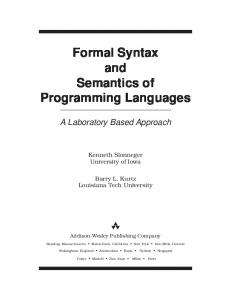
|| E(me) i G(chan gd, val tgen ) = |[ disc x , x = false | ∗(1tgen ; gd ! x) ]| D(chan gd, dc1 , dc2 , dr, val tout ) = |[ disc x | ∗(gd ? x ; (dc1 ! x [] dc2 ! x [] 1tout ; dr ! x)) ]| R(chan dr) = |[ disc x | ∗(dr ? x) ]| MA (chan cm1 , cm2 , me, val pt) = |[ disc x, y | ∗((cm1 ? x || cm2 ? y); 1pt; me ! x) ]| E(chan me) = |[ disc x | ∗(me ? x) ]| Every tgen time units (assuming tgen ≥ tout , see process D), a product is generated by generator G. A product is modeled by a boolean variable x that is initially false. The boolean indicates whether the product has done the second round in a manufacturing cell C. A product enters the manufacturing line via channel gd. The distributor tries to send a product either via channel dc1 or channel dc2 . In case this is not possible within tout time units, the product is rejected and sent to reject process R via channel dr (dc1 ! x [] dc2 ! x [] 1tout ; dr ! x). Process R consumes the rejected products (∗(dr ? x)). A manufacturing cell C, shown in Figure 4.2, consists of two machines (Mrw , M) and a N -place FIFO (first-in-first-out) buffer B.

in

Mrw

mb

B

bm

M

out

mm

Figure 4.2: Iconic model of a manufacturing cell C. The χ specification of the manufacturing cell is as follows: C(chan in, out, val pt min1, pt max1 , N, pt min2 , pt max2 ) |[ chan mb, bm, mm

35

| Mrw (in, mb, mm, pt min1 , ptmax1 ) || B(mb, bm, N) || M(bm, out, mm, ptmin2 , pt max2 ) ]| Products enter the cell via channel in. The routing of a product in the manufacturing cell is as follows: Mrw , B, M, Mrw , B, M. Products leave the manufacturing cell via channel out. The process definitions of the buffer and the machines are given by B(chan in, out, val N) = |[ disc x , xs = [ ] | ∗( len(xs) < N → in ? x ; xs := xs ++[x] [] len(xs) > 0 → out ! hd(xs); xs := tl(xs) ) ]| Mrw (chan in, out, mm, val ptmin , ptmax ) = |[ disc x, pt | ∗((in ? x [] mm ? x ; x := true); pt : pt ∈ [ptmin , ptmax ]; 1pt; out ! x) ]| M(chan in, out, mm, val ptmin , ptmax ) = |[ disc x, pt | ∗(in ? x ; pt : pt ∈ [ptmin , ptmax ]; 1pt; (x → out ! x [] ¬x → mm ! x)) ]| The buffer can store up to N products, which are stored in a list xs (len(xs) < N → in ? x ; xs := xs ++[x]), where [x] denotes a list with one element x, and ++ denotes list concatenation. The empty list is denoted by [ ]. If the buffer is not empty, the first product in the buffer can be sent to the machine via channel out (len(xs) > 0 → out ! hd(xs); xs := tl(xs)), where hd(xs) denotes the first element (head) of list xs, and tl(xs) denotes the remainder (tail) of list xs without its first element. Machine Mrw receives products from channels in and mm. A product received from mm is assigned the value true, which indicates that this product is processed by machine Mrw for the second time (in ? x [] mm ? x ; x := true). The machine has a processing time between ptmin and ptmax time units (pt : pt ∈ [ptmin , ptmax ]; 1pt). Processed products are sent via channel out to the buffer B. Machine M receives products via channel in, and processes them for pt time units. Depending on the value of product variable x, the product is sent either via channel mm to machine Mrw (x equals false) or it leaves the manufacturing cell via channel out (x equals true) (x → out ! x [] ¬x → mm ! x). After processing in one of the two manufacturing cells C, products are sent to machine MA . Machine MA waits to receive one product via channel cm1 , and one product via channel cm2 ,

36

Chapter 4. Discrete-event model of a manufacturing line

in a non-deterministic order (cm1 ? x || cm2 ? y). After processing these two products (1pt), the combination of them leaves the manufacturing line via channel out (out ! x). Process E consumes the processed products.

Chapter 5

Translating timed automata to timed Chi In this chapter, the timed automata model is translated to the timed χ formalism.

5.1 Definition of a timed automaton A timed automaton (based on [11]) consists of the following components: • A finite set of (real-valued) clocks X = {x1 , . . . , xn }, and a finite set Y = {y1 , . . . , ym } of variables. • A finite directed multi-graph (V, E), where V denotes a set of vertices (locations / control modes) and E denotes a set of edges (control switches). Vertex v0 ∈ V denotes the initial location. • A vertex labeling function inv that assigns an invariant to each location v ∈ V , and a vertex labeling function init that assigns an initialization predicate to the initial location v0 . Invariants and initialization predicates are predicates over variables and clocks. • Three edge labeling functions guard, reset, and assign that assign to each edge e ∈ E, a guard, clock resets, and assignments to variables, respectively. Guards are predicates over variables and clocks, and clock resets are of the form x := 0, where x denotes a clock. • A finite set 6 of events, and an edge labeling function event ∈ E → 6 that assigns an event to each edge e ∈ E.

37

38

Chapter 5. Translating timed automata to timed Chi

5.2 General translation scheme Consider a timed automaton with n clock variables (X = {x1 , . . . , xn }), m discrete variables (Y = {y1, . . . , ym }), k locations (V = {v1 , . . . , vk }), and initial location v1 , to be translated to a corresponding χ specification. The translation is defined as follows: h |[R { v1 7 → ¬(TC (inv(v1 ))) → ⊥ ([]e:e∈edges(v1 ) [TC (guard(e)) → TA (TR (reset(e)), TC (assign(e))) event(e)]; target(e) ) .. . , vk 7 → ¬(TC (inv(vk ))) → ⊥ ([]e:e∈edges(vk ) [TC (guard(e)) → TA (TR (reset(e)), TC (assign(e))) event(e)]; target(e) ) } | v1 ]| , R(init(v1 )) ∪ {time 7 → 0}, (∅, ∅) i The delay behavior in a vertex vi is restricted by means of its invariant. This restriction is translated to the process term ⊥, guarded with the negation of its invariant (¬(TC (inv(vi ))) → ⊥). Function TC replaces all clock variables x by expressions time − x. E.g. invariant TC (x ≤ 2) becomes time − x ≤ 2. Each outgoing edge is translated to a process term of the form [b → W : r la ; X ]. In this process term, the guard b is defined as TC (guard(e)). The label of the action predicate is defined as event(e), and the predicate r is defined as TA (TR (reset(e)), TC (assign(e))), where function TR replaces a clock reset x := 0 by x := time, and function TA combines clock resets and assignments into one action predicate. For example TA (x := time, y := 2) becomes {x, y} : x = time ∧ y = 2. Function R translates an init predicate x0 = c0 ∧ · · · ∧ xn = cn to a valuation {x0 7 → c0 , . . . , xn 7 → cn } . E.g. R(x = 1 ∧ y = 2) = {x 7 → 1, y 7 → 2}. In the translation scheme, the δ process term cannot be used instead of the inconsistent process term ⊥. Consider for instance a timed automaton with one clock variable x, one location v0 , function init(v0 ) = (x = 0) and function inv(v0 ) = (x < 1). This automaton can perform time transitions with duration t ∈ [0, 1). Using the translation scheme, the following χ process is obtained: h|[R v0 7 → ¬(time − x < 1) → ⊥ | v0 ]|, {x 7 → 0, time 7 → 0}, (∅, ∅)i. Like the timed automaton model, this process can perform time transitions of duration t ∈ [0, 1). Translating the timed automaton model to χ, using δ instead of ⊥, the following χ process is obtained: h|[R v0 7 → ¬(time − x < 1) → δ | v0 ]|, {x 7 → 0, time 7 → 0}, (∅, ∅)i. This process can perform time transitions of duration t ∈ [0, 1], including t = 1, and is therefore incorrect.

5.3. Example: a coffee vendor machine

39

5.3 Example: a coffee vendor machine 5.3.1 Timed automaton model of the coffee vendor machine After receiving a coin, modeled by means of action coin in the timed automaton model of Figure 5.1, the coffee machine allows the user to push a button (action button) within 5 time units. If the user pushes the button within this time interval, the machine produces the coffee after 2 to 4 time units (coffee). Otherwise, the machine refunds after 0.1 to 1 time units (refund).

x=0

s1

coin x := 0

x >2 coffee

x > 0.1 refund

s2 x ≤5

x 2 → ∅ : true coffee]; s1 , s4 7 → ¬(time − x ≤ 1) → ⊥ [] [time − x > 0.1 → ∅ : true refund]; s1 } | s1 ]| , {time 7 → 0, x 7 → 0, (∅, ∅) i

Chapter 6

Derivation of timed Chi from hybrid Chi In this chapter, the timed χ language is derived from the hybrid χ language defined in [17], such that hybrid χ is an operational conservative extension of timed χ. This derivation is divided into two main steps: 1) the syntax of hybrid χ is restricted (Section 6.1), 2) the continuous and algebraic variables are removed (Section 6.2).

6.1 The L1 language Let L0 (C, L) be the hybrid χ language, where C and L denote the set of continuous variables and the set of algebraic variables, respectively. Restricting the syntax of the L0 language leads to the L1 language. The syntactic restrictions are listed below: • remove delay predicate u, • remove jump enabling operator ι J + , • remove variable scope operators |[V σdx⊥ , {x}, {g} | p ]|, where {x} 6 = ∅ or {g} 6 = ∅. Therefore, the remaining variable scope operators in the L1 language are of the form |[V σdx⊥ , ∅, ∅ | p ]|. This results in the following syntax for the process terms p ∈ PL1 of the L1 language: PL1 ::= | | | |

W : r la | δ | ⊥ [P] | u y P | P ; P | b → P | P [] P P || P | h !! en | h ?? xn | ∂ A (P) | υH (P) X | |[V σ⊥ , ∅, ∅ ‘|’P ]| | |[H H0 ‘|’P ]| | |[R R ‘|’P ]| PextL1

41

Chapter 6. Derivation of timed Chi from hybrid Chi

42

PextL1 ::= | | |

skip | xn := en | xn : r | h ! en | h ? xn 1d (P) | 1d | ∗P | ∗b : P |[ disc sk , chan hm , i, L R ‘|’P ]| lp (xk , hm , en )

The deduction system of L1 , denoted by DL1 , consists of all deduction rules of the deduction system of L0 in which only syntax from L1 is used, i.e., the deduction rules defining atomic process terms and operators that are removed are omitted. Lemma 1 DL1 ⊂ DL0 .

Proof. Trivial

Lemma 2 If all syntax used in the conclusion of a deduction rule from DL0 is contained in L1 , then all syntax used in the hypothesis of this rule is also contained in L1 .

Proof. Trivial

Lemma 3 Let p and p0 be closed process terms from PL1 , σ, σ 0 be valuations, ξ, ξ 0 be extended valuations, (C, J, L , R) and (C 0 , J 0 , L 0 , R 0 ) be environments, a be an action, ρ be a trajectory, and t ∈ T . Then ξ,a,ξ 0

L0 (C, L) |H h p, σ, (C, J, L , R)i −−−→ h , σ 0 , (C 0 , J 0 , L 0 , R 0 )i

⇔

ξ,a,ξ 0

L1 (C, L) |H h p, σ, (C, J, L , R)i −−−→ h , σ 0 , (C 0 , J 0 , L 0 , R 0 )i, t,ρ

L0 (C, L) |H h p, σ, (C, J, L , R)i 7 −→ h p0 , σ 0 , (C 0 , J 0 , L 0 , R 0 )i t,ρ

0

0

0

0

0

⇔

0

L1 (C, L) |H h p, σ, (C, J, L , R)i 7 −→ h p , σ , (C , J , L , R )i, L0 (C, L) |H h p, σ, (C, J, L , R)i L1 (C, L) |H h p, σ, (C, J, L , R)i

ξ ξ

⇔ ,

ξ,a,ξ 0

where h p, σ, (C, J, L , R)i −−−→ h , σ 0 , (C 0 , J 0 , L 0 , R 0 )i is an abbreviation for ξ,a,ξ 0 X h p, σ, (C, J, L , R)i −−−→ h 0 , σ 0 , (C 0 , J 0 , L 0 , R 0 )i for some p0 . p Proof. The proof for the three statements of the lemma are very similar. Therefore, we only consider the second statement. Proof of left implication (⇐): We prove this lemma by induction on the depth of the proof of a time transition derived in L1 (C, L) and use case distinction on

6.2. The L2 language

43

the deduction rule applied last. If a time transition can be derived from DL1 , there exists a deduction rule from DL1 and a substitution such that this transition is obtained from applying the substitution to the deduction rule. Using Lemma 1, this deduction rule is also part of DL0 . By induction (Lemma 2 guarantees that the substituted hypotheses are also L1 (C, L)-terms) the substituted hypotheses of the deduction rule are also derivable in L0 (C, L). Therefore, using the same deduction rule and the same substitution, the transition can be derived in L0 (C, L) as well. Proof of right implication (⇒): The proof follows the same lines with the additional observation that due to Lemma 2, a proof of a transition between L1 (C, L)-terms will never use a deduction rule that is not also contained in DL1 .

6.2 The L2 language The L2 language is defined as L2 ≡ L1 (∅, ∅). The syntax of L2 remains unchanged w.r.t. L1 . The deduction system of L2 equals the deduction system DL1 , where all occurrences of C and L are replaced by ∅ (this substitution is also applied to the functions and 4). Furthermore, mathematical equalities of the form dom(ξ ) = dom(σ ) H⇒ ξσ = ξ , dom(ξ ∅∅ ) = ∅ H⇒ σ ∪ ξ ∅∅ = σ are used. Some free variables are renamed to other free variables for a more intuitive representation. After the substitution, all environments are of the form (∅, J, ∅, R). Since, there are no deduction rules which can modify the empty sets of the environment, this information is redundant. Hence, the environment is simplified to (J, R). To illustrate how DL2 is derived from DL1 , the derivation is shown below for function 4, function and the deduction rule of the action transition of the action predicate in DL2 . The other derivations can be found in Appendix A. Substitution [∅, ∅/C, L] on function definition 4, 4(σ, C, J, L) = {ξ | dom(ξ ) = dom(σ ) ∪ C˙ ∪ L , ∀x∈dom(σ )\ J ξ(x) = σ (x)} results in the following definition: 4(σ, J ) = {σ 0 | dom(σ 0 ) = dom(σ ), ∀x∈dom(σ )\ J σ 0 (x) = σ (x)}, using C = ∅ H⇒ C˙ = ∅, and bound variable ξ is substituted by bound variable σ 0 . The signature of the function is simplified to 4 ∈ (6 × P(V )) → P(6). All occurrences of function in the deduction rules of DL2 are of the form (σ, C, L , u, t) (or in abbreviated notation σEt ), where u ≡ true. Therefore, in the function definition for true can be substituted for u. Substitution [∅, ∅, true/C, L , u] on function definition ,


44

(σ, C, L , u, t) = {ρ | ρ ∈ [0, t] 7 → ((dom(σ ) ∪ C˙ ∪ L) → 3) ,t ≥0 , ∀s ∈ [0, t] : ρ(s) |H u , ∀x ∈ C˙ ∪ L : ρ ↓ x is a bounded function that is absolutely continuous except for a finite number of points , ∀x ∈ dom(σ ) \ ({time} ∪ C) : ρ ↓ x is a constant function , ∀x ∈ C : ρ ↓ x is an absolutely continuous function , ∀x ∈ dom(σ ) : (ρ  ↓ x)(0) = σ (x) Rs ˙ 0 )ds 0  (ρ ↓ x)(s) = (ρ ↓ x)(0) + 0 (ρ ↓ x)(s , ∀s ∈ [0, t], x ∈ C : ρ ↓ x is differentiable in s ⇒  (ρ ↓ x)(s) ˙ = ( dtd (ρ ↓ x))(s) , ∀s ∈ [0, t] : ρ(s)(time) = σ (time) + s } results in the following definition: (σ, t) = {ρ | ρ ∈ [0, t] 7 → ((dom(σ )) → 3) ,t ≥0 , ∀x ∈ dom(σ ) \ {time} : ρ ↓ x is a constant function , ∀x ∈ dom(σ ) : (ρ ↓ x)(0) = σ (x) , ∀s ∈ [0, t] : ρ(s)(time) = σ (time) + s }

using C = ∅ H⇒ C˙ = ∅. The signature of the function is simplified to ∈ 6 × T → P(T 7 → 6). Substitution of [∅, ∅/C, L] on the deduction rule for the action transition of the action predicate, ˙

ξ = σ ∪ ξ C L , ξ 0 ∈ 4(σ, C, J ∪ W, L), ξ − ∪ ξ 0 |H r ξ , la , ξ 0 (C, J, L , R) hW : r la , σ i −−−−→ hX, ξσ0 i results in the following deduction rule: σ 0 ∈ 4(σ, J ∪ W ), σ − ∪ σ 0 |H r L2 -1 σ , la , σ 0 (J, R) hW : r la , σ i −−−−−→ hX, σ 0 i ˙

using dom(ξ C L ) = ∅ H⇒ ξ = σ , dom(ξ 0 ) = dom(σ ) H⇒ ξσ0 = ξ 0 , and free variables ξ 0 and ξ − are substituted by σ 0 and σ − , respectively.

6.3. Relating L0 (∅, ∅) and L2

45

Lemma 4 Let p and p0 be closed process terms from PL2 , σ, σ 0 be valuations, ξ, ξ 0 be extended valuations, J and J 0 be sets of jumping variables, R and R 0 be recursion definitions, a be an action, ρ be a trajectory, and t ∈ T . Then ξ,a,ξ 0

L1 (∅, ∅) |H h p, σ, (∅, J, ∅, R)i −−−→ h , σ 0 , (∅, J 0 , ∅, R 0 )i ⇔ ξ,a,ξ 0

L2 |H h p, σ, (J, R)i −−−→ h , σ 0 , (J 0 , R 0 )i t,ρ

L1 (∅, ∅) |H h p, σ, (∅, J, ∅, R)i 7 −→ h p0 , σ 0 , (∅, J 0 , ∅, R 0 )i ⇔ t,ρ

L2 |H h p, σ, (J, R)i 7 −→ h p0 , σ 0 , (J 0 , R 0 )i L1 (∅, ∅) |H h p, σ, (∅, J, ∅, R)i L2 |H h p, σ, (J, R)i

ξ

ξ

⇔

,

ξ,a,ξ 0

h p, σ, (∅, J, ∅, R)i −−−→ h , σ 0 , (∅, J 0 , ∅, R 0 )i is an abbreviation for ξ,a,ξ 0 ξ,a,ξ 0 X h p, σ, (∅, J, ∅, R)i −−−→ h 0 , σ 0 , (∅, J 0 , ∅, R 0 )i for some p0 , and h p, σ, (J, R)i −−−→ p ξ,a,ξ 0 X h , σ 0 , (J 0 , R 0 )i is an abbreviation for h p, σ, (J, R)i −−−→ h 0 , σ 0 , (J 0 , R 0 )i for some p0 . p where

Proof. This proof follows the same lines as the proof of Lemma 3. There are two important differences. The first difference is that the deduction rules of L1 (∅, ∅) and the deduction rules of L2 are syntactically different. Nevertheless, by construction of the deduction system of L2 , there is a one-to-one mapping between these sets of deduction rules that explains precisely how the application of a deduction rules from one of these languages has to be mimicked by the application of a deduction rule from the other language. The second difference is that, due to the renaming of some variables in the original deduction rule, the substitutions that are used in deriving in the two deduction systems are not identical anymore. Again, by construction, i.e. using the mathematical identities as defined in this section and in Appendix A, also here it is clear how a substitution used for deriving a transition in L1 (∅, ∅) can be transformed into a substitution used for deriving the same transition in L2 , and vice versa.

6.3 Relating L0 (∅, ∅) and L2 From Lemma 3 and 4 we obtain the following relation between L0 (∅, ∅) and L2 : Corrolary 1 Let p and p0 be closed process terms from PL2 , σ, σ 0 be valuations, ξ, ξ 0 be extended valuations, J and J 0 be sets of jumping variables, R and R 0 be recursion definitions,


46

a be an action, ρ be a trajectory, and t ∈ T . Then ξ,a,ξ 0

L0 (∅, ∅) |H h p, σ, (∅, J, ∅, R)i −−−→ h , σ 0 , (∅, J 0 , ∅, R 0 )i ⇔ ξ,a,ξ 0

L2 |H h p, σ, (J, R)i −−−→ h , σ 0 , (J 0 , R 0 )i t,ρ

L0 (∅, ∅) |H h p, σ, (∅, J, ∅, R)i 7 −→ h p0 , σ 0 , (∅, J 0 , ∅, R 0 )i ⇔ t,ρ

L2 |H h p, σ, (J, R)i 7 −→ h p0 , σ 0 , (J 0 , R 0 )i L0 (∅, ∅) |H h p, σ, (∅, J, ∅, R)i L2 |H h p, σ, (J, R)i

ξ

ξ

⇔

,

ξ,a,ξ 0

h p, σ, (∅, J, ∅, R)i −−−→ h , σ 0 , (∅, J 0 , ∅, R 0 )i ξ,a,ξ 0 X h p, σ, (∅, J, ∅, R)i −−−→ h 0 , σ 0 , (∅, J 0 , ∅, R 0 )i for some p0 . p where

is

an

abbreviation

for

6.4 Relating L2 and timed Chi Let h¯ be a bijective mapping that maps the process terms of the L2 language to the process terms of the timed χ language. It is defined as h¯ (|[V σ⊥ , ∅, ∅ ‘|’P ]|) = |[V σ⊥ ‘|’h¯ (P) ]|, and distributes over all other operators. Lemma 5 Let p and p0 be closed process terms from the L2 language, σ, σ 0 , ξ, ξ 0 be valuations, J and J 0 be sets of jumping variables, R and R 0 be recursion definitions, a be an action, ρ be a trajectory, and t ∈ T . Then ξ,a,ξ 0

L2 |H h p, σ, (J, R)i −−−→ h , σ 0 , (J 0 , R 0 )i ξ,a,ξ 0

0

0

⇔ 0

timed χ |H hh¯ ( p), σ, (J, R)i −−−→ h , σ , (J , R )i t,ρ L2 |H h p, σ, (J, R)i 7 −→ h p0 , σ 0 , (J 0 , R 0 )i

⇔

t,ρ

timed χ |H hh¯ ( p), σ, (J, R)i 7 −→ hh¯ ( p0 ), σ 0 , (J 0 , R 0 )i L2 |H h p, σ, (J, R)i

ξ

timed χ |H hh¯ ( p), σ, (J, R)i ξ,a,ξ 0

⇔ ξ

, ξ,a,ξ 0

where h p, σ, (J, R)i −−−→ h , σ 0 , (J 0 , R 0 )i is an abbreviation for h p, σ, (J, R)i −−−→ ξ,a,ξ 0 X h 0 , σ 0 , (J 0 , R 0 )i for some p0 , and hh¯ ( p), σ, (J, R)i −−−→ h , σ 0 , (J 0 , R 0 )i is an abbreviation p ξ,a,ξ 0 X , σ 0 , (J 0 , R 0 )i for some p0 . for hh¯ ( p), σ, (J, R)i −−−→ h h( ¯ p0 ) Proof. Trivial

Chapter 7

Validation of the semantics First we consider the well-definedness of the semantics in Section 7.1. Then, in Section 7.2, some properties of the Chi semantics are given. In Section 7.3, a notion of equivalence is defined, called stateless bisimilarity [12], which is similar to the well-known notion of bisimilarity [15, 10]. It is also shown that this relation is an equivalence and a congruence for all χ operators. Some useful properties of closed χ process terms are given in Section 7.4. Many of these properties express intuitions about the meaning of the χ operators such as the commutativity and associativity of the alternative composition and the parallel composition operator. Other properties are introduced for the purpose of simplifying χ models. Both the examples treated in the previous section and the properties treated in this section add to the level of confidence one has with respect to the ‘correctness’ of the semantics.

7.1 Well-definedness of the semantics In the term deduction system negative hypotheses are used in Rule 34 of the urgency communication operator. As a consequence it is not obvious at first sight whether the term deduction system defines a unique transition system for each closed process term. Well-definedness of the term deduction system can be obtained by providing a stratification [2]. The mapping that associates with every positive action transition and positive consistency predicate the value 0 and with every positive time transition the value 1, turns out to be a stratification.

7.2 Properties of the semantics In this section, some useful properties about the semantics of χ are introduced that can be applied in the remainder of the report (especially in the proofs of the properties in Section 7.4). With the current set of deduction rules for the semantics of χ, the left-hand and right-hand valuation are always the same as the initial and resulting valuation of an action transition, re-

47

Chapter 7. Validation of the semantics

48

spectively. A similar reasoning applies to the first and last valuation of a trajectory on a time transition and the initial and resulting valuation, respectively. Also note that the environment is never changed in a transition, and that the valuation on the consistency transition is the same as the initial valuation. The following lemma captures these facts. Lemma 6 Let p and p0 be closed process terms, σ, σ 0 , ξ, ξ 0 be valuations, E and E 0 be environments, a be an action, ρ be a trajectory, and t ∈ T . Then ξ,a,ξ 0

h p, σ, Ei −−−→ h , σ 0 , E 0 i ⇒ dom(σ ) = dom(σ 0 ) ∧ ξ = σ ∧ ξ 0 = σ 0 ∧E = E 0 , t,ρ

h p, σ, Ei 7 −→ h p0 , σ 0 , E 0 i ⇒ dom(ρ) = [0, t] ∧ ρ(0) = σ ∧ ρ(t) = σ 0 ∧E = E 0 , h p, σ, Ei

ξ

⇒ ξ = σ.

ξ,a,ξ 0

ξ,a,ξ 0

where h p, σ, Ei −−−→ h , σ 0 , E 0 i is an abbreviation for h p, σ, Ei −−−→ h

X 0 0 , σ , E i for some p0

p0 .

Proof. See Lemma 5, Corollary 1, and [17, Lemma 1].

If a χ process can perform action or time transitions, the process is consistent. Lemma 7 Let p and p0 be closed process terms, σ, σ 0 , ξ, ξ 0 be valuations, E and E 0 be environments, and a be an action. Then ξ,a,ξ 0

h p, σ, Ei −−−→

⇒ h p, σ, Ei

ξ

, ξ,a,ξ 0

ξ,a,ξ 0

where h p, σ, Ei −−−→ is an abbreviation for ∃ p0 ,σ 0 ,E 0 h p, σ, Ei −−−→ h

X 0 0 , σ , E i. p0


Lemma 8 Let p and p0 be closed process terms, σ and σ 0 be valuations, E and E 0 be environments, t ∈ T , and ρ be a trajectory. Then, t,ρ

h p, σ, Ei 7 −→ ⇒ h p, σ, Ei t,ρ

ρ(0)

,

t,ρ

where h p, σ, Ei 7 −→ is an abbreviation for ∃ p0 ,σ 0 ,E 0 h p, σ, Ei 7 −→ h p0 , σ 0 , E 0 i.

7.3. Stateless bisimilarity

49


The following lemma shows that any variation in the set of jumping variables in the environment of a consistent χ process has no effect on the consistency transition. Lemma 9 Let p be a closed process term, σ, ξ be a valuations, J, W be sets of variables such that J and W ⊆ dom(σ ) \ {time}, and R be a recursion definition. Then h p, σ, (J, R)i

ξ

⇔ h p, σ, (J ∪ W, R)i


ξ

.

7.3 Stateless bisimilarity Two closed χ process terms are considered equivalent if they have the same behavior (in the bisimulation sense) in case both are considered from the same initial valuation of model variables and the same environment. We also assume that the initial valuation contains at least the free occurrences of variables in the two closed χ process terms being equivalent. Definition 1 (Stateless bisimilarity) A stateless bisimulation relation on closed process terms is a relation R ⊆ P × P such that ∀( p, q) ∈ R, the following holds:

ξ,a,ξ 0

1. ∀σ, E, ξ, a, ξ 0 , σ 0 , E 0 : h p, σ, Ei −−−→ hX, σ 0 , E 0 i ξ,a,ξ 0

⇔ hq, σ, Ei −−−→ hX, σ 0 , E 0 i, ξ,a,ξ 0

2. ∀σ, E, ξ, a, ξ 0 , p0 , σ 0 , E 0 : h p, σ, Ei −−−→ h p0 , σ 0 , E 0 i ξ,a,ξ 0

⇒ ∃q 0 : hq, σ, Ei −−−→ hq 0 , σ 0 , E 0 i ∧ ( p0 , q 0 ) ∈ R, ξ,a,ξ 0

3. ∀σ, E, ξ, a, ξ 0 , q 0 , σ 0 , E 0 : hq, σ, Ei −−−→ hq 0 , σ 0 , E 0 i ξ,a,ξ 0

⇒ ∃ p0 : h p, σ, Ei −−−→ h p0 , σ 0 , E 0 i ∧ ( p0 , q 0 ) ∈ R, t,ρ

4. ∀σ, E, t, ρ, p0 , σ 0 , E 0 : h p, σ, Ei 7 −→ h p0 , σ 0 , E 0 i t,ρ ⇒ ∃q 0 : hq, σ, Ei 7 −→ hq 0 , σ 0 , E 0 i ∧ ( p0 , q 0 ) ∈ R, t,ρ

5. ∀σ, E, t, ρ, q 0 , σ 0 , E 0 : hq, σ, Ei 7 −→ hq 0 , σ 0 , E 0 i t,ρ ⇒ ∃ p0 : h p, σ, Ei 7 −→ h p0 , σ 0 , E 0 i ∧ ( p0 , q 0 ) ∈ R,


50

6. ∀σ, E, ξ : h p, σ, Ei

ξ

⇔ hq, σ, Ei

ξ

. t

Two closed process terms p and q are stateless bisimilar, denoted by p ↔ q, if there exists a stateless bisimulation relation R such that ( p, q) ∈ R. Note that in the above definition of stateless bisimilarity it is possible that the left-hand and right-hand valuation of model variables, as displayed on an action transition, are different from the respective valuations of model variables of the state before performing the action transition and the state reached by performing the action transition. Similarly, the valuation of model variables before and after a time transition can be different from the initial and end-point of a trajectory, respectively. As a consequence of Lemma 6, the definition of stateless bisimilarity can be simplified considerably. Yet, with in mind future extensions of the χ language, it might well be the case that these properties of the semantics are lost. Since we would prefer not to redo all the coming proofs (in such a future), this presentation was chosen. Stateless bisimilarity is proved to be a congruence with respect to all χ operators. As a consequence, algebraic reasoning is facilitated, since it is allowed to replace equals by equals in any context. Theorem 1 (Congruence) Stateless bisimilarity is a congruence with respect to all χ operators. Proof. The deduction rules of the χ language, satisfy the process-tyft format of [12]. Therefore, stateless bisimilarity is a congruence.

The hybrid χ language without continuous variables and algebraic variables, denoted by L0 (∅, ∅) (see Chapter 6), is an operational conservative extension of the timed χ language, i.e., for closed timed χ-terms, any equality and only equalities that can be derived in timed χ can also be derived in L0 (∅, ∅). Lemma 10 Let p and q be closed process terms from timed χ. Then L0 (∅, ∅) |H h¯ −1 ( p) ↔ h¯ −1 (q)

⇔

t

timed χ |H p ↔ q.

Proof. This follows immediately from the definition of h¯ as described in Section 6.4, Lemma t 5, Corollary 1, and the definitions of ↔ (see [17]) and ↔ (see Definition 1).

7.4. Properties of the Chi operators

51

7.4 Properties of the Chi operators In this section, some properties of the operators of χ that hold with respect to stateless bisimilarity are discussed. Most of these correspond well with our intuitions, and hence this can be considered as an additional validation of the semantics. It is not our intention to provide a complete list of such properties (complete in the sense that every equivalence between closed process terms is derivable from those properties). For the proofs of the properties, we refer to Lemma 10 and the proofs of the corresponding properties in [17]. Proposition 1 (Signal emission operator) The following properties hold for all closed process terms p ∈ P and predicates u, u 0 : true y p false y p u y (u 0 y p)

↔ ↔ ↔

p ⊥ (u ∧ u 0 ) y p

If a true predicate is emitted, the process term is simply executed. If falsity holds initially, the process term is inconsistent. A concatenation of signal emissions leads to a signal emission with conjunction of predicates. Proposition 2 (Alternative composition) The following properties hold for all closed process terms p, q, r ∈ P: p [] p ↔ p p [] q ↔ q [] p ( p [] q) [] r ↔ p [] (q [] r) The alternative composition is idempotent, commutative and associative. The property p [] δ ↔ p does not hold. Consider, for example p = false → skip. Then p [] δ cannot perform any time transitions, while p can perform arbitrary time transitions. Property p [] δ ↔ δ does not hold either. Consider, for example p = skip. Then p [] δ can perform a τ transition, while δ cannot. Proposition 3 (Guard operator) The following properties hold for all closed process terms p ∈ P and guard b: true → p ↔ p b → ( p [] q) ↔ b → p [] b → q If a process term is guarded by a true predicate, the process term is simply executed. The guard distributes over the alternative composition operator.


52

Proposition 4 (Sequential composition) The following properties hold for all closed process terms p, q, r ∈ P and guard b: δ; p ( p; q); r ( p [] q); r b → ( p; q)

↔ ↔ ↔ ↔

δ p; (q ; r) p; r [] q ; r (b → p); q

A deadlock process term followed by some other process terms is equivalent to the deadlock process term itself since the deadlock process term does not terminate successfully, i.e., deadlock is a left-zero element for sequential composition. Sequential composition is associative and alternative composition distributes over sequential composition from the left. A guard distributes to the left argument of a sequential composition. Proposition 5 (Parallel composition) The following properties hold for all closed process terms p, q, r ∈ P : p || q ↔ q || p ( p || q) || r ↔ p || (q || r) Parallel composition is commutative and associative. Proposition 6 (Action encapsulation operator) The following properties hold for all closed process terms p ∈ P, and sets of actions A, A0 : ∂∅ ( p) ∂A (∂A0 ( p))

↔ ↔

p ∂A∪A0 ( p)

If there are no actions to be encapsulated, the application of the action encapsulation operator to a process term p has no effect. Multiple applications of the action encapsulation operator are equivalent to a single application where all the actions to be encapsulated are combined using union of sets of actions. Proposition 7 (Inconsistent process) The following terms p ∈ P and predicate u: uy⊥ ↔ p [] ⊥ ↔ p || ⊥ ↔ ∂A (⊥) ↔ ⊥; p ↔ skip; ⊥ ↔

properties hold for all closed process ⊥ ⊥ ⊥ ⊥ ⊥ δ

The inconsistent process term is a zero element for signal emission operator, alternative composition, parallel composition and action encapsulation operator. It is also a left-zero element for sequential composition. Going on as ⊥ after performing an action transition, for example skip, is impossible.

Bibliography [1] J. Baeten and J. Bergstra. Process algebra with propositional signals. Theoretical Computer Science, 177(2):381–405, 1997. [2] J. Baeten and C. Verhoef. Concrete process algebra. In S. Abramsky, D. Gabbay, and T. Maibaum, editors, Handbook of Logic in Computer Science, volume 4 (Semantic Modelling), pages 149–268. Oxford University Press, 1995. [3] J. A. Bergstra and C. A. Middelburg. Process algebra for hybrid systems. Technical Report CS-Report 03-06, Eindhoven University of Technology, Department of Computer Science, The Netherlands, 2003. [4] V. Bos and J. J. T. Kleijn. Automatic verification of a manufacturing system. Robotics and Computer Integrated Manufacturing, 17(3):185–198, 2000. [5] V. Bos and J. J. T. Kleijn. Formal Specification and Analysis of Industrial Systems. PhD thesis, Eindhoven University of Technology, 2002. [6] P. J. L. Cuijpers, M. A. Reniers, and W. P. M. H. Heemels. Hybrid transition systems. Technical Report CS-Report 02-12, Eindhoven University of Technology, Department of Computer Science, The Netherlands, 2002. [7] G. Fábián. A Language and Simulator for Hybrid Systems. PhD thesis, Eindhoven University of Technology, 1999. [8] K. G. Larsen, P. Pettersson, and W. Yi. U PPAAL in a Nutshell. Int. Journal on Software Tools for Technology Transfer, 1(1–2):134–152, 1997. [9] N. Lynch, R. Segala, and F. Vaandrager. Hybrid I/O automata. Inf. Comput., 185(1):105– 157, 2003. [10] R. Milner. A Calculus of Communicating Systems, volume 92 of LNCS. Springer, 1980. [11] M. Möller. Structure and Hierarchy in Real-Time Systems. PhD thesis, University of Aarhus, 2002. [12] M. Mousavi, M. Reniers, and J. F. Groote. Congruence for SOS with data. In Proceedings of Nineteenth Annual IEEE Symposium on Logic in Computer Science (LICS’04), pages 302–313, Turku, Finland, 2004. IEEE Computer Society Press.

53

54

Bibliography

[13] G. Naumoski and W. Alberts. A Discrete-Event Simulator for Systems Engineering. PhD thesis, Eindhoven University of Technology, 1998. [14] X. Nicollin and J. Sifakis. The algebra of timed processes, ATP: Theory and application. Information and Computation, 114:131–178, 1994. [15] D. Park. Concurrency and automata on infinite sequences. In P. Deussen, editor, Proceedings 5t h GI Conference, volume 104 of LNCS, pages 167–183. Springer, 1981. [16] G. D. Plotkin. A structural approach to operational semantics. Technical Report DIAMI FN-19, Computer Science Department, Aarhus University, 1981. [17] D. A. van Beek, K. L. Man, M. A. Reniers, J. E. Rooda, and R. R. H. Schiffelers. Syntax and consistent equation semantics of hybrid Chi. Technical Report CS-Report 04-37, Eindhoven University of Technology, Department of Computer Science, The Netherlands, 2004. [18] D. A. van Beek and J. E. Rooda. Languages and applications in hybrid modelling and simulation: Positioning of Chi. Control Engineering Practice, 8(1):81–91, 2000. [19] D. A. van Beek, A. van den Ham, and J. E. Rooda. Modelling and control of process industry batch production systems. In 15th Triennial World Congress of the International Federation of Automatic Control, Barcelona, 2002. CD-ROM.

Appendix A

Derivation of DL2 from DL1 This appendix shows the derivation of the deduction rules of DL2 from DL1 , as described in Section 6.2. Sections A.1 and A.2 show the derivation for the atomic process terms and the operators, respectively. The deduction rules from DL2 which are not shown in these sections are syntactically equivalent to their corresponding deduction rules in DL1 . Deduction rules with a label of the form L2 -n, where n denotes the number of the deduction rule, are from DL2 . The other deduction rules are from DL1 .

A.1

Derivation for atomic process terms

Action predicate ˙

ξ = σ ∪ ξ C L , ξ 0 ∈ 4(σ, C, J ∪ W, L), ξ − ∪ ξ 0 |H r 1 ξ , la , ξ 0 (C, J, L , R) hW : r la , σ i −−−−→ hX, ξσ0 i

σ 0 ∈ 4(σ, J ∪ W ), σ − ∪ σ 0 |H r L2 -1 σ , la , σ 0 0 (J, R) hW : r la , σ i −−−−−→ hX, σ i • Environment (C, J, L , R) is simplified to (J, R), ˙

• dom(ξ C L ) = ∅ H⇒ ξ = σ , • dom(ξ 0 ) = dom(σ ) H⇒ ξσ0 = ξ 0 , • free variables ξ 0 and ξ − are renamed to σ 0 and σ − , respectively, • for function 4 see Section 6.2.

55

Appendix A. Derivation of DL2 from DL1

56

(C, J, L , R) hW : r la , σ i

E hW : r la , σ i

σ

σ ∪ξ C˙ L

2

L2 -2

• Environment (C, J, L , R) is simplified to (J, R), and denoted by E, ˙

˙

• dom(ξ C L ) = ∅ H⇒ σ ∪ ξ C L = σ . Send and receive ˙

ξ = σ ∪ ξ C L , ξ 0 ∈ 4(σ, C, J, L) 3 ξ , isa(h,[ξ(en )]) , ξ 0 0 (C, J, L , R) hh !! en , σ i −−−−−−−−−−→ hX, ξσ i

σ 0 ∈ 4(σ, J ) L2 -3 σ , isa(h,[σ (en )]) , σ 0 (J, R) hh !! en , σ i −−−−−−−−−−−→ hX, σ 0 i • Environment (C, J, L , R) is simplified to (J, R), ˙

• dom(ξ C L ) = ∅ H⇒ ξ = σ , • dom(ξ 0 ) = dom(σ ) H⇒ ξσ0 = ξ 0 , • free variable ξ 0 is renamed to σ 0 , • for function 4 see Section 6.2.

˙

ξ = σ ∪ ξ C L , ξ 0 ∈ 4(σ, C, J ∪ {xn }, L), ξ 0 (xn ) = cn 4 ξ , ira(h,[cn ],{xn }) , ξ 0 (C, J, L , R) hh ?? xn , σ i −−−−−−−−−−−→ hX, ξσ0 i

σ 0 ∈ 4(σ, J ∪ {xn }), σ 0 (xn ) = cn L2 -4 σ , ira(h,[cn ],{xn }) , σ 0 0 (J, R) hh ?? xn , σ i −−−−−−−−−−−−→ hX, σ i • Environment (C, J, L , R) is simplified to (J, R), ˙

• dom(ξ C L ) = ∅ H⇒ ξ = σ , • dom(ξ 0 ) = dom(σ ) H⇒ ξσ0 = ξ 0 ,

A.1. Derivation for atomic process terms

57

• free variable ξ 0 is renamed to σ 0 , • for function 4 see Section 6.2.

(C, J, L , R) hh !! en , σ i

E hh !! en , σ i

σ

σ ∪ξ C˙ L

5

L2 -5


˙

• dom(ξ C L ) = ∅ H⇒ σ ∪ ξ C L = σ .

(C, J, L , R) hh ?? xn , σ i E hh ?? xn , σ i

σ

σ ∪ξ C˙ L

6

L2 -6


˙

• dom(ξ C L ) = ∅ H⇒ σ ∪ ξ C L = σ . Consistent deadlock

(C, J, L , R) hδ, σ i

E hδ, σ i

σ

σ ∪ξ C˙ L

7

L2 -7


˙

• dom(ξ C L ) = ∅ H⇒ σ ∪ ξ C L = σ .


58

A.2

Derivation for operators

Delay enabling operator ρ ∈ σEt

E

9

t,ρ

h[ p], σ i 7 −→ h[ p], ρσ (t)i ρ ∈ (σ, t)

E

L2 -9

t,ρ

h[ p], σ i 7 −→ h[ p], ρ(t)i • dom(range(ρ)) = dom(σ ) H⇒ ρσ = ρ, • for function see Section 6.2.

(C, J, L , R) h[ p], σ i

E h[ p], σ i

σ

σ ∪ξ C˙ L

10

L2 -10


˙

• dom(ξ C L ) = ∅ H⇒ σ ∪ ξ C L = σ . Guard operator ρ ∈ σEt , ∀s∈(0,t ) ρ(s) |H ¬b, 0,ρ {0}

ρ(0) |H b ⇒ h p, σ i 7 −→ h p0 , σ 0 i, E

ρ(t) |H b ⇒ h p, ρσ (t)i

ρ(t )

t,ρ

20

hb → p, σ i 7 −→ hb → p, ρσ (t)i

ρ ∈ (σ, t), ∀s∈(0,t ) ρ(s) |H ¬b, 0,ρ {0}

ρ(0) |H b ⇒ h p, σ i 7 −→ h p0 , σ 0 i E

ρ(t) |H b ⇒ h p, ρ(t)i t,ρ

ρ(t )

hb → p, σ i 7 −→ hb → p, ρ(t)i • dom(range(ρ)) = dom(σ ) H⇒ ρσ = ρ, • for function see Section 6.2.

L2 -20

A.2. Derivation for operators

59

˙

σ ∪ ξ C L |H ¬b (C, J, L , R) hb → p, σ i

σ |H ¬b E hb → p, σ i

σ

σ ∪ξ C˙ L

22

L2 -22


˙

• dom(ξ C L ) = ∅ H⇒ σ ∪ ξ C L = σ . Parallel composition operator *X + p0 0 (C, J ∪ W, L , R) h p, σ i −−−−−−→ ,σ , X p0 *X + ξ,ira(h,cs,W ),ξ 0 X 0 (C, J, L , R) hq, σ i −−−−−−−−→ ,σ q0 q0 ξ,isa(h,cs),ξ 0

ξ,ca(h,cs),ξ 0

(C, J, L , R) h p || q, σ i −−−−−−→

ξ,ca(h,cs),ξ 0

hq || p, σ i −−−−−−→

*

*

X + p0 0 ,σ , q0 p0 || q 0 +

X p0 ,σ0 q0 q 0 || p0

26


60

*X + p0 0 (J ∪ W, R) h p, σ i −−−−−−→ ,σ , X p0 + *X ξ,ira(h,cs,W ),ξ 0 X 0 ,σ (J, R) hq, σ i −−−−−−−−→ q0 q0 ξ,isa(h,cs),ξ 0

X + ξ,ca(h,cs),ξ 0 p0 0 ,σ , (J, R) h p || q, σ i −−−−−−→ q0 p0 || q 0 * X + ξ,ca(h,cs),ξ 0 p0 hq || p, σ i −−−−−−→ ,σ0 q0 q 0 || p0 *

• Environment (C, J ∪ W, L , R) is simplified to (J ∪ W, R), • environment (C, J, L , R) is simplified to (J, R). Recursion variable α

hR(X ), σ i − →h (C, J, L , R) α

hX, σ i − →h

α

hR(X ), σ i − →h (J, R)

X 0 ,σ i p0

X 0 ,σ i p0

X 0 ,σ i p0

X hX, σ i − → h 0 , σ 0i p

36

L2 -36

α

• Environment (C, J, L , R) is simplified to (J, R). t,ρ

(C, J, L , R)

hR(X ), σ i 7 −→ h p0 , σ 0 i t,ρ

37

hX, σ i 7 −→ h p0 , σ 0 i

t,ρ

(J, R)

hR(X ), σ i 7 −→ h p0 , σ 0 i t,ρ

hX, σ i 7 −→ h p0 , σ 0 i

L2 -37

L2 -26


61

• Environment (C, J, L , R) is simplified to (J, R).

(C, J, L , R)


(J, R)


ξ

ξ

38

ξ

ξ

L2 -38

• Environment (C, J, L , R) is simplified to (J, R). Variable scope operator ξ,a,ξ 0

(C ∪ {x00 }, J, L ∪ {g00 }, R) h p[d0 , x00 , g00 /d, x0 , g0 ], σ ∪ σd0 x00 i −−−→ h

X 0 ,σ i p0

κσ C˙ L (ξ,a,ξ 0 )

39

(C, J, L , R) h|[V σdx0⊥ , {x0 }, {g0 } | p ]|, σ i −−−−−−→ h

X ,σ0 i |[V (σ 0 {d0 , x00 })[d, x0 /d0 , x00 ], {x0 }, {g0 } | p0 [d, x0 , g0 /d0 , x00 , g00 ] ]| σ

ξ,a,ξ 0

h p[d0 /d], σ ∪ σd0 i −−−→ h E

X 0 ,σ i p0

X h|[V σd⊥ , ∅, ∅ | p ]|, σ i −−−−−→ h ,σ0 i 0 0 |[V (σ {d })[d/d0 ], ∅, ∅ | p0 [d/d0 ] ]| σ κσ (ξ,a,ξ 0 )

L2 -39

• {x0 } = ∅ H⇒ {x00 } = ∅, • {g0 } = ∅ H⇒ {g00 } = ∅, • {x00 } = ∅ ∧ {g00 } = ∅ H⇒ (C ∪ {x00 }, J, L ∪ {g00 }, R) = (C, J, L , R), • environment (C, J, L , R) is simplified to (J, R), and denoted by E, • notation σdx0⊥ is simplified to σd⊥ , which is defined as σd⊥ ∈ {d} 7 → (3 ∪ ⊥). Notation σd0 x00 is simplified to σd0 , which is defined as σd0 ∈ {d0 } 7 → (3), • substitution p[d0 , x00 , g00 /d, x0 , g0 ] is simplified to p[d, x0 , g0 /d0 , x00 , g00 ] is simplified to p[d/d0 ],

p[d0 /d],

and substitution


62

• substitution [∅, ∅/C, L] on function definition κ for arbitrary receive actions ira(h, cs, W ): κσ C˙ L (ξ, ira(h, cs, W ), ξ 0 ) = ξσ C˙ L , ira(h, cs, W ∩ (dom(σ ) ∪ L)), ξσ0 C˙ L , and for all other actions: κσ C˙ L (ξ, a, ξ 0 ) = ξσ C˙ L , a, ξσ0 C˙ L , result in the following definition for arbitrary receive actions ira(h, cs, W ): κσ (ξ, ira(h, cs, W ), ξ 0 ) = ξσ , ira(h, cs, W ∩ dom(σ )), ξσ0 , and for all other actions: κσ (ξ, a, ξ 0 ) = ξσ , a, ξσ0 , where valuations ξσ and ξσ0 denote ξ dom(σ ) and ξ 0 dom(σ ), respectively. The signature of function κ is simplified to κ ∈ 6 × 6 × A × 6 → 6 × A × 6. t,ρ

(C ∪ {x00 }, J, L ∪ {g00 }, R) h p[d0 , x00 , g00 /d, x0 , g0 ], σ ∪ σd0 x00 i 7 −→ h p0 , σ 0 i t,ρσ C˙ L

40

(C, J, L , R) h|[V σdx0⊥ , {x0 }, {g0 } | p ]|, σ i 7 −→

h|[V (σ 0 {d0 , x00 })[d, x0 /d0 , x00 ], {x0 }, {g0 } | p0 [d, x0 , g0 /d0 , x00 , g00 ] ]|, σσ0 i

t,ρ

E

h p[d0 /d], σ ∪ σd0 i 7 −→ h p0 , σ 0 i t,ρσ

h|[V σd⊥ , ∅, ∅ | p ]|, σ i 7 −→ h|[V (σ 0 {d0 })[d/d0 ], ∅, ∅ | p0 [d/d0 ] ]|, σσ0 i

L2 -40

• {x0 } = ∅ H⇒ {x00 } = ∅, • {g0 } = ∅ H⇒ {g00 } = ∅, • {x00 } = ∅ ∧ {g00 } = ∅ H⇒ (C ∪ {x00 }, J, L ∪ {g00 }, R) = (C, J, L , R), • environment (C, J, L , R) is simplified to (J, R), and denoted by E, • notation σdx0⊥ is simplified to σd⊥ , which is defined as σd⊥ ∈ {d} 7 → (3 ∪ ⊥), and notation σd0x00 is simplified to σd0 , which is defined as σd0 ∈ {d0 } 7 → (3), • substitution p[d0 , x00 , g00 /d, x0 , g0 ] is simplified to p[d, x0 , g0 /d0 , x00 , g00 ] is simplified to p[d/d0 ],

p[d0 /d],

and substitution

• notation ρσ C˙ L is simplified to ρσ which denotes ρ ↓ dom(σ ). (C ∪ {x00 }, J, L ∪ {g00 }, R) h p[d0 , x00 , g00 /d, x0 , g0 ], σ ∪ σd0 x00 i (C, J, L , R) h|[V σdx0⊥ , {x0 }, {g0 } | p ]|, σ i

ξσ C˙ L

ξ

41


E

63

h p[d0 /d], σ ∪ σd0 i

ξ

h|[V σd⊥ , ∅, ∅ | p ]|, σ i

ξσ

L2 -41

• {x0 } = ∅ H⇒ {x00 } = ∅, • {g0 } = ∅ H⇒ {g00 } = ∅, • {x00 } = ∅ ∧ {g00 } = ∅ H⇒ (C ∪ {x00 }, J, L ∪ {g00 }, R) = (C, J, L , R), • environment (C, J, L , R) is simplified to (J, R), and denoted by E, • notation σdx⊥ is simplified to σd⊥ , which is defined as σd⊥ ∈ {d} 7 → (3 ∪ ⊥), and notation σd0 x00 is simplified to σd0 , which is defined as σd0 ∈ {d0 } 7 → (3), • substitution p[d0 , x00 , g00 /d, x0 , g0 ] is simplified to p[d, x0 , g0 /d0 , x00 , g00 ] is simplified to p[d/d0 ],

p[d0 /d],

and substitution

• abbreviation ξσ C˙ L is simplified to ξσ which denotes ξ dom(σ ). Recursion scope operator α

(C, J, L , R ∪ {X0 7 → q[X0 /X]}) h p[X0 /X], σ i − →h

X 0 ,σ i p0

X (C, J, L , R) h|[R {X 7 → q} | p ]|, σ i − →h , σ 0i |[R {X 7 → q} | p0 [X/X0 ] ]|

46

α

α

(J, R ∪ {X0 7 → q[X0 /X]}) h p[X0 /X], σ i − →h

X 0 ,σ i p0

X (J, R) h|[R {X 7 → q} | p ]|, σ i − →h , σ 0i |[R {X 7 → q} | p0 [X/X0 ] ]|

L2 -46

α

• Environment (C, J, L , R ∪ {X0 7 → q[X0 /X]}) is simplified to (J, R ∪ {X0 7 → q[X0 /X]}). t,ρ

(C, J, L , R ∪ {X0 7 → q[X0 /X]}) h p[X0 /X], σ i 7 −→ h p0 , σ 0 i, t,ρ

(C, J, L , R) h|[R {X 7 → q} | p ]|, σ i 7 −→ h|[R {X 7 → q} | p0 [X/X0 ] ]|, σ 0 i

47

t,ρ

(J, R ∪ {X0 7 → q[X0 /X]}) h p[X0 /X], σ i 7 −→ h p0 , σ 0 i, t,ρ

(J, R) h|[R {X 7 → q} | p ]|, σ i 7 −→ h|[R {X 7 → q} | p0 [X/X0 ] ]|, σ 0 i

L2 -47

• Environment (C, J, L , R ∪ {X0 7 → q[X0 /X]}) is simplified to (J, R ∪ {X0 7 → q[X0 /X]}).

64


(C, J, L , R ∪ {X0 7 → q[X0 /X]}) h p[X0 /X], σ i (C, J, L , R) h|[R {X 7 → q} | p ]|, σ i

ξ

(J, R ∪ {X0 7 → q[X0 /X]}) h p[X0 /X], σ i

ξ

(J, R) h|[R {X 7 → q} | p ]|, σ i

ξ

ξ

48

L2 -48

• Environment (C, J, L , R ∪ {X0 7 → q[X0 /X]}) is simplified to (J, R ∪ {X0 7 → q[X0 /X]}).

Syntax and Semantics of Timed Chi - Semantic Scholar

Syntax and Semantics of Timed Chi - Semantic Scholar

Suggest Documents

Syntax and Formal Semantics of Hybrid Chi

Syntax and semantics of complex and ambiguous ... - Semantic Scholar

The Syntax and Semantics of Punctuation and its ... - Semantic Scholar