Theses laws characterise the behaviour of a MTIPP-processes on a syntactic .... If an exponentially distributed duration is interrupted by the occurrence of an ...
Syntax, Semantics, Equivalences, and Axioms for MTIPP�y Holger Hermanns Michael Rettelbach Universit¨at Erlangen-N¨urnberg Informatik VII, Martensstr. 3 91058 Erlangen, Germany
Abstract The stochastic process algebra MTIPP has emerged from research in the field of process descriptions for random behaviour through time. This calculus has recently been shown to allow the calculation of performance measures (e.g. response times), purely functional statements (e.g. occurrences of deadlocks), as well as combined statements (e.g. optimal timeout values) [9, 11]. In contrast to classical process calculi each atomic action is supposed to happen after a delay that is characterised by a certain exponentially distributed random variable. In this report we present the language together with its operational semantics, that defines Markovian labelled transition systems as a combination of classical action-oriented transition systems and Markovian processes, especially continuous time Markov chains. In order to reflect different behavioural aspects we define a hierarchy of bisimulation equivalences and show that two of them are congruences. Finally we present equational laws for our central notion of equivalence, and show that these equations form a sound and complete axiomatisation for finite and a class of infinite processes. Theses laws characterise the behaviour of a MTIPP-processes on a syntactic level.
1 Introduction Stochastic process algebras represent an approach to integrate qualitative analysis and performance evaluation into one comprehensive methodology [6, 12]. Classical process algebras are fairly well accepted means for the specification and qualitative analysis of distributed systems [14]. Performance evaluation on the other hand is usually carried out by monitoring, � This research is supported in part by the German National Research
Council Deutsche Forschungsgemeinschaft under Sonderforschungsbereich 182 and by the Commission of the European Community as ESPRIT basic research action QMIPS, project no. 7269. y A first version of this paper appeared in [10].
1
simulation and analytical modeling. While the former method supports testing and debugging a communication system, the latter two methods are suitable for performance prediction, tuning, and detection of performance bottlenecks. Various modeling methods suitable for analytical performance analysis are known, among them stochastic or timed extensions of finite state machines [3, 21, 19], stochastic Petri nets [1], or queueing networks [22].
functional evaluation syntax
operational sematics
equational laws
semantic model
equivalence axiomatisation
temporal evaluation
Figure 1: Overview of the stochastic process algebra approach The main concept of the stochastic process algebra approach is shown in Figure 1. In this report we are concerned with the algebraic foundations of MTIPP 1. Its syntax is given in terms of an abstract language, that is somehow between CCS and basic LOTOS, but in contrast to CCS and LOTOS our calculus is enriched with stochastic timing information. In order to model the system’s development through time every action prefix is accompanied with a parameter, characterising its duration. Early work on TIPP has shown that general distributions are in principle possible [7], nevertheless current work is focussing on Markovian TIPP where these random variables are assumed to be exponentially distributed. The semantic model is formally defined in a structural operational style introduced by Plotkin [20]. The fact that — like in every programming language — it is possible to write different programs that compute the same things, gives rise to a sophisticated equivalence notion. In our context this equivalence is Markovian bisimulation which characterises processes that behave in the same (stochastic) way. Additionally on the syntactic level we capture this behaviour by means of equational laws characterising Markovian bisimulation. Functional as well as temporal evaluation of an MTIPP description is usually carried out proceeding from the semantic model. But this subject is outside the scope of this paper, we refer the reader to [11]. The paper is organised as follows. Section 2 introduces basic definitions of the calculus together with its operational semantics. Section 3 establishes different notions of bisimulation suitable to characterise functional or temporal behaviour. Furthermore it is shown that Markovian bisimulation – our central notion of equivalence – is a congruence with respect to the language. Section 4 develops equational laws that form a sound and complete axiomatisation and elucidates the special algebraic properties of our calculus. Section 5 presents a brief summary and describes directions for further investigations. 1
Markovian Timed Processes for Performance Evaluation
2
2 The Language 2.1 Syntax: Markovian TIPP We assume a fixed set of action names Act := Com [f� g, where we use � as a distinguished symbol for internal, invisible activities and let Com be the set of regular, visible activities. Definition 2.1 mar:
L is defined as the set of closed terms that can be built by the following gram-
P ::= 0 j (a; �):P j P + P j P kS P j rec X : P j X ; where a 2 Act , � 2 IR ; S � Com, X 2 Var , and Var is a set of process variables. +
The intuition behind the basic operators is refined with respect to classical calculi: The prefixed process (a; �):P behaves as P after a duration that is exponentially distributed with parameter � and has been accomplished by the instantaneous appearance of a. The process P + Q (Choice) behaves as P or Q determined by the first action that appears. This implies that a minimum of several random time durations has to be calculated. Fortunately this is easy when dealing with exponential distributions; the according parameter is given by the sum of all involved parameters. This fact will be reflected in the axiomatisation in Section 4. Parallel composition of two processes is expressed by the operator kS where S is the set of actions to synchronise on. The parameter of a synchronised action is given by the product of the two parameters concerned. From a stochastic point of view this ensures that the resulting distribution remains proportional to its origins which allows to model scaling influence of certain components [13]. The following section shows that the semantics of the other operators is defined as usual.
2.2 Semantics: Markovian Labelled Transition Systems If an exponentially distributed duration is interrupted by the occurrence of an event, the remaining time is still exponentially distributed with exactly the same parameter. Thanks to this so-called memoryless property of the exponential distribution it is possible to model independent parallel execution of activities by interleaving. Therefore, the semantics of our language is given by a set of deduction rules: Definition 2.2 A
Markovian
labelled
< L ; P ; ?! > where:
transition
system
(MLTS)
� L is the set of all processes. � P is the initial process. � ?! � ( L � (Act � IR � Lab) � L) is the least relation +
2
is
a
triple
satisfying the rules of
Figure 2.
2
Lab is the set of words defined by the following grammar: w := " j +l :w j +r :w j kl :w j kr :w j (w; w): 3
h:i h+l i hkl i
(a; �):P
a;�; " ???! P
a;�; w P ???! P 0 a;�; +l :w 0 P + Q ?????! P
h+r i
a;�; w P ???! P 0 a;�; kl :w 0 P kS Q ?????! P kS Q
(a
hki
62 S )
hkr i
a;�; w Q ???! Q0 a;�; +r :w 0 P + Q ?????! Q
a;�; w Q ???! Q0 a;�; kr :w P kS Q ?????! P kS Q0
a;�; v a;�; w P ???! P 0 Q ???! Q0 a;��; (v;w) P kS Q ???????????! P 0kS Q0 a;�; w
g ???! P hreci P f(recX : P )=Xa;�; w recX : P ???! P 0
(a
(a
62 S )
2 S)
0
Figure 2: Operational semantics for MTIPP This MLTS embodies both, the temporal information represented by positive reals and the functional information by actions. The third label of each transition is a technical means to distinguish transitions that otherwise would be identified. The underlying idea is to explicitly produce different transitions if there are different deduction trees for a transition. The process (a; �):0 + (a; �):0, for example, is supposed to execute the action a after a delay that is distributed with the sum of � and �, as mentioned in Section 2.1. Semantically this is represented by two transitions, labelled with (a; �; +l ) and (a; �; +r ), respectively. In order to achieve a similar representation for a process like (a; �):0 + (a; �):0, the third label becomes important to witness that there are two different deduction trees for (a; �), yielding different transitions:
a;�; l 0 a; �):0 + (a; �):0 ?????!
(
+
and
a;�; r 0 a; �):0 + (a; �):0 ?????!
(
+
This technique is strongly related to [4] and was already used in the probabilistic calculus PCCS [5] in a similar fashion.
3 Notions of Equivalence Each MLTS embodies both, the functional as well as the temporal behaviour of a described system. Therefore notions of equivalence can either cover the functional matters, the temporal matters or even both of them. 4
3.1 Definitions In the remainder of this paper we shall use the following notations:
2 L, a 2 Act , � 2 IR , w 2 Lab and C � L we define three
Definition 3.1 For P; P 0 abbreviations: 1. 2. 3.
a;� P ?????! P0
+
a;�;w () 9w 2 Lab : P ?????! P0 a;� a P ?????! P 0 :() 9� 2 IR : P ?????! P0 a;� a;� P ?????? . C :() 9P 0 2 C : P ?????! P0 :
+
From a purely functional point of view we can define classical strong bisimulation �F in the style of Park [18] using the abbreviations of Definition 3.1: Definition 3.2 A relation for all a 2 Act
B � L � L is a functional bisimulation if P B Q implies, that
�
a 8P 0 2 L : P ???! P0
(i)
)
=
�
� �
a 9P 0 2 L : P ???! P 0 ^ Q0 B P 0 Two processes P and Q are functional bisimulation equivalent (P �F Q) if there exists a functional bisimulation B such that P B Q. (ii)
a 8Q0 2 L : Q ???! Q0
a 9Q0 2 L : Q ???! Q 0 ^ P 0 B Q0
)
=
In order to take into consideration both, the functional and the temporal behaviour, we have to define a combined bisimulation. It is no longer sufficient that both processes can perform the same actions to change into equivalent states. Moreover the rates to change into those states have to be considered. Regard for example the process (a; �):(P +Q)+(a; �):(Q+P ). From a stochastic point of view the behaviour of this process is considered to be identical to that of (a; � + �):(P + Q). In general, the sum of parameters to equivalent states is the decisive value. As we are interested in a relation that also covers the functional aspects of behaviour this has to be considered for each distinct action. This aim is accomplished by an equivalence based on Larsen and Skou‘s probabilistic bisimulation [15] that we call Markovian with respect to the context of this paper3. Definition 3.3 The function
:(
L � Act � 2L ) ?! IR
(P; a; C )
:=
X
+
is defined as follows:
a;� fj� j P ?????? . C jg
(1)
In the following definitions we use L= B to denote the set of equivalence classes induced by an equivalence relation B over L. Moreover, for any process P the according equivalence class is denoted by [P ] B . The symbols fj and jg are used as multiset brackets. 3
5
Definition 3.4 An equivalence relation implies
B � L � L is a Markovian bisimulation if P B Q
8C 2 L= B : 8a 2 Act : (P; a; C ) = (Q; a; C )
(2)
Two processes P and Q are Markovian bisimulation equivalent (written P exists a Markovian bisimulation B such that P B Q.
�M Q) if there
Moreover an observer might only be interested in the temporal behaviour of a system, i.e., disregarding the action names, just concerning (random) durations between certain activities. Exactly those aspects are described by Markov chains. In order to reflect them in our calculus, we define temporal bisimulation (�T ) simply by coarsening Markovian bisimulation:
B � L � L is a temporal bisimulation if P B Q implies X X 8C 2 L= B :
(P; a; C ) =
(Q; a; C )
Definition 3.5 A relation
a2Act
a2Act
Two processes P and Q are temporal bisimulation equivalent (written P a temporal bisimulation B such that P B Q.
(3)
�T Q) if there exists
The relationship between these definitions is subsumed by the following proposition: Markovian bisimulation equivalence is a strict refinement of temporal and functional bisimulation equivalence: Proposition 3.1
� M � ( � F \ �T )
Proof: Let P �M Q, i.e. (P; a; C ) = (Q; a; C ) for any action a and equivalence class C . Hence it follows that Pa2Act (P; a; C ) = Pa2Act (Q; a; C ), leading to the observation that �M itself is a temporal bisimulation, from which P �T Q follows immediately. In order to deduce P �F Q, we restrict ourselves to show part (i) of Definition 3.2: Given a that P ???! P 0 , we know, by assumption, that 0 < (P; a; [P 0]�M ) = (Q; a; [P 0]�M ). a Thus there exists a process Q0 2 [P 0]�M such that Q ???! Q0 . In order to show that �F and �T are strictly coarser than �M we consider P := (a; �):0+ (b; 2�):0 and Q := (a; 2�):0 + (b; �):0. It is easy to check that P �F Q and P �T Q, but P 6�M Q, completing the proof.
2
3.2 Congruences Like strong bisimulation does for CCS, the main equivalences defined above provide a compositional notion of semantics for MTIPP that is consistent with the operational semantics defined in the last section. Specifically two of them are congruences. For functional bisimulation this is not surprising as there is no significant difference to standard strong bisimulation for CCS. We will show the congruence result for Markovian bisimulation, temporal bisimulation is not a congruence, as synchronisation takes place by considering action names. A simple counterexample is: (a; �):0 �T (b; �):0 6) (a; �):0 kfa;bg(a; �):0 �T (b; �):0 kfa;bg(a; �):0 6
Proposition 3.2
�M is a congruence with respect to all operators in L.
Proof: We restrict ourselves to show the case of parallel composition. The proofs for the other operators are similar. Assuming that P �M Q, we show that P kS R �M QkS R. It is enough to show that the transitive closure B of R [ Id, where
R
f P kS R; QkS R) j P �M Q ^ R 2 Lg is a Markovian bisimulation, i.e. that for arbitrary a 2 Act and C 2 L= B P �M Q that
(P kS R; a; C ) = (QkS R; a; C ) := (
it follows from (4)
We distinguish the cases whether a is an action to synchronise on or not. Furthermore we e , because otherwise C contains exactly one element, assume that C includes an element Pe kS R that can’t be a successor state of P kS R.
a 62 S :
By Definition 3.3 and 3.1 as well as the operational rules hkr i and hkl i we obtain
X a;� fj� j 9 P 0kS R 2 [Pe kS Re] B : P kS R ???! P 0 kS Rjg X a;� + fj� j 9 P kS R0 2 [PekS Re] B : P kS R ???! P kS R0jg Observing that P 0kS R 2 [Pe kS R] B () P 0 2 [Pe ]�M the sum above coincides with X X a;� a;� fj� j 9 P 0 2 [Pe ]�M : P ???! P 0jg + fj� j 9 R0 2 [Re ]�M : R ???! R0 jg; e] B )
(P kS R; a; [Pe kS R
=
whence, by the reverse steps it follows e ]�M ). By symmetric arguthat (P kS R; a; [Pe kS Re ] B ) = (P; a; [Pe ]�M ) + (R; a; [R e ]�M ) = (Q; a; [Pe ]�M ) + (R; a; [Re ]�M ). Using ments we obtain (QkS R; a; [Pe kS R the assumption P �M Q, especially (P; a; [Pe ]�M ) = (Q; a; [Pe ]�M ) concludes the proof in this case.
a 2 S:
Similar to the above we use Definition 3.3, 3.1 and rule hki in order to dee ] B ) = (P; a; [Pe ]�M ) (R; a; [Re ]�M ) as well as duce (P kS R; a; [Pe kS R
(QkS R; a; [Pe kS Re ]�M ) = (Q; a; [Pe ]�M ) (R; a; [Re ]�M ). Again, by using P �M Q, we convince ourselves that both products are identical.
2
4 Axiomatisation As Markovian bisimulation equivalence (�M ) is our central notion of equivalence we develop a set of equational laws for the calculus MPA which are sound and complete with respect to �M . We shall use � to represent syntactic identity, and = to represent derivability in our equational theory. 7
4.1 Sequential Processes Let us start with a subset
Lseq of MTIPP that is defined by the following grammar: P
j (a; �):P j P + P
:= 0
The laws presented in Figure 3 form a sound and complete axiomatisation of this (core) language.
P +0 P +Q (P + Q) + R (a ; �):P + (a ; �):P
= = = =
h+0 i h+K i h+A i h��i
P Q+P P + (Q + R) (a ; � + �):P
Figure 3: Axioms for sequential finite processes The first three laws (h+ i, h+K i, and h+A i) are well known from classical calculi. The h��i law, however, is a special feature of our calculus and can be regarded as a stochastic 0
replacement of the conventional law for the idempotence of a choice operator ( P + P = P ). It reflects that the typical nondeterminism of choice is modelled by the minimum of two random distributions. As already mentioned, this leads to an exponential distribution parameterised by the sum of the initial parameters. If a MLTS contains two parallel4 transitions labelled with the same action a, they can be substituted by a single one. According to this law, the appropriate parameter is given by the sum of the parameters of the replaced transitions. By iterative applications of this law, multiple occurrences of parallel transitions can be subsumed. As our MLTS keeps more information than a Markov chain, especially action names associated to single transitions, it distinguishes more transitions. Therefore we are only allowed to treat transitions labelled with the same action names in that way (see also Figure 4).
a;�):0 + (a;�):0
(
a; �
=
a;� + �):0
(
a; � + �
a;� 0
0
Figure 4: An example for the h��i law 4
We refer to transitions with the same source and destination states as parallel transitions.
8
Indeed, if we have shown the completeness of axiomatisation, the h��i law serves to accumulate all transitions with a special action a from one state to all states that belong to the same equivalence class. Consider, for example, a process like (a ; �):P + (a ; �):Q, where P and Q are equivalent. Thanks to the completeness Q can surely be transformed into P . Afterwards the h��i law is applicable, leading to (a ; � + �):P . 4.1.1 Soundness Proposition 4.1 The laws presented in Figure 3 form a sound axiomatisation of respect to all operators of L.
�M with
Proof: The proof is straightforward. As an example we present some details concerning h��i: Let a 2 Act , �; � 2 IR+ and P 2 L. For an arbitrary action b and equivalence class C it has to be shown that ((a; �):P + (a; �):P; b; C ) = ((a; � + �):P; b; C ). If b 6= a or P 62 C then, obviously, ((a; �):P + (b; �):P; b; C ) = 0 = ((a; � + �):P; b; C ). Otherwise it is easy to derive that ((a; �):P + (a; �):P; a; [P ]�) = � + � = ((a; � + �):P; a; [P ]�).
2
4.1.2 Completeness The more gripping result is the completeness of our axiomatisation. We define a normal form (NF) which is to some extent simpler than an arbitrary term, i.e. it is minimal with respect to the laws h��i and h+0 i. Afterwards it is shown, that each process in Lseq can be transformed into a NF by application of the four laws. Finally we show completeness for processes in NF. Because of the soundness we obtain the completeness result by using transitivity of the relations involved. A similar proof technique can be found e.g. in [17]. Definition 4.1 The relation = b � Lseq � Lseq is defined as follows: P =b Q :() P can be transformed into Q only by applying the laws h+K i and h+A i. Lemma 4.1
b is an equivalence.
=
Definition 4.2 A process P is said to be in normal form, iff
X P � 0 or P � (ai ; �i):Pi where Pi is in NF and for i 6= j : ai = aj ) Pi 6 = b Pj . The intuition of a normal form process term is to represent the minimal (concerning the number of transitions) transition system within one equivalence class. In the remainder of this section we will use an underscore to explicitly denote that a process P is in NF. 9
Proposition 4.2
For each P
2 L there exists a NF term P 2 L with P = P .
Proof: By structural induction on P .
P � 0: P is in NF. P � (a; �):P 0: By induction, there is a P 0 = P 0 in NF, so P � (a; �):P 0 is in NF and P = P. P � Q + R: By induction there are Q and R in NF with Q = Q and R = R. Let us now assume, that one of both Q and R is the stop process 0, say R. Then we have P = Q, because of the law h+0 i.
Otherwise, if both are different from 0, they can be written as
Q�
X
ai ; �i):Qi
(
R�
X
bi ; �i):Ri
(
Searching for a NF-term for P the following term Pe seems to be an acceptable candidate: X X Pe � (ai ; �i ):Qi + (bi ; �i):Ri But the side condition of Definition 4.2 may be violated, because there might be actions ai = bj where Qi=b Rj (cf. Figure 5 for an example). Transforming Qi into Rj and apNF
a;�):P + (b;�):P
(
a;�
b; � P
+
NF
a;� ):P
(
a;�
�
6NF
a;�):P + (b; �):P + (a;� ):P
(
a; �
b; �
a; �
P
P
Figure 5: Violation of the side condition plying the h��i law we can eliminate this violation of the side condition. By repeating this transformation we obtain a NF term (cf. Figure 6) after a finite number of steps, because Pe is finite.
2
We proceed by demonstrating that two equivalent normal forms P and Q can be transformed into each other only by application of h+A i and h+K i. Actually this implies P = Q.
� P(ai; �i):P i be a NF term, so the following proposition holds: � � 8b 2 Act : 8S 2 L=�M : 9k : (ak = b ^ P k 2 S ) () (P; b; S ) > 0
Lemma 4.2 Let P
10
6NF
a;�):P + (b;�):P + (a; � ):P
(
a;�
b;�
= h��i
a;�
NF
a;� + � ):P + (b; �):P
(
a;� + �
P
b; � P
Figure 6: Assuring the side condition Proof: The lemma follows immediately from Definition 3.3 and the deduction rules of Figure 2. 2 Proposition 4.3
P �M Q =) P =b Q
Proof: By induction on the sum of sizes of P and Q. Assuming P �M Q we know for arbitrary action b and equivalence class S 2 L=�M that (P; b; S ) = (Q; b; S ) holds.
P � 0: This implies (P; b; S ) = 0 for any b and S . By assumption it follows that
(Q; b; S ) = 0, thus giving Q � 0. P � P(ai; �i):P i: From Lemma 4.2 it follows that for any index i there is a positive value �� > 0 such that �� = (P; ai; [P i]�). Using Definition 3.3 and 3.1 it follows that ai;� �� = Pfj� j 9j : P j �M P i ^ P ?????! P j jg. But then, by induction, �� = Pfj� j 9j : P =b P ^ P ?????! ai ;� P jg: Because of the side condition of Definition 4.1 j i j there is exactly one such j , namely i. Thus the multiset fj� j 9j P j jg consists of exactly one element, that is �i . In short:
:
ai;� P j =b P i ^ P ?????!
8i : (P; ai; [P i ]�) = �i
By reasoning similar as above we obtain:
8j : (Q; bj ; [Qj ]�) = �j
�M Q we conclude: 8i : 9j : �i = �j ^ ai = bj ^ P i �M Qj 8j : 9i : �i = �j ^ ai = bj ^ P i �M Qj
Due to our assumption P
By induction we finally obtain, that P and Q differ from each other only with respect to the ordering of their operands, establishing our proposition P = b Q:
8i : 9j : �i = �j ^ ai = bj ^ P i=b Qj 8j : 9i : �i = �j ^ ai = bj ^ P i=b Qj 11
2 Corollary 4.1 The laws presented in Figure 3 form a complete axiomatisation of Lseq , i.e. P �M Q implies P = Q.
�M for
Proof: Assume P �M Q. By Proposition 4.2, we can find P and Q, both in NF form such that P = P and Q = Q. Using Proposition 4.1 as well as the transitivity of �M we obtain P �M Q. But then by Proposition 4.3, we must have P = Q, whence we conclude P = Q.
2
4.2 Regular Processes In this section, we shall add recursion to the language, yielding a class of processes usually known as regular processes. We will show that the laws of Figure 7 together with those of Figure 3 form a sound and complete theory for this extended language.
rec X : P = rec X : P = rec X : P = if Q = P fQ=X g then
rec Y : P fY =X g Y not free in rec X : P P frec X : P=X g rec X : (P + X ) Q = rec X : P X guarded in P
hR1i hR2i hR3i hR4i
Figure 7: Axioms for recursion It is easy to show that these laws respect Markovian bisimulation equivalence, i.e. they are sound. Here we shall present the proof of completeness for regular processes. The structure of the proof closely follows the lines of Milner‘s for CCS [16] except for some additional arguments necessary because of the rates of each action. The structure of the proof is as follows: First of all we shall show that every (regular) process P provably satisfies a certain set of mutual recursive equations. Next we will see that if P �M Q then there is a common equation set provably satisfied by each of P and Q. In fact, this is the crucial part of the proof. Finally we show that if P and Q provably satisfy the same equation set, then it follows that P = Q.
~ = P~ is a finite non empty sequence of declarations X1 = Definition 4.3 An equation set X P1; : : : ; Xn = Pn , where the Xi s are pairwise distinct process variables and Pis are regular processes. ~ satisfies X~ = P~ iff 8i : Qi �M Pi fQ~ =X~ g. A vector Q ~ provably satisfies X~ = P~ iff 8i : Qi = Pi fQ~ =X~ g. A vector Q ~ = P~ iff we can find a vector Q~ which provably satisfies A process Q provably satisfies X ~X = P~ and Q = Q1. 12
~ Definition 4.4 An equation set X nX (i) j =1
=
P~ is standard iff each Pi is of the form:
aj ; �j ):Vf i;j
(
(
)
+
mX (i) k=1
Wg i;k (
)
~ and W ~ are disjoint. We shall call V~ the formal variables and W~ the free where the vectors V ~ = P~ . variables of X ~ Proposition 4.4 For any P we can find a standard equation set X satisfies.
=
Q~ which P provably
Proof: See Milner [16, Theorem 5.9]. This is Milner‘s Equational Characterisation Theorem. The proof essentially shows that the law hR4i is also applicable to sets of equations. The fact that Markovian bisimulation is a refinement of strong bisimulation does not affect the proof. 2 Proposition 4.5 If P by both, P and Q.
�M Q then there is a standard equation set Y~
=
R~ provably satisfied
Proof: The proof is a slight modification of Milner‘s [16, Theorem 5.10]. By Proposition 4.4 ~ P = P~ and X~ Q = Q~ provably satisfied by P and Q respecthere are standard equation sets X tively. To enhance clarity we assume that P and Q are closed, i.e. they do not contain free variables. The opposite case is widely discussed in [16]. Thus, by Definition 4.3 and 4.4, we have P = X1P and Q = X1Q , and moreover:
XiPP
�
XiQQ �
nX (iP )
aj ; �j ):XfP iP ;j
(
j nX (iQ ) k
(
)
bk ; �k ):XfQ iQ;k
(
(
)
(5) (6)
We now consider the relation I = f(iP ; iQ ) j XiPP �M XiQQ g. Because of the soundness of our axioms, (1; 1) is surely an element of I . However also other pairs of indices must be in I : Whenever (iP ; iQ ) is in I , the indices of equivalent subprocesses of XiPP and XiQQ must also be in I . We formalise this observation by a set of relations JiP iQ � f1; : : : n(iP )g � f1; : : : n(iQ)g defined for every pair (iP ; iQ) as follows:
JiP iQ = f(j; k) j aj = bk ^ (f (iP ; j ); f (iQ; k)) 2 I g Since XiPP �M XiQQ we can be sure that every subprocess of XiPP and XiQQ is included somewhere in JiP iQ , i.e. JiP iQ is total and surjective. Furthermore it is not hard to see that the sum of rates to equivalent subprocesses can easily computed by means of the relation JiP iQ : 13
8j 2 f1; : : : n(iP )g 8k 2 f1; : : : n(iQ)g
:
(XiPP ; aj ; [Xf iP ;j ]�) =
:
(XiQQ ; bk ; [Xf (iQ;j)]�) =
(
)
X j;k)2JiP iQ
X
(
j;k)2JiP iQ
�k
(7)
�j
(8)
(
Remark that, by Definition 3.4, XiPP �M XiQQ implies that the left-hand sides of the two equations above have to be identical. Thus the sums on the right-hand are identical to. In the following we denote this sum jk . After these introductorial definitions we are now able to define the common equation set that is central for the proof: Assume for every (iP ; iQ) 2 I a new variable YiP iQ . Define for each (iP ; iQ) 2 I the formal equations YiP iQ = RiP iQ as follows:
YiP iQ =
! � j �k ajk ; :Yf iP ;j f iQ;k jk
X
(
j;k)2JiP iQ
(
) (
(9)
)
~ is in standard form, furthermore we can show that it provably This equation set Y = R P ~ satisfies the vector X . By Definition 4.3 this is true iff for all iP and iQ XiP
=
~ Y~ g RiP iQ fX=
holds. To see this, we observe that
~ Y~ g � RiP iQ fX=
X j;k)2JiP iQ
(
(10)
! � j �k ajk ; :Xf iP ;j jk (
(11)
)
includes all subprocesses Xf (iP ;j ) of XiP , since JiP iQ is total, but compared with 5) some of them may be repeated. Additionally the rates �j are split up on these repeated processes weighted by the factors �jkk . Nevertheless these differences vanish by — probably multiple — applications of the law h��i to amalgamate repeated processes. Thus it is possible to prove ~ Y~ g. that XiP = RiP iQ fX= ~ Q provBy symmetric arguments, since JiP iQ is surjective, we can argue that the vector X ~ as well. ably satisfies Y = R 2 Proposition 4.6 If P and Q provably satisfy the same standard equation set then P
~ Proof: Let Y assures that P
=
Q.
R~ be the standard equation set provably satisfied by P and Q. Definition 4.3 = R and Q = R . The result follows immediate. 2
=
1
1
Corollary 4.2 The laws presented in Figure 3 and 7 form a complete axiomatisation of �M for regular MTIPP processes, i.e. P �M Q implies P = Q. Proof: By Proposition 4.5 there is is a standard equation set both, P and Q. By Proposition 4.6 it follows that P = Q. 14
Y~
=
R~ provably satisfied by 2
4.3 Processes with parallelism and abstraction Finally we consider adding the parallel composition and the hiding operator to the language of regular processes. The resulting language is thus defined by the following BNF:
P ::=
a; �):P j P + P j P na j P kS P j rec X : P j X j
(
0
It is well-known that no finitary proof system can be complete for all processes of a calculus like CCS. This is also true for the language defined above since the set of valid equivalences (even for Markovian bisimulation) is not recursively enumerable whereas any finitary proof system can only yield a recursively enumerable set of provable equivalences. That‘s why the rest of this section will be devoted to only a class of finite-state processes, so called rs-free processes [2]. However this class is rather large and contains almost all meaningful examples. Definition 4.5 A process P is said to be rs-free5, if every subterm of the form rec X not contain neither hiding nor parallel operator, i.e. it is regular.
:
Q does
Figure 8 shows additional laws, giving a sound and complete theory for this extended language together with those of Figure 3 and 7. Once again, soundness is easily shown. The remainder of this section deals with the completeness for rs-free processes. The laws h k 0i, h k K i and h k A i are not necessary for our completeness result; they are included to show that these usually expected laws are valid. First we will show how hiding operators are eliminated, followed by the case of parallel operators. Then the completeness follows as a corollary. So we restrict ourselves for the moment to rs-free processes without parallel composition, and call them sequential and rs-free. Proposition 4.7 If rs-free process P is sequential then there exists a regular process P 0 (i.e. not involving hiding) such that P = P 0 . Proof: By structural induction on P .
P � X:
P is regular.
P � 0:
P is regular.
P � (a; �):Q: P � Q + R:
By induction, there is a regular Q0 . So (a; �):Q0 = P is also regular.
By induction Q0 = Q and R0 is also regular and P = Q0 + R0 .
P � rec X : Q: 5
=
R where Q0 and R0 are regular. Thus Q0 +R0
By Definition 4.5 P is regular.
’rs’ abbreviates ’recursion through static operators’
15
P kfg 0 = P P kS Q = Q k S P (P kS Q) kS R = P kS (Q kS R) m P Pn (ai ; �i ):Pi and Let P � Q � (bj ; �j ):Qj i=1 j =1 m X P kS Q = (ai ; �i ): (Pi kS Q) + i;ai 62S n X (bj ; �j ): (P kS Qj ) + j;bj
62S
i;ai
2S
n m X X
0na ; �):P ) na ((b ; �):P ) na (P + Q)na
((a
= = = =
j;ai
=bj
(ai
h k 0i h k Ki h k Ai
; �i �j ): (Pi kS Qj )
hE i hn0 i hnyes i hnno i hn+ i
0
; �):(P na) (b ; �):(P na) P na + Qna
(�
a 6= b
Figure 8: Axioms for parallel composition and hiding
P � Qna:
By induction Q0 = Q is regular. Thus by Proposition 4.4 there is a standard ~ Q = Q~ provably satisfied by Q0; especially X1Q = Q0 = Q Now we equation set X define XiP � XiQ na. Hence we have
XiP
�
0n i 1 X @ (ak ; �k ):XfQ i;k A na ( )
(
k
hn+ i
nX (i) �
hnyesihnno i
k nX (i)
=
=
�
)
ak ; �k ):XfQ i;k na
(
k;ak 6=a nX (i)
(
�
)
� nXi � Q � � Q (ak ; �k ): Xf i;k na + (�; �k ): Xf i;k na
k;ak 6=a
( )
(
)
P (ak ; �k ):Xf (i;k) +
nX (i)
(
k;ak =a
k;ak =a
�; �k ):XfP i;k
(
(
)
)
In the above equations the multiple usages of + laws are not explicitly stated. It becomes obvious that X1P can be transformed by the axioms such that it does not contain hiding, which completes the proof, since P = X1P .
2 Finally we allow the parallel composition of processes and show how the according operator can be eliminated yielding sequential rs-free processes. 16
Proposition 4.8 If P is a rs-free process then there exists a process parallel operator such that P = P 0.
P 0 not containing any
Proof: By structural induction on P . The only interesting case is P � QkS R. By induction Q0 = Q and R0 = R where Q0 and R0 are regular. Thus by Proposition 4.4 there are standard ~ Q = Q~ and X~ R = R~ provably satisfied by Q0 and R0, respectively; especially equation sets X X1Q = Q0 and X1R = R0 . Now we define Xi;jP � XiQ kS XjR. Similarly to the elimination of hiding we obtain, essentially by application of the expansion law:
Xi;jP
� hE i
=
+
+
� +
+
nX (i)
nX (j ) Q R (ak ; �k ):Xf (i;k) kS (bl ; �l ):Xf (j;l) k l nX (i) � Q � R (ak ; �k ): Xf (i;k) kS Xj k;ak 62S nX (j ) � Q R � (bl ; �l ): Xi kS Xf (j;l) l;bl 62S nX (j ) nX (i) � Q � R (ak ; �k �l ): Xf (i;k)kS Xf (j;l) k;ak 2S l;bl =ak nX (i) � P � (ak ; �k ): Xf (i;k);j k;ak 62S nX (j ) � P � (bl ; �l ): Xi;f (j;l) l;bl 62S nX (j ) nX (i) � � P (ak ; �k �l ): Xf (i;k);f (j;l) k;ak 2S l;bl =ak
Again, since P � QkS R = X1P;1 , we conclude the proof by the observation that X1P;1 can be 2 transformed such that it does not use parallel composition. Corollary 4.3 The laws presented in Figure 8 together with those in Figure 3 and 7 form a complete axiomatization of �M for rs-free MTIPP processes, i.e. P �M Q implies P = Q. Proof: By Proposition 4.7and 4.8 hiding as well as parallel operators in P and Q are eliminated. This leads to regular processes that are captured by Corollary 4.2. 2
5 Conclusion and Prospects In this paper we have thoroughly investigated Markovian TIPP, a calculus to describe Markovian processes. Under different behavioural viewpoints we have systematically studied the issues of bisimulation equivalence, congruence and complete axiomatisation. Arising from 17
Markovian labelled transition systems we defined Markovian bisimulation as our central equivalence notion. In particular we included a sound and complete axiomatisation of Markovian bisimulation equivalence for finite as well as infinite rs-free processes. The established laws can possibly form the base of a term rewriting system that checks Markovian bisimulation equivalence. Currently we are working on an efficient implementation of an algorithm that performs rewriting on MTIPP processes. This seems to be useful in order to perform state space reduction as proposed in [8] and [12] automatically.
Acknowledgements Special thanks to N. G¨otz, J. Hillston, U. Herzog, and V. Mertsiotakis for proof reading and helpful comments.
References [1] M. Ajmone Marsan, G. Balbo, and G. Conte. A Class of Generalized Stochastic Petri Nets for the Performance Evaluation of Multiprocessor Systems. ACM Transactions on Computer Systems, 2(2):93–122, May 1984. [2] H.R. Andersen and M. Mendler. A process algebra with multiple clocks. Technical Report ID-TR: 1993-122, DoCS Technical University of Denmark, Lyngby, 1993. [3] F. Bause and P. Buchholz. Protocol Analysis using a timed version of SDL. In Proc. of 3rd. International Conference on Formal Description Techniques (FORTE ’90), Madrid, Spain, November 1990. [4] G. Boudol and I. Castellani. A non-interleaving semantics for ccs based on proved transitions. Fundamenta Informaticae, XI:433–452, 1988. [5] A. Giacalone, C.-C. Jou, and S.A. Smolka. Algebraic reasoning for probabilistic concurrent systems. In Proceedings of Working Conference on Programming Concepts and Methods, Sea of Gallilee, Israel, April 1990. IFIP TC 2. [6] N. G¨otz, U. Herzog, and M. Rettelbach. Multiprocessor and distributed system design: The integration of functional specification and performance analysis using stochastic process algebras. In Proc. of the 16th Int’l Symposium on Computer Performance Modelling, Measurement and Evaluation, PERFORMANCE ’93. Springer, 1993. LNCS 729. [7] Norbert G¨otz, Ulrich Herzog, and Michael Rettelbach. TIPP — introduction and application to protocol performance analysis. In Formale Beschreibungstechniken f¨ur verteilte Systeme, Munich, to appear 1993. FOKUS series, Saur publishers. [8] H. Hermanns. Semantik f¨ur Prozeßsprachen zur Leistungsbewertung. Master’s thesis, Universit¨at Erlangen–N¨urnberg, IMMD VII, November 1993. 18
[9] H. Hermanns, U. Herzog, J. Hillston, V. Mertsiotakis, and M. Rettelbach. Stochastic Process Algebras: Integrating Qualitative and Quantitative Modelling. Technical Report 11/94, Universit¨at Erlangen–N¨urnberg, IMMD VII, Martensstr. 3, 91058 Erlangen, May 1994. [10] H. Hermanns and M. Rettelbach. Markovian Processes go Algebra. Technical Report 10/94, IMMD VII, Friedrich-Alexander-Univerist¨at, Erlangen-N¨urnberg, Germany, 1994. [11] U. Herzog and V. Mertsiotakis. Applying Stochastic Process Algebras to Failure Modelling. In Proc. of the 2nd Workshop on Process Algebras and Performance Modelling, Regensberg, Germany, July 1994. [12] J. Hillston. A Compositional Approach to Performance Modelling. PhD thesis, University of Edinburgh, 1994. [13] J. Hillston. The Nature of Synchronisation. In U. Herzog and M. Rettelbach, editors, Proc. of the 2nd Workshop on Process Algebras and Performance Modelling, Regensberg/Erlangen, July 1994. [14] I.S.O. LOTOS : A Formal Description Technique Based on the Temporal Ordering of Observational Behaviour. ISO, 1989. [15] K.G. Larsen and A. Skou. Bisimulation through probabilistic testing. In Proc. of 16th ACM Symposium on Principles of Programming Languages, pages 344–352, 1989. [16] Robin Milner. A complete inference system for a class of regular behaviours. J. Comput. Sytem Sci., 28:439–466, 1984. [17] Faron Moller and Chris Tofts. A Temporal Calculus of Communicating Systems. Technical Report ECS-LFCS-89-104, University of Edinburgh, December 1989. [18] D. Park. Concurrency and automata on infinite sequences. In Proc. of 5th GI Conference on Theoretical Computer Science, pages 167–183. Springer, 1993. LNCS 104. [19] B. Plateau, J-M. Fourneau, and K-H. Lee. PEPS: A Package for Solving Complex Markov Models of Parallel Systems. In R. Puigjaner, editor, Proceedings of the 4th International Conference on Modelling Techniques and Tools for Computer Performance Evaluation, pages 341–360. Planum Press, 1988. [20] Gordon Plotkin. A structural approach to operational semantics. Report DAIMI FN-19, Computer Science Department, Aarhus University, September 1981. [21] H. Rudin. From Formal Protocol Specification Towards Automated Performance Prediction. In H. Rudin and C.H. West, editors, Protocol Specification, Testing and Verification, volume III, pages 257–269. North Holland (IFIP), 1983. 19
[22] M. Sczittnick and B. M¨uller-Clostermann. MACOM - A Tool for the Markovian Analysis of Communication Systems. In Proceedings of the 4th International Conference on Data Communication Systems and their Performance, Barcelona, Spain, June 1990.
20