(1947) [11] who formulated a theory in which he claimed that sound was per- ... generation of sound effects, creative musical and sonic manipulations, and ...
Synthesis of Sound Textures by Learning and Resampling of Wavelet Trees Shlomo Dubnov
Ziv Bar-Joseph
Communication Systems Engineering Ben-Gurion University, Beer-Sheva, Israel
Laboratory for Computer Science MIT, Cambridge, MA
Ran El-Yaniv
Dani Lischinski
Department of Computer Science Technion — Israel Institute of Technology
Michael Werman
School of Computer Science and Engineering The Hebrew University of Jerusalem, Israel
Abstract In this paper we present a statistical learning algorithm for synthesizing new random instances of a sound texture given an example of such a texture as input. A large class of natural and artificial sounds such as rain, waterfall, traffic noises, people babble, machine noises, etc., can be regarded as sound textures — sound signals that are approximately stationary at some scale. Treating the input sound texture as a sample of a stochastic process, we construct a tree representing a hierarchical wavelet transform of the signal. From this tree, new random trees are generated by learning and sampling the conditional probabilities of the paths in the original tree. Transformation of these random trees back into signals results in new sound textures that closely resemble the sonic impression of the original sound source but without exactly repeating it. Applications of this method are abundant and include, for example, automatic generation of sound effects, creative musical and sonic manipulations, and virtual reality sonification. Examples are visually demonstrated in the paper and acoustically demonstrated in an accompanying web site.
1
1 Introduction Natural sounds are a most complex phenomena since they typically contain a mixture of events localized both in time and frequency. Moreover, dependencies exist across different time scales and frequency bands, which are important for proper characterization of sound. Historically, sound has been represented in a number of different ways by acoustical theorists. Helmholtz postulated that our brain perceives complex audio signal as a superimposition of sine waves with harmonically related fundamental frequencies. This theory has led to powerful sinusoidal or so called additive models. Another line of thought was advocated by Gabor (1947) [11] who formulated a theory in which he claimed that sound was perceived as a series of short, discrete bursts of energy. He suggested that within a very short time window (10–21 milliseconds) the ear is capable of registering one event at a specific frequency. This approach has led to development of granular methods of sonic analysis. Granular synthesis [13] is one of the most appealing models for sound texture synthesis. To create a complex sound, thousands of brief acoustical events (grains) are combined. These methods, although rooted in time domain manipulations, are closely linked to time-frequency sound representation schemes such as the wavelet or short time Fourier transform, which provide a local representation by means of waveforms or grains multiplied by coefficients that are independent of one another. In should be notes that granular synthesis is a generative technique that lacks analysis methods. In this paper we suggest one such method that allows to construct, in a principled manner, a new desired sound according to statistics derived from an existing natural sound example. When considering sound models, an important distinction must be made between quasi-periodic signals and stochastic signals. Existing methods for sound processing or synthesis [6] usually differentiate between periodic and stochastic signals. Applying these analysis / synthesis methods requires some kind of preprocessing to separate the sound into periodic and stochastic parts. In our approach we do not assume any specific model for the sound source. In this paper1 we focus on statistical analysis and random resynthesis of a subclass of sounds that we call ”texture”. This type of sounds seems to be most directly amenable to local stationary modeling since they can be described as a set of repeating structural elements (sound grains), subject to some randomness in their time appearance and relative ordering but preserving certain essential temporal coherence and across-scale localization. For a large class of natural and artifi1
A preliminary version of this paper was presented at ICMC ’99.
2
cial sounds, such as rain, waterfall, traffic noises, people babble, machine noises, etc., one may assume that the sound signals are approximately stationary at some scale. Thus our only assumption is that statistical characterization of the joint time-frequency or time-scale relations of the signal is possible. Applying wavelet analysis, we develop a statistical learning algorithm that captures the joint statistics of the coefficients across time and scale. We develop a method for synthesizing new random instances of a sound texture given an example of such a texture as input. More specifically, treating the input sound texture as a sample of a stochastic process, we construct a tree representing a hierarchical wavelet transform of the signal. From this tree, new random trees are generated by learning and sampling the conditional probabilities of the paths in the original tree. Transformation of these random trees back into signals results in new sound textures that closely resemble the sonic impression of the original sound source but without exactly repeating it. Moreover, our method works equally well for both stochastic and periodic sound textures. Applications of this method are abundant and include, for example, automatic generation of sound effects, creative musical and sonic manipulations, and virtual reality sonification. Sound synthesis examples are visually demonstrated in the paper and acoustically demonstrated in an accompanying web site 2 . The rest of the paper is organized as follows: In the next section we explain the motivation for applying statistical learning to the problem of texture generation. The method is explained using a finite alphabet random source and its relation to ”universal” prediction is discussed. Since we are dealing with real signals, the wavelet analysis method is explained next in section 3. This multi-resolution method is particularly suited for the problem of texture representation due to its time-scale localization. In this section the question of statistical modeling of the wavelet tree is first presented. Once we have defined all the basic terms and introduced the underlying mathematical tools, we present our sound texture synthesis algorithm in section 4. Practical aspects of the algorithm and its relation to earlier work on image texture synthesis are discussed. 2
Please see http://www.cs.huji.ac.il/˜danix/texsyn/sound
3
Finally we present several results of the operation of our algorithm on different input sounds. The choice of the examples was such that the reported experiments would allow one to evaluate the utility of our method for real textures in different sound situations.
2 Statistical Learning We first informally define and explain a few terms needed for our discussion. One of the main tasks in the field of statistical learning [9, 14] is the estimation of an unknown stochastic source given one or more ”training examples”, which are samples from the source. For instance, a sample can be a sequence of frames of a movie, a texture image, a sound segment, etc. Statistical learning aims to construct a statistical model of the source that not only fits the given sample(s) but generalizes to generate previously unseen ones. Generalization is a key issue in learning. A model with good generalization can generate new random samples with a probability distribution that resembles that of the unknown source. Generating such new random samples is referred to as sampling the model. Thus, our basic assumption in this work is that the sound texture given to us as input is a random sample of an unknown stochastic source. Our goal is to faithfully learn a statistical model of this source. Since our method was developed as an extension of a statistical learning technique for “universal” prediction (and synthesis) of discrete sequences (consisting of discrete symbols from a finite alphabet) [8, 10], we begin by explaining the main idea behind the routine for prediction of discrete sequences. Consider signal samples where each of the signals is assumed to emerge from a stochastic source . Although the sources are unknown we assume that is a typical example conveying the essential statistics of its source. Our task is to estimate the statistics of a hypothetical source called the mutual source of . Intuitively, the source is the “closest” (in a statistical sense) to all the simultaneously (see Appendix for a precise definition). After learning the mutual source , we can sample it in order to synthesize “mixed” signals that are statistically similar to each of the sources (and the examples ). In the special case where the samples originate from the same source (that is ), the mutual source is exactly and when we sample from we synthesize new random examples that resemble each of the given examples . The particular estimation algorithm for sequences we chose to use is an ex�
�
�
�
�
�
�
�
�
�
�
�
�
�
�
�
�
�
�
�
�
�
�
�
�
�
�
�
�
�
�
�
�
�
�
�
�
�
�
�
�
�
�
�
�
�
�
�
�
�
�
�
�
�
�
�
�
�
�
�
4
S=01001001100110 s4 = 0 0 0 1
Figure 1: A step in a sequence estimation algorithm for sequences over a twoletter alphabet. tension of the algorithm due to El-Yaniv et al. [10], which operates on sequences over a finite alphabet, rather than on real numbers. Given a sample sequence , this algorithm generates new random sequences which could have been generated from the source of . In other words, based only on the evidence of , each new random sequence is simultaneously statistically similar to . The algorithm generates the new sequence without explicitly constructing a statistical model for the source of . This is done as follows: suppose we have generated , the first symbols of the new sequence. In order to choose the next, -st symbol, the algorithm searches for the longest suffix of in . Among all the occurrences of this suffix in , the algorithm chooses one such occurrence uniformly at random and chooses the next symbol of to be the symbol appearing immediately after in . Figure 1 illustrates this process. Assume that the sequence has already been generated based on the input sample sequence . To sample for the next symbol (to be concatenated to ) we locate all the occurrences of the longest suffix of in . In this example the longest suffix is and its three occurrences in are underlined. We now randomly and uniformly choose one of these subsequence occurrences and take the symbol immediately following the chosen occurrence. In our example two of these occurrences are followed by 1 and one occurrence is followed by 0 (denoted by down arrows). Therefore, the probability of generating is and the probability of generating is . In our case, the sequences correspond to paths in a wavelet tree representation of a sound texture. The construction of such trees is described in Section 3. Each tree node contains a real number and not a discrete symbol. It is therefore necessary to modify the above sequence generation algorithm to work on sequences of real numbers instead of sequences over a finite alphabet. The modified algorithm is described in Section 4. �
�
�
�
�
�
�
�
�
�
�
�
�
�
�
�
�
�
�
�
�
�
�
�
�
�
�
�
�
�
�
�
�
�
�
�
�
�
5
�
�
�
�
1 0.8 0.5 0.4 0 0
−0.5 −1
−0.4 0
2
4
6
8
−4
−2
0
2
4
Figure 2: The Daubechies scaling (left) and wavelet (right) functions used in our implementation.
3 Wavelets Wavelets have become the tool of choice in analyzing single and multi-dimensional signals, especially if the signal has information both at different scales and times. The fundamental idea behind wavelets is to analyze the signal’s local frequency at all scales and times, using a fast invertible hierarchical transform. Wavelets have been effectively utilized in many fields, including music and voice coding, image and video compression and processing, stochastic resonance, computer graphics and geometric modeling, fast numerical algorithms, and financial data analysis. A wavelet representation is a multi-scale decomposition of the signal and can be viewed as a complete tree, where each level stores the projections of the signal onto the wavelet basis functions of a certain resolution. All basis functions at a particular level are translated copies of a single function. Thus, the wavelet transform is a series of coefficients describing the behavior of the signal at dyadic scales and locations (see Appendix for a more precise definition). The wavelets we use in this work to analyze the input signal and generate the corresponding multi-resolution analysis (MRA) tree are Daubechies wavelets [5] with five vanishing moments (see Figure 2). The wavelet transform is computed using a cascade filter bank as follows: initially, the signal is split into lowpass/scaling coefficients by convolving the original signal with a lowpass/scaling
6
original signal
Scaling filter Downsample x2 Wavelet filter Downsample x2 Wavelet filter Downsample x2
Scaling filter Downsample x2
Scaling Down x2
Wavelet Down x2
scaling (lev 0)
detail (lev 1)
detail coefficients (level 3)
detail coefficients (level 2)
Figure 3: The wavelet decomposition process.
filter and the wavelet/detail coefficients are computed by convolving the signal using a Daubechies wavelet filter. Both responses are subsampled by a factor of 2, and the same filters are applied again on the scaling coefficients, and so forth. This process is illustrated in Figure 3. The time to compute this transform is linear in the size of the input signal. The wavelet coefficients also can be transformed back into the original signal in linear time. The computation proceeds from the root of the tree down to the leaves, using filters that are complementary to those used in the wavelet transform. Figure 4 shows the wavelet analysis of a sound of a crying baby. This sound contains both sharp and continuous sound elements (baby coughing and crying). Looking at the detail coefficients at the four finest levels (as well as the two levels in the zoomed view below) it is quite apparent that there is a strong dependence between the parent coefficients in one level and their corresponding children coefficients in the next level. Furthermore, note that the temporal structure of the signal at each level is far from random; in other words, each coefficient depends on its temporal predecessors in the same level (those to its left). Thus, in our approach we choose to model the statistics of every coefficient as dependent on both its ancestors from coarser levels and its predecessors in the same level. 7
Wavelet Coefficients of Crying Baby Sound 0
−2
−4
Scale
−6
−8
−10
−12
−14
−16 0
0.1
0.2
0.3
0.4
0.5
0.6
0.7
0.8
0.9
1
Time
Parent/Child Wavelet Coefficients −13.2 −13.4 −13.6 −13.8
Scale
−14 −14.2 −14.4 −14.6 −14.8 −15 −15.2
0.085
0.09
0.095
0.1
0.105
0.11
Time
Figure 4: Crying baby sound. The wavelet coefficients show the multiresolution structure of this signal with dependencies both across scale and time. The bottom graph is a ”zoom-in” on a pair of components over a short period of time.
8
3.1 Joint Statistics of Wavelet Coefficients A key issue when modeling, analyzing, and learning signals is the choice of their representation. For example, a 1D signal can be represented directly by a sequence of values. Alternatively, it can be represented in the frequency domain via the Fourier transform. These two representations are very common for modeling 1D (and 2D) signals and there are various, well established approaches to estimating the underlying unknown source with respect to such representations (see e.g. [4, 12]). Although such representations have been successfully used in many application domains, they are not adequate for representation and analysis of “textural signals” such as the ones treated in this paper. Such signals typically contain detail at different scales and locations. Many recent research efforts suggest that a better representation for such signals are multi-resolution structures, such as wavelet-based representations (see e.g. [2, 15]). Basseville et al.[3, 2] provide a theoretical formulation of statistical modeling of signals by multi-resolution structures. In particular, these results consider a generative stochastic source (that can randomly generate multi-resolution structures), and study their statistical properties. They show that stationary signals (informally, a signal is stationary if the statistics it exhibits in a region is invariant to the region’s location) can be represented and generated in a hierarchical order, where first the coarse, low resolution details are generated, and then the finer details are generated with probability that only depends on the already given lower resolution details. In particular, hierarchical representation was successfully applied by the authors to modeling the statistics of two-dimensional textures and three-dimensional time-dependent textures [1]. The assumption that the signal is emitted from a stationary source entails that its tree representation exhibits the following property: all the paths from the root to all nodes of the same level have the same distribution and any such path can be effectively modeled via a finite order stochastic process. In the case of audio signals, more sophisticated dependency structures must be formulated to capture connection across time and scale simultaneously. In this case, allowing arbitrary links might be too complicated and unnecessary. We simplify the situation by assuming that each wavelet sequence is stationary across time. This allows to model the joint distribution as an innovation process, i.e. the probability of an error between its value and the expectation conditioned on its past. This can again be learned using the sequence estimation algorithm. We adopt this view and develop an algorithm that learns the conditional distributions of a source. We transform the sample to its multi-resolution, tree represen9
tation and learn the conditional probabilities along paths of the tree, using an estimation method for linear sequences. Once a candidate tree is generated according to ancestor/child statistics, a second, learning phase is performed ”in-time”. This second search is done along the predecessor nodes (neighboring nodes appearing previously in time)3 . This step results in a reduced set of candidates sequences that represent statistically significant dependencies among wavelet coefficient of the original signal both across scale and time.
4 Synthesis Algorithm In this section we describe our algorithm for synthesizing a new sound texture from an example. As explained in the previous section, the input signal is wavelettransformed to an MRA tree. From the point of view of our synthesis algorithm, the input signal is now encoded as a collection of paths from the root of the tree towards the leaves. Each such path is assumed to be a realization of the same unknown stochastic source. Our goal is to generate a new tree, whose paths are typical sequences generated by the same source. A new signal is constructed from the resulting random MRA tree by applying the inverse wavelet transform, as described earlier. The pseudocode of our tree synthesis algorithm is shown in Figure 5. The generation of the new tree proceeds in breadth-first order (i.e., level by level). First, the value of the root of the new tree new is copied from the root value of the input tree . The values of the nodes on level 1 are copied as well. Now, let us assume that we have already generated the first levels of new . In order to generate the next level we must add two children nodes to each node in level (the MRA of a 1D signal is a binary tree). Let be the value of such a node, and denote by the values of that node’s ancestors along the path towards the root of the tree. Also denote by the nodes that appear on the same level in the MRA tree immediately preceding in time — in other words, the neighbors of from the left. The algorithm searches among all the nodes in the -th level of for nodes with the maximal-length -similar path suffixes , where is a user-specified threshold. This search is performed in the first part of the routine CandidateSet in Figure 5. For the nodes with the maximal-length suffixes, we look for those nodes whose predecessors are similar to those of (where is a user defined value). One of these candidate �
�
�
�
�
�
�
�
�
�
�
�
�
�
�
�
�
�
�
�
�
�
�
�
�
�
�
�
�
�
�
�
�
�
�
�
�
�
�
�
�
�
�
�
�
�
�
�
�
�
�
�
�
�
3
�
Note that these nodes could be rather distant in terms of their tree graph topology.
10
nodes is then randomly chosen and the values of its children are copied to the children of node . In this way a complete new tree is formed. The algorithm described above constructs an output tree new of the same size as the input tree. In principle, it is easy to construct a larger (deeper) output tree. Let be the depth of the input tree. In order to construct an output tree of depth we first invoke our algorithm twice to compute two new trees. The roots of these trees are then fed as a low resolution version of the new signal to the MRA construction routine, which uses those values to construct the new root and the first level of the new MRA hierarchy. In this manner it is possible to generate sound textures of arbitrary length from a short input sample of the sound. �
�
�
�
4.1 Reducing the number of candidates A naive implementation of the tree synthesis algorithm described above requires the examination of all the nodes at level in the original tree in order to find the maximal -similar paths for every node on level in the new tree. Given an input signal, in the bottom level our algorithm has to check nodes in the new tree, so applying the naive algorithm results in a number of checks that is quadratic in this number. Since for each node we check a path of length , and the predecessors, this exhaustive search makes the synthesis of long sound signals very slow. However, much of the search can be avoided by inheriting the candidate sets from parents to their children in the tree. Thus, while searching for maximal -similar paths of node the algorithm must only examine the children of the nodes in the candidate sets that were found for while constructing the previous level. The result is a drastic reduction in the number of candidates. The actual number of candidates depends of course on the threshold, but in almost all cases we found that the number is very small (between 4 and 16). �
�
�
�
�
�
�
�
�
�
�
�
�
�
�
�
�
�
4.2 Threshold selection Two paths are considered similar by our algorithm when the differences between their values are below a certain threshold. The threshold controls the amount of randomness in the resulting signal, and its similarity to the input. In the extreme, too small a threshold may cause the result to be an exact copy of the input. Thus, the value of the threshold has a large impact on the outcome. We cannot expect the user to select an appropriate threshold for the temporal dimension, because it is difficult to assess the size of the temporal features in the sequence simply by observing it. Our technique for choosing a threshold for the 11
Input: The MRA tree of the input signal, threshold Output: A new tree new generated by �
the estimated stochastic source of
Initialization: Root new Root for to new Child Child endfor �
�
�
�
�
�
�
�
�
�
�
�
�
�
�
�
�
�
Breadth-First Construction: for to (where is the depth of ): foreach node on level of new CandidateSet Randomly choose a node in the candidate set Copy the values of the children of to those of endfor endfor �
�
�
�
�
�
�
�
�
�
�
�
�
�
�
�
�
�
�
procedure CandidateSet �
�
�
�
�
Let foreach node Let �
�
�
�
�
� �
�
� �
�
�
�
�
�
�
�
�
�
�
�
�
�
�
�
�
�
�
then �
�
�
�
�
�
�
�
�
�
�
�
�
�
�
�
�
�
�
�
�
�
�
for sum if sum endfor endfor �
�
�
�
�
�
�
�
�
�
� �
be the ancestors of on level of be the ancestors of , sum to
�
�
�
�
� �
�
else break
�
�
�
�
�
� �
�
�
�
Let foreach node Let �
�
�
�
!
!
�
�
�
�
with �
�
"
be the predecessors of �
!
�
#
�
�
�
�
�
� �
� �
�
�
�
�
�
�
"
"
be the predecessors of
� �
� �
�
�
�
for if endfor endfor �
to �
�
�
!
�
#
�
"
�
�
#
�
�
�
�
�
�
then
�
�
�
�
$
�
�
�
�
else break
�
�
�
�
�
�
�
�
return the set of all nodes such that and �
�
�
�
�
�
#
� �
�
�
�
�
�
� � �
�
� �
12 Figure 5: The tree synthesis algorithm
�
�
�
temporal dimension is inspired by wavelet compression methods for images [7]. norm less The idea behind wavelet compression is to zero out coefficients with than some small number . This decimation of the coefficients results in little perceptual effect on subjective image quality. By the same token, we assume that switching is permitted between coefficients whose values are no more than apart. Thus, we let the user specify a percentage . We then compute the interval containing percent of the signal coefficients. The temporal threshold value is then set to . �
�
�
�
�
�
�
�
�
�
�
�
�
�
4.3 Relation to earlier work In previous work [1], we demonstrated the use of our statistical learning algorithm to the task of synthesizing 2D textures and texture movies. However, there is a significant difference between the synthesis of those textures and the synthesis of sound textures. In our sound synthesis algorithm, we demand that the candidates ”to continue a node in the synthesized tree” come from nodes in the input tree that have not only a similar set of ancestors but also a similar set of predecessors. This additional constraint, which is used for the first time in this work, comes from the nature of the sound signal. There is a clear and natural ordering of the values of such a signal (according to the temporal dimension). Thus, the order of the values must be taken into account when generating the new MRA tree. This distinguishes our method from the 2D texture synthesis methods, in which there is no reference to ordering. Another advantage of looking at the predecessors comes from the tree nature of our algorithm. It is possible for temporally adjacent nodes in the tree to have paths with very few common ancestors. Thus, if predecessor similarity is not taken into account, such two nodes would be synthesized almost independently of each other. By imposing predecessor similarity, we force the temporal neighborhood of each node to be taken into account by our algorithm.
5 Results and Summary In this section we show the results of applying our algorithm to a variety of input sounds. Our results demonstrate a high quality resynthesized sound, with almost no artifacts due to the random granular recombination of different segments of the original input sound. The MRA we used for the synthesis algorithm was obtained using the Daubechies wavelet with five vanishing moments (using filters 13
of length 10) as explained in Section 3. The threshold for the learning algorithm was computed as described in Section 4.2 where was usually between 60 to 70 percent. The number of predecessors we checked for each node ( ) was set to 5. One should notice in the results that there is a correct recreation of the short (transient or percussive) and “noisy” and burst-like parts as well as the more periodic or pitch parts. Applying our algorithm without learning the similarity of the predecessors (i.e. only checking the dependence of the ancestors), can still produce good results if the original input is completely segmented, i.e., a sound that contains noise and transient/percussive components only. Whenever a pitch or quasi-periodic component is present in the signal, the checking of the predecessors is crucial. Without such checking, the resulting signal suffers from significant distortion. Grossly speaking, imposing predecessor similarity ensures a smooth interpolation between adjacent components in time, which is necessary when periodicity exists in the input signal. In Figure 6 we demonstrate the application of our algorithm to the task of synthesizing a sound of a crying baby. The input sound contains both short coughing sounds and longer pitched crying sounds. In order to better observe the structure of the different sound elements, the same sound is analyzed by short time Fourier analysis (spectrogram). The resulting spectra are compared in Figure 7. Another example that even better demonstrates the capability of the algorithm to handle both short and continuous sounds of stochastic and periodic nature is presented in Figure 8. This example is a funny mixture of short vocal expression such as bursts of laughter, shouts, speech exclamations and similar. The mixing here is a reshuffling of the correct sound segments. The results show that the algorithm arrives at almost perfect segmentation of the different sounds and creates a smooth recombination. This is one of the best examples of the operation of our synthesis method. Spectral images of the same sounds of Figure 8 appear in Figure 9. Our third example is a traffic jam sound recording (Figures 10 and 11). This is an example of a sound texture that is a combination of overlapping background noise of the street noise and various length shorter duration harmonic events of the blowing car horns. The resulting sound is a combination of all components, although in quite a different manner then in the original excerpt. An interesting example that seems to be difficult for our algorithm is the sound of splashing water on a shore, shown in time and spectral views in Figures 12, 13 respectively. This sound texture is composed of a continuous background texture overlaid by transient splashes. Inspection of the resulting synthesized sound reveals that the algorithm sometimes creates repetitions of short splashes that were �
�
14
Original Baby Recording 1 0.5 0 −0.5 −1 0
2
4
6
8
10
12
Synthesized Baby 1 0.5 0 −0.5 −1 0
2
4
6 Time (sec).
8
10
12
Figure 6: Crying baby sound. The source recording is on the top, the resynthesis result is on the bottom. not apparent in the original sound. Since our ear is sensitive to rhythmical patterns, these repetitions create an impression of a more “nervous” splashing activity then the original sound. Although this artifact is hard to observe, one can notice the fast repeating shapes in the sound waveform around seconds 2-3 of the synthesized sound. The last example is of a Formula 1 race. Here the sound file contains a sound of an accelerating engine, gear shifts and a sound of another passing car. This example demonstrates that our algorithm still has limited capabilities in terms of capturing very long sound phenomena, such as a sound of an accelerating car which takes several seconds. The synthesized output sound has much shorter 15
Original Baby Recording 5000
Frequency
4000 3000 2000 1000 0
0
2
4
6
8
10
12
Time
Synthesized Baby 5000
Frequency
4000 3000 2000 1000 0
0
2
4
6 Time
8
10
Figure 7: Crying baby sound. The source recording is on the top, the resynthesis result is on the bottom. segments of the same type (accelerating car sound is nearly periodic sound with increasing pitch/shortening period in time), but the algorithm prefers to chop the segments by switching between gear shifts, acceleration sound and sound of the second car, rather then create a long accelerating segment of a realistic duration 4 . This is the “nervous” gear shifting effect that seems to repeat from the previous washing shore example. We did not show in this example the waveform since the long term increasing pitch structure can not be seen from the signal but is evident in the spectral view. 4
Please see http://www.cs.huji.ac.il/˜danix/texsyn/sound
16
Original Medley 1
0.5
0
−0.5
−1
0
1
2
3
4
5
6
7
8
9
8
9
Synthesized Medley 1
0.5
0
−0.5
−1
0
1
2
3
4
5
6
7
Figure 8: Medley sound. The source recording is on the top, the resynthesis result is on the bottom.
6 Concluding Remarks and Open Directions Our results suggest that a principled mathematical approach to sound texture analysis and resynthesis is possible, even for the case of mixed periodic and stochastic sounds. This is, to our knowledge, the first approach to sound texture analysis/resynthesis that does not assume an implicit sound model. Moreover, it does not require a separate treatment of periodic and stochastic components. There are many open directions for future research on audio texture. For instance, the algorithm, as described at the beginning of section 2, can be used to mix two different texture sounds. It would be very interesting to explore this possibility. An exten17
Original Medley 5000
Frequency
4000 3000 2000 1000 0
0
1
2
3
4
5 Time
6
7
8
9
8
9
Synthesized Medley 5000
Frequency
4000 3000 2000 1000 0
0
1
2
3
4
5 Time
6
7
Figure 9: Medley sound. The source recording is on the top, the resynthesis result is on the bottom. sion of the algorithm can be used for additional texture / audio processing tasks such as classification of sounds by first learning the mutual source and then using some statistical similarity measure to estimate how close an unseen example to a source in a given database of already learned sources. An important practical aspect of texture generation in sound is that ability to control the generation process. For instance, it is interesting to try and explore a relation between possible perceptual features and texture statistics and then ask the machine to generate a sound according to user specifications: “More of this sound and less of that sound”. For example, the user might want to generate more quiet, relaxing and smooth washing shore or try to generate a storm, ask the thunder to occur at a specific time, 18
Original Traffic Jam 1
0.5
0
−0.5
−1
0
5
10
15
Synthesized Traffic Jam 0.5
0
−0.5
0
5
10
15
Time (sec.)
Figure 10: Traffic jam sound. This example demonstrates handling of overlapping background noise with shorter harmonic events. make the racing car accelerate for 3 seconds, calm down the baby or annoy it, etc.
Acknowledgements This research was supported in part by the Israel Science Foundation founded by the Israel Academy of Sciences and Humanities. Ran El-Yaniv is a Marcella S. Geltman Memorial Academic Lecturer.
19
References [1] Ziv Bar-Joseph, Ran El-Yaniv, Dani Lischinski, and Michael Werman. Texture mixing and texture movie synthesis using statistical learning. IEEE Transactions on Visualization and Computer Graphics, 7(2):120–135, 2001. [2] M. Basseville, A. Benveniste, K.C. Chou, S.A. Golden, R. Nikoukhah, and A.S. Willsky. Modeling and estimation of multiresolution stochastic processes. IEEE Transactions on Information Theory, 38(2):766–784, 1992. [3] M. Basseville, A. Benveniste, and A.S. Willsky. Multiscale autoregressive processes, part II: Lattice structures for whitening and modeling. IEEE Transactions on Signal Processing, 40(8):1935–1954, 1992. [4] G.E.P. Box, G.M. Jenkins, G.C. Reinsel, and G. Jenkins. Time Series Analysis : Forecasting and Control. Prentice Hall, 1994. [5] Ingrid Daubechies. Orhtonormal bases of compactly supported wavelets. Communications on Pure and Applied Mathematics, 41(7):909–996, October 1988. [6] G. De Poli and A. Piccialli. Pitch-synchhronous granular synthesis. In Representation of Musical Signals. The MIT Press, 1991. [7] Ronald A. DeVore, Bj¨orn Jawerth, and Bradley J. Lucier. Image compression through wavelet transform coding. IEEE Transactions on Information Theory, 38(2 (Part II)):719–746, 1992. [8] S. Dubnov, R. El-Yaniv, and G. Assayag. Universal classification applied to musical sequences. In Proceedings of International Computer Music Conference, New Jersey, 1998. [9] R.O. Duda and P.E. Hart. Pattern Classification and Scene Analysis. John Wiley & Sons, 1973. [10] Ran El-Yaniv, Shai Fine, and Naftali Tishby. Agnostic classification of Markovian sequences. In Advances in Neural Information Processing Systems, volume 10. The MIT Press, 1998. [11] D. Gabor. Acoustical Quanta and the Theory of Hearing. In Nature, Vol. 159, No. 4044, 1947 20
[12] N. Merhav and M. Feder. Universal prediction. IEEE Transactions on Information Theory, 44(6):2124–2147, 1998. [13] Curtis Roads. Introduction to granular synthesis. Computer Music Journal, 12(2):11–13, 1988. [14] V.N. Vapnik. Statistical Learning Theory. John Wiley & Sons, 1998. [15] G.W. Wornell and A.V. Oppenheim. Wavelet-based representations for a class of self-similar signals with application to fractal modulation. IEEE Transactions on Information Theory, 38(2):785–800, 1992.
Appendix The mutual source. Let and be two distributions. Their mutual source is defined as the distribution that minimizes the Kullbak-Leibler (KL) divergence [?] to both and . The KL-divergence from a distribution to a distribution , where both and are defined over a support , is defined to be . Specifically, �
�
�
�
�
�
�
�
�
�
�
�
�
�
�
�
�
�
�
�
�
�
�
�
�
�
�
�
�
�
�
�
�
�
�
�
�
�
� �
�
�
�
�
�
�
�
�
�
�
�
�
�
�
�
�
�
�
�
�
�
�
The parameter should reflect the prior importance of relative to . (When no such prior exists one can take ). The expression is known as the Jensen-Shannon dissimilarity. Using convexity arguments it can be shown (see e.g. [10]) that the mutual source is unique, and therefore, the Jensen-Shannon measure is well defined. This Jensen-Shannon dissimilarity measure has appealing statistical properties and interpretation. For example, it provides an optimal solution to the two sample problem where one tests the hypothesis that two given samples emerged from the same statistical source. �
�
�
�
�
�
�
�
�
�
�
�
�
�
�
�
�
�
�
�
�
�
�
�
�
�
�
�
�
�
�
�
�
�
The wavelet transform. The discrete wavelet transform (DWT) represents a one dimensional signal in terms of scaling functions and wavelet functions : �
�
�
�
�
� �
�
�
�
�
�
�
�
�
�
�
�
�
�
�
�
� �
�
!
�
�
�
�
�
�
�
�
�
�
�
�
�
!
�
"
�
!
#
$
We consider an orthonormal basis that is constructed from shifted versions of a lowpass scaling function and shifted and scaled version of the wavelet �
�
�
21
�
function . Thus, the wavelet transform is a series of coefficients describing the behavior of the signal at dyadic scales and locations �
�
�
�
�
�
�
�
�
�
�
�
�
�
�
�
�
�
� �
�
�
�
�
�
�
�
�
�
�
�
�
�
(1)
�
�
with � �
�
�
�
�
�
� �
� �
�
�
�
�
and
�
�
�
�
�
�
�
�
(2)
�
� �
�
�
�
�
�
. If we take a wavelet function that is localized around time and frequency , measures the signal content at time and frequency then the coefficient . �
�
�
�
�
�
�
�
�
�
�
�
22
!
�
Original Traffic Jam 5000
Frequency
4000 3000 2000 1000 0
0
2
4
6
8
10
12
14
12
14
Time
Synthesized Traffic Jam 5000
Frequency
4000 3000 2000 1000 0
0
2
4
6
8
10
Time
Figure 11: Traffic jam sound: spectra view. The overlapping background noise and shorter harmonic events can be seen in the short time Fourier analysis of the original and resynthesized signal.
23
Original Washing Shore 0.4 0.2 0 −0.2 −0.4
0
5
10
15
Synthesized Washing Shore 0.4 0.2 0 −0.2 −0.4
0
5
10
15
Time (sec.)
Figure 12: Washing shore sound. The resynthesized sound tends to create longer periodic splashes then what is apparent in the original recording.
24
Original Washing Shore 5000
Frequency
4000 3000 2000 1000 0
0
5
10
15
Time
Synthesized Washing Shore 5000
Frequency
4000 3000 2000 1000 0
0
5
10
15
Time
Figure 13: Washing shore sound: spectral view. See text and the previous figure for more explanations.
25
Original Formula 1 Race 5000
Frequency
4000 3000 2000 1000 0
0
5
10
15
Time
Synthesized Formula 1 Race 5000
Frequency
4000 3000 2000 1000 0
0
5
10
15
20
Time
Figure 14: Formula 1 race: spectral view only. There is a limit to how long a structure our algorithm can capture. The original sound contains a long acceleration sound with three gear shifts. The synthesis results makes much shorter accelerating segments and sometime a succession of very fast gear shifts.
26