not slide out of the hand. nv , ne, d. 219, 209, 17. 288, 278, 19. 312, 305, 17. Computed solution. CPU time [s]. 114. 262. 375. Object guitar. Task name. Tunning.
Synthesizing Grasp Configurations with Specified Contact Regions Carlos Rosales1,2 , Llu´ıs Ros1 , Josep M. Porta1 , and Ra´ ul Su´arez2 (1) Institut de Rob` otica i Inform` atica Industrial (CSIC-UPC), Barcelona, Spain (2) Institut d’Organizaci´ o i Control de Sistemes Industrials (UPC), Barcelona, Spain
Abstract
h2 h1 h3
This paper presents a new method to solve the configuration problem on robotic hands: determine how a hand should be configured so as to grasp a given object in a specific way, characterized by a number of hand-object contacts to be satisfied. In contrast to previous algorithms given for the same purpose, the one presented here allows specifing such contacts between free-form regions on the hand and object surfaces, and always returns a solution whenever one exists. The method is based on formulating the problem as a system of polynomial equations of special form, and then exploiting this form to isolate the solutions, using a numerical technique based on linear relaxations. The approach is general, in the sense that it can be applied to any grasping mechanism involving lower-pair joints, and it can accommodate as many hand-object contacts as required. Experiments are included that illustrate the performance of the method in the particular case of the Schunk Anthropomorphic hand.
h4
o4 o2
o1
Keywords: Configuration problem, precision grasp, grasp planning, grasp synthesis, contact constraint, position analysis, inverse kinematics, anthropomorphic hand, prehension.
1
o3
Figure 1: A typical grasp configuration for a scalpel can be specified by requiring the contact of regions h1 , . . . , h4 of the hand, with regions o1 , . . . , o4 on the object (top). The configuration problem is to determine how should the hand be configured relative to the object, in order to bring the hand regions into contact with their corresponding object regions (bottom).
Introduction
Substantial efforts have been done in Robotics thus far, to endow robots with the ability to grasp and pects of this ability have been investigated, includdexterously manipulate objects with multifingered ing 1) the determination of object contact points on hands (Siciliano and Khatib 2008). Several as- which a form- or force-closure grasp (Bicchi 1995) is 1
guaranteed (Dizio˘ glu and Lakshiminarayana 1984; Markenscoff et al. 1990; Ferrari and Canny 1992; Ponce et al. 1997; Cornell` a and Su´ arez 2009); 2) the delimitation of object regions such that an arbitrary contact on these regions assures a force/form closure grasp (Nguyen 1988; Trinkle et al. 1995; Pollard 2004; Roa and Su´ arez 2009); 3) the computation of finger forces required to equilibrate an external force applied on the object (Kerr and Roth 1986; Kumar and Waldron 1989; Buss et al. 1996; Cornell` a et al. 2008); 4) the planning of joint motions that would allow a stable and manipulable displacement of the object (Li et al. 1989; Bicchi and Kumar 2001; Arimoto 2007; Saut et al. 2007); or 5) the synthesis of hand configurations satisfying a number of grasping conditions (Borst et al. 2002; Guan and Zhang 2003; Gorce and Rezzoug 2005; Miller and Allen 2004; Rosell et al. 2005; Ciocarlie and Allen 2009). This paper addresses a problem within the latter aspect. Given a number of regions on the surface of the hand, and a number of corresponding regions on the surface of the object, determine how should the hand be configured relative to the object so that each hand region establishes contact on its corresponding object region. Fig. 1 illustrates the problem with an example. This problem, referred to as the configuration problem hereafter, arises when the object is to be grasped and manipulated in a specific way, characterized by a number of contact constraints to be satisfied (Borst et al. 2002; Guan and Zhang 2003; Gorce and Rezzoug 2005; Rosell et al. 2005). While the object regions may be the outcome of an algorithm for contact region delimitation (Nguyen 1988; Trinkle et al. 1995; Pollard 2004; Roa and Su´ arez 2009), those on the hand may derive from known patterns of static prehension (Kamakura et al. 1980), and the pairing between object and hand regions may be done using representative points on each region (Woelfl and Pfeiffer 1994; Fern´andez et al. 2005). The configuration problem has mostly been addressed with local search methods to date. Examples of such methods include those proposed by Borst et al. (2002), who cast the problem into one of unconstrained optimization where the various constraints are introduced as penalty terms in an objective function, Gorce and Rezzoug (2005), who rely on a neural network to learn the finger inverse kinematics, and later employ reinforce-
ment learning to optimize the pose of the hand, and Rosell et al. (2005), who propose an iterative method to compute joint displacements that maximally reduce the distance from the fingertips to the contact points. Although such methods are usually fast and return a solution in many cases, their convergence is not always guaranteed, even if a solution exists. Some of such methods, moreover, require a sufficiently-good initial estimation of the solution (Borst et al. 2002; Rosell et al. 2005), which might not always be available. This work attempts to find a way around such limitations by proposing a new algorithm of guaranteed convergence; i.e., one that always provides a solution whenever one exists. This algorithm, which extends one introduced by Rosales et al. (2008), does not require an initial estimation of the solution and can, in fact, solve a superclass of the configuration problems dealt with by Borst et al. (2002), Gorce and Rezzoug (2005), Rosell et al. (2005), and Rosales et al. (2008), because all contact constraints considered in such works can be seen as particular cases of more general ones tractable herein. The proposed algorithm is based on formulating the problem as a system of polynomial equations of special form, and then exploiting such form to solve the equations, using an extended version of a recent method based on linear relaxations (Porta et al. 2009). It must be noted that, whereas the algorithm in (Porta et al. 2009) can deal with lowerpair mechanisms of general structure, it can not be directly applied to the configuration problem of mechanical hands, because it is unable to cope with general contact constraints between free-form surfaces. Here, we extend that algorithm to be able to specify such constraints between B´ezier patches defined anywhere on the object or on the hand, and to solve the corresponding equations. The rest of this paper is organized as follows. To see which constraints come into play, Section 2 reviews the kinematic structure of existing anthropomorphic hands and describes how the hand-object contacts are specified. Section 3 shows that, reflecting such constraints, the configuration problem can be formulated as a system of polynomial equations. Section 4 presents a numerical method to isolate the solutions of this system. Section 5 illustrates the performance of the approach on the particular case of the Schunk Anthropomorphic (SA) hand—a 2
commercial version of the DLR II hand (Butterfass et al. 2004)—on various tasks requiring an object to be grasped in a special way. Finally, Section 6 gives the paper conclusions and highlights points deserving further attention.
2 2.1
R
The hand-object system
R
Structure of the hand U
Although each anthropomorphic hand follows a particular design, all hands are in general made up of a palm and several fingers, one of them acting as the thumb. Usually, all fingers are aligned with each other and with the palm, except the thumb, which is mounted asymmetrically so that it can push against the other fingers. Each finger is composed of several phalanges, usually articulated through revolute (R) or universal (U) joints, whose degrees of freedom may be actuated, unactuated, or coupled to those of other joints. Mechanical limitations usually exist, that constrain these degrees of freedom to take values within prescribed ranges. Many finger designs follow an URR structure or slight variations of it. This structure closely mimics that of the human finger (Napier 1993). It mounts a universal joint at the finger base, to model the metacarpophalangeal joint, and two additional revolute joints, to model the proximal and distal interphalangeal joints (Fig. 2). The axis of the U joint that is fixed to the palm is responsible for abduction/adduction movements, and the remaining axes, which are usually parallel, are responsible for flexion/extension movements of the finger. The thumb structure is more diverse and controversial (Giurintano et al. 1995; Valero-Cuevas et al. 2003). Designs are found where the thumb adopts the same structure as that of the remaining fingers, which facilitates the construction of the hand. Other designs either decrease or increase the mobility of the thumb, by removing or adding joints with respect to the basic URR design. In all cases, however, the tip of the thumb is allowed to face all other fingertips, so as to be able to grasp and manipulate objects under stable prehensions. A summary of representative hand designs adopted during the last decade is provided in Table 1. Note that, to reduce the number of motors necessary to actuate the hand, many hands have coupled
Figure 2: Common URR structure of an anthropomorphic finger. degrees of freedom. The coupling of two joints A ⁀ in Table 1, meaning that and B is indicated as AB a rotation about an axis of A produces an identical ⁀ only rotation about an axis of B. On a coupling UR the parallel axes are coupled.
2.2
Contact constraint specification
The contact constraints to be fulfilled are assumed to be given as a collection of pairs (hc , oc ), c = 1, . . . , b, where hc and oc are two-dimensional regions on the hand and object surfaces, respectively. The constraint (hc , oc ) is meant to require the contact of hc and oc at some point, with the normals to hc and oc aligned at such point, to avoid the interpenetration of the regions. By convention, hc and oc are assumed to be given as polynomial patches. That is, it is assumed that a polynomial function of the form p = p(u, v),
(1)
is given for each region, providing the parametric coordinates p = (px , py , pz ) of a point P in the region, in terms of some scalar parameters u and v, bound to lie within the interval [0, 1]. To properly align the normals of hc and oc , the parameterization p(u, v) is supposed to be nondegenerate, in the sense that, if pu and pv are the partial derivatives 3
#Actuated
Finger designs
d.o.f.
Little
DIST hand (Caffaz and Cannata 1998)
16
-
Robonaut hand (Lovchik and Diftler 1999)
12
LMS hand (Gazeau et al. 2001)
16
Hand
Ring
Middle
Thumb
URR ⁀ URR
⁀ RR ⁀ RR -
⁀ UR
URR
Ultralight Anthropom. hand (Schulz et al. 2001)
10
⁀ RRR
GIFU II hand (Kawasaki et al. 2002)
16
⁀ URR
Shadow Robot hand (Shadow Robot Company
Index
⁀ RR ⁀ U URR
18
⁀ RURR
⁀ URR
UUR
DLR II hand (Butterfass et al. 2004)
13
-
⁀ URR
⁀ RURR
UBH 3 hand (Lotti et al. 2004)
20
MA-I hand (Su´arez and Grosch 2005)
16
-
SA hand (Schunk GmbH & Co. KG 2006)
13
-
⁀ URR
⁀ RURR
Twendy-One hand (Iwata and Sugano 2009)
13
-
⁀ URR
RUR
2003)
URR URR
Table 1: Representative hand designs adopted during the last decade. of p(u, v) with respect to u and v, then the normal polynomial equations characterizing all possible sovector to the patch, defined as lutions of the configuration problem. The special structure of this system will be beneficial to solve n = pu × pv , (2) the problem numerically, as it will be shown in Section 4. never vanishes for (u, v) ∈ [0, 1] × [0, 1]. For ease of explanation, p(u, v) will adopt the form of a standard B´ezier patch of some given de- 3.1 Link constraints gree M × N , It will be convenient to label the hand and object N M X links as L0 , L1 , . . . , Ln , where L0 is the palm link, X bi,j · Bi,M (u) · Bj,N (v), (3) L1 , . . . , Ln−1 are the various phalange links, and p(u, v) = i=0 j=0 Ln is the object link. The joints of the hand will also be labelled for reference, as J1 , . . . , Jm . where bi,j denote the B´ points of the � eizier control Each link Ll , l = 0, . . . , n, will be furnished with j j−i is the ith Bernpatch, and Bi,j (x) = i x (1−x) a local reference frame Fl , and we will let the refstein polynomial of degree j. Note that any polyerence frame of the palm link, F0 , to act as the nomial paramaterization p(u, v) can be converted absolute frame. Moreover, each frame will have an into such form, by using an appropriate change of associated vector basis, and we will write vFl to basis (Farin 2001). refer to the coordinates of vector v, written in the basis of Fl . Vectors with no superscript will either be expressed in the basis of the absolute frame, or 3 Kinematic equations in no particular frame, depending on the context. The configuration problem can be formulated as a With the previous notation, a configuration of number of constraints that the poses of the hand the hand-object system will be an assignment of a and object links must fulfill. This section formu- pose (rl , Rl ) to each link Ll , l = 1, . . . , n, where lates such constraints mathematically, following the rl ∈ R3 is the position of the origin of Fl with remethodology proposed by Porta et al. (2009). Once spect to F0 , and Rl is a 3×3 rotation matrix giving gathered together, the constraints form a system of the orientation of Fl relative to F0 . The elements 4
(a)
(b) Pi
Pi , Qi
Qi Lj
Lj
u ˆi
(c)
Lk
Lk
v ˆi
u ˆi , v ˆi
u ˆi
90o
(d) u ˆi v ˆi
Lj Lj
v ˆi
Pi
Pi , Qi
Qi
Lk Lk
Figure 3: (a,b): The assembly of two links through a revolute joint is specified by imposing the coincidence of two points and the alignment of two vectors. (c,d): The assembly through a universal joint is specified by imposing the coincidence of two points and the orthogonality of two vectors. [Figure adapted from Porta et al. (2009).] of the rotation matrices are not independent, be- 3.2 Joint assembly constraints ˆl , ˆ cause if Rl has the form (ˆ cl , d el ), then it must be Since most hand designs only resort to revolute or universal joints (Table 1), we focus on formulating the constraints imposed by such joints, but 2 kˆ cl k = 1, (4) other joint types would be formulated in a similar ˆ l k2 = 1, kd (5) way (Porta et al. 2009). ˆ l = 0, ˆ cl · d (6) In terms of spatial constraints, the assembly of ˆl = ˆ ˆ cl × d el , (7) two links Lj and Lk , through a revolute joint Ji , is equivalent to imposing the coincidence of two points, Pi and Qi , and the alignment of two unit for l = 1, . . . , n, in order for Rl to represent a valid vectors, u ˆ i and v ˆi , respectively fixed to Lj and Lk rotation. Note that the joints, the contacts, and the (Fig. 3a). These two points and vectors are chosen mechanical limits impose additional constraints on on the axis of the joint, and they coalesce into a the link poses. These constraints are next formu- single point and vector when the two links get assembled (Fig. 3b). The coincidence and alignment lated explicitly. 5
conditions can be written, respectively, as F
k rj + Rj pi j = rk + Rk qF i ,
F Rj u ˆi j
=
Rk v ˆiFk ,
Thus, to constrain φi to the range [−αi , αi ] it is only necessary to add Eqs. (12)-(14) to the system to be solved, taking into account that ci can only take values in the range [cos αi , 1]. Joint limits for a universal joint can be imposed in a similar way.
(8) (9)
F
k refer to the position vectors of where pi j and qF i Pi and Qi in frames Fj and Fk , respectively. The valid poses of the two links, hence, are those that fulfill Eqs. (8) and (9) simultaneously. Similarly, if Ji is a universal joint, the valid poses of Lj and Lk are those that fulfill
3.4
Contact constraints
Let us suppose that in the required grasp some hand link Lk is required to be in contact with the object link Ln , where the contact has to be established between given regions hc and oc defined on Lk and Ln , respectively (Fig. 4). Let Hc ∈ hc and Fj k (10) O ∈ o be two points on such regions, with posirj + Rj pi = rk + Rk qF i , c c F n k relative to Fk and Fn , and oF (11) tion vectors hF ˆiFk = 0 Rj u ˆ i j · Rk v c c respectively, and let m ˆ c and n ˆ c denote unit normal where Eqs. (10) and (11) impose the coincidence vectors to the link surface at such points. Then, of two points Pi and Qi , and the orthogonality of the poses of Lk and Ln that bring the two regions two unit vectors u ˆ i and v ˆi , respectively fixed on Lj in contact through Hc and Oc are those that fulfill and Lk . The points are located on the center of Fn k (15) rk + Rk hF the universal joint, on Fj and Fk . The vectors are c = rn + Rn oc , Fn Fk aligned with the axes of the joint on such frames (16) ˆc , Rk m ˆ c = −Rn n F F k ˆi j , (Figs. 3c and 3d). Since vectors pi j , qF i , u and v ˆiFk are known a priori, the only unknowns in where Eq. (15) imposes the coincidence of Hc and ˆc Eqs. (8)-(11) are the poses of the two links (rj , Rj ) Oc , and Eq. (16) establishes the alignment of m and n ˆ . c and (rk , Rk ). All vectors and matrices in Eq. (15) are unknowns. However, since Hc and Oc are bound to 3.3 Joint limit constraints lie on hc and oc , the additional constraints For a revolute joint Ji incident to links Lj and Fk k hF (17) c = hc (uc , vc ), Lk , the relative angle between Lj and Lk , denoted F F n n φi , is the angle between two unit vectors ˆ ai and (18) oc = oc (sc , tc ), ˆ i orthogonal to the axis of Ji , fixed in Lj and b Lk , respectively. Usually, due to the existence of must be taken into account to properly formulate F F mechanical limits, φi can only take values within the contact, where hc k (uc , vc ) and oc n (sc , tc ) are a prescribed interval which, using a proper loca- parametric descriptions of regions hc and oc , given ˆ i , can always be written in the in the form of Eq. (3). Note that the B´ezier control tion for ˆ ai and b F F form [−αi , αi ], with αi ∈ [0, π]. In our formu- points of the patches hc k (uc , vc ) and oc n (sc , tc ) lation, these limits can be taken into account by must be given in frames Fk and Fn , respectively. n k in Analogously, the unit vectors m ˆF and n ˆF constraining the cosine of φi . For this, we define c c a new variable ci = cos(φi ), and observe that the Eq. (16) must also be related to the patch parameconstraint φi ∈ [−αi , αi ] is equivalent to the con- ters. This relationship can be established by taking into account that, for a parametric patch p(u, v) of straint ci ∈ [cos αi , 1]. Then we note that the form of Eq. (3), the normal vector n(u, v) deˆi . ci = ˆ ai · b (12) fined by Eq. (2) can be written as where
n(u, v) = ˆ ai = ˆ bi =
F Rj ˆ ai j , ˆ Fk . Rk b i
−1 2M −1 2N X X
(13) (14)
i=0
6
j=0
b′i,j · Bi,2M −1 (u) · Bj,2N −1 (v),
(19)
so that it can be thought of as a new B´ezier patch, but now of degree (2M − 1) × (2N − 1). Explicit formulas for computing the control points b′i,j in this expression, in terms of the control points bi,j of k p(u, v), are given by Yamaguchi (1997). Thus, m ˆF c Fn and n ˆ c can be related to the patch parameters by n k defining two unnormalized vectors mF and nF c , c and their norms µc and νc , placed in corresponn k through the constraints dence with m ˆF ˆF c c and n k 2 µ2c = kmF c k ,
(20)
n 2 νc2 = knF c k ,
(21)
k mF c n nF c
= =
k µc m ˆF c , n νc n ˆF c ,
Ln
(22)
Oc
(23)
oc
n ˆc m ˆc
and setting the additional constraints k mF c n nF c
= =
k mF c (uc , vc ), n nF c (sc , tc ),
Hc hc
(24)
Lk
(25)
whose right-hand sides follow the form of Eq. (19).
3.5
Final system of equations
Figure 4: Elements intervening in a contact constraint (hc , oc ). The constraint is satisfied when points Oc ∈ oc and Hc ∈ hc coincide, with the normals on such points aligned.
Summarizing, the final system of equations defining the possible grasp configurations will be formed by Eqs. (4)-(7) for each link, Eqs. (8) and (9) for each revolute joint, Eqs. (10) and (11) for each universal joint, equations of the form of (12)-(14) for each joint limit constraint, and Eqs. (15)-(18) and (20)(25) for each contact constraint. Note that the variables involved in this system are:
links pairwise constrained by joint or contact constraints, Eqs. (8), (10), and (15) occurring along the loop can be substituted by an equivalent “loopclosure” equation which is their sum, which does • The pose variables (rl , Rl ) corresponding to not contain any of the rl variables. This process links Ll , l = 1, . . . , n. simplifies the system, and can always be invoked if desired, but the numerical method that follows ˆ i , and ci corresponding • The variables ˆ ai , b is equally applicable to both the original and the to the joint limit constraints on all joints Ji , simplified system. i = 1, . . . , m.
n k • The contact point coordinates hF and oF c , 4 c Numerical Solution Fk Fk Fn ˆc , associated normal vectors mc , nc , m n n ˆF c , vector norms µc and νc , and parameters Let ne and nv be, respectively, the number of equauc , vc , sc , and tc , corresponding to all contact tions and variables of the final system described in constraints (hc , oc ), c = 1, . . . , b. Section 3.5. This system can be compactly written as It is worth mentioning that the rl variables of this Φ(q) = 0, (26) system can actually be eliminated, through a process explained in detail by Porta et al. (2009). The where q = (q1 , . . . , qnv ) refers to the vector of its elimination is based on the fact that, for a loop of variables, and Φ : Rnv → Rne refers to the vector-
7
valued function describing its equations. A numerical method able to solve this system is next described, based on the approach proposed by Porta et al. (2009). The approach entails expanding the equations to a canonical form (Section 4.1) and then using a branch-and-prune method exploiting this form to isolate the solutions (Sections 4.2 and 4.3).
4.1
prescribed interval (Porta et al. 2009), so that the Cartesian product of all such intervals defines an initial nx -dimensional box B ⊂ Rnx which bounds all solutions of Eqs. (29). The algorithm to isolate such solutions recursively applies two operations on B: box shrinking and box splitting. Using box shrinking, portions of B containing no solution are eliminated by narrowing some of its defining intervals. This process is repeated until either 1) the box is reduced to an empty set, in which case it contains no solution, or 2) the box is “sufficiently” small, in which case it is considered a solution box, or 3) the box cannot be “significantly” reduced, in which case it is bisected into two subboxes via box splitting (which simply bisects the box through its largest interval). To converge to all solutions, the whole process is recursively applied to the new sub-boxes, until one ends up with a collection of solution boxes, whose side lengths are below a given threshold σ. As it turns out, this algorithm explores a binary tree of boxes, whose internal nodes correspond to boxes that have been split at some time, and whose leaves are either solution or empty boxes. By properly implementing the bookkeeping of boxes awaiting to be processed, this tree can be explored either in depth- or breadth-first order, the choice of order depending on whether one wishes to isolate just one solution, or the entire solution set. Note that the algorithm is complete, in the sense that the solution boxes it returns include all solution points of Eqs. (29). Thus, the algorithm will always succeed in isolating a solution, whenever one exists, provided that a small-enough value of the σ parameter is used. Detailed properties of the algorithm, together with examples of its output, are given by Porta et al. (2007, 2009).
Equation expansion
We distinguish two groups of equations in the final system Φ(q) = 0. A first group encompassing Eqs. (17), (18), (24), and (25), whose polynomials follow the B´ezier form of Eqs. (3) and (19), and a second group encompassing the remaining equations, whose polynomials only contain monomials of the form qi , qi2 and qi qj . Note that all equations of the second group can be easily converted into linear form by introducing the changes of variables pi = qi2 bk = q i q j
(27) (28)
for all qi2 and qi qj monomials occuring in them. After such changes, we obtain a new system of the form � Λ(x) = 0 , (29) Ψ(x) = 0 where x is an nx -dimensional vector encompassing all of the original qi variables, and the newlyintroduced pi and bk ones. Here, Λ(x) = 0 represents a collection of linear equations in x, and Ψ(x) = 0 represents a collection of equations, each of which can only adopt one of these three forms: xk = x2i , xk = xi xj ,
(30) (31)
xk = f (xi , xj ).
(32)
4.3
While the first two forms correspond to the changes of variables in Eqs. (27) and (28), the latter form corresponds to the scalar components of Eqs. (17), (18), (24), and (25), so that f (xi , xj ) refers to a Bernstein-form polynomial of degrees di and dj in xi and xj , respectively.
Box shrinking
We next see how a given sub-box Bc ⊆ B can be reduced, discarding portions of the box that contain no solution. First, observe that the solutions of Eqs. (29) lying within Bc ⊆ B must lie on the linear variety defined by Λ(x) = 0. Thus, in principle, we might shrink Bc to the smallest possible box bounding 4.2 Equation solving this variety inside Bc . The lower and upper limits It can be seen that, under the used formulation, of the shrunk box along dimension xi , i = 1, . . . , nx , each variable xi of x can only take values within a would respectively be found by solving the two lin8
xk
(a)
ear programs
A2
LP1: Minimize xi , subject to: Λ(x) = 0, x ∈ Bc , LP2: Maximize xi , subject to: Λ(x) = 0, x ∈ Bc . A1 A3
Bc may be further reduced, however, because the solutions must also satisfy the equations Ψ(x) = 0. These equations can be taken into account by noting that for each equation it is possible to define a convex polytope that bounds the equation solutions within Bc . Thus, to better delimit the solutions of the system, Bc can be safely reduced to the smallest possible box enclosing the intersection of Λ(x) = 0 and the polytopes of all equations in Ψ(x) = 0. This reduction can be implemented by representing the individual polytopes with linear inequalities, and adding such inequalities to the constraint set of the linear programs LP1 and LP2. We next see how such polytopes can be derived, for each one of Eqs. (30)-(32). The notation [li , ui ] will refer to the interval of Bc relative to xi . To derive a polytope for xk = x2i , note that the portion of the parabola xk = x2i lying within Bc is bound by the triangle A1 A2 A3 in the xi -xk plane, where A1 and A2 are the points where the parabola intercepts the lines xi = li and xi = ui , and A3 is the point where the tangent lines at A1 and A2 meet (Fig. 5a). Thus, the polytope of xk = x2i is defined by the triangle A1 A2 A3 , which can be represented by three inequalities that correspond to the three edges of this triangle. To derive a polytope for xk = xi xj , we realize that the portion of the surface xk = xi xj included in Bc is bound by a tetrahedron B1 B2 B3 B4 in the xi -xj -xk subspace, whose vertices Bi are obtained by lifting the four corners of the rectangle [li , ui ] × [lj , uj ] vertically to the surface xk = xi xj (Fig. 5b). Thus, the polytope of xk = xi xj is defined by the tetrahedron B1 B2 B3 B4 , and can be represented by four inequalities, corresponding to the four faces of this tetrahedron. Finally, to derive a polytope for xk = f (xi , xj ), we resort to the subdivision and convex-hull properties of Bernstein polynomials (Farin 2001). Using the subdivision property, on the one hand, f (xi , xj ) is written in the form
xi ui
li xk
B3
(b) B1 B4 li
lj
B2 uj xj
ui xi xk C11
(c)
C01
C10
C02
C21
C20
C12 C22
li
lj uj xj
ui xi
Figure 5: Polytope bounds within Bc . (a) The points on xk = x2i are bound by the triangle A1 A2 A3 . (b) The points on xk = xi xj are bound by the tetrahedron B1 B2 B3 B4 . (c) The points on xk = f (xi , xk ) are bound by the convex hull of the points Cpq . In this example, f (xi , xk ) is a Bernstein-form polynomial of degree two in xi and xj , so that the control points Cpq form a grid of size 3 × 3.
f (xi , xj ) =
dj di X X p=0 q=0
9
bp,q · Bp,di (xi ) · Bq,dj (xj ),
Number of contacts
2 slightly constrained
3 moderately constrained
Task name Task requirements
Upholding The task requires picking the scalpel up by means of a two-fingered grasp, using the index finger and the thumb.
Handling The task requires handling the scalpel delicately using the middle finger, the thumb, and the palm.
nv , ne , d Computed solution
219, 209, 17
243, 235, 16
Incision The hand must contact the scalpel as in a usual grasping of a pencil, using the middle and index fingers, the thumb, and the palm. 331, 324, 18
106
255
418
Lid lifting The lid must be pulled up through its knob using a two-fingered grasp involving the index finger and the thumb.
teapot Service The hand is required to hold the teapot by its handle, placing the thumb on top of the handle, while the index and middle fingers embrace the handle.
219, 209, 17
288, 278, 19
Transportation The palm has to contact the bottom of the teapot, while the index, middle, and ring fingers enclose the teapot so that it does not slide out of the hand. 312, 305, 17
262
375
Object
scalpel
CPU time [s] Object Task name Task requirements
nv , ne , d Computed solution
CPU time [s]
114
Object Task name Task requirements
nv , ne , d Computed solution
CPU time [s]
4 highly constrained
Tunning The tunning task requires the hand to grasp a given key of the guitar with the index finger and the thumb, in order to tune the tension of the corresponding string. 219, 209, 17
guitar Playing The fingertips must contact at specified strings and frets in order to perform a given chord, while the thumb contacts the guitar neck.
68
Holding The task requires an almost whole-hand grasp of the guitar, on a specific region where the guitar can not be damaged while being transported.
307, 298, 19
331, 324, 18
229
664
Table 2: Benchmark configuration problems and their computed solutions
10
where the scalars bp,q are the so-called control points of f (xi , xj ) relative to the interval [li , ui ] × [lj , uj ]. Using the convex-hull property, on the other hand, we know that the surface xk = f (xi , xj ) must be contained inside the convex-hull of the 3D points Cpq with coordinates cpq =
« „ q p li + (ui − li ), lj + (uj − lj ), bp,q , (33) di dj
for p = 0, . . . , di , and q = 0, . . . , dj (Fig. 5c). This convex hull defines a polytope for equation xk = f (xi , xj ), which can be encoded as a set of inequalities by resorting to an algorithm for convexhull computations (Barber et al. 1996).
5
Experiments
The presented method has been implemented in C, extending the libraries of the CUIK platform (Porta et al. 2009). This section illustrates the performance of the method under this implementation, on various experiments where an object needs to be grasped in a particular way, in order to fulfill a given task. The experiments involve the solution of various configuration problems defined on a scalpel, a teapot, and a guitar, where each problem involves a number of regions to be placed in contact, imposed by the specific requirements of the task to be accomplished with the object (Table 2). In all experiments, the SA hand has been used to grasp the objects (Fig. 6), but the presented methodology is equally applicable to any other hand. While the area of all contact regions defined on the hand is approximately 40% of the fingertip area (the dark patches on the upper limbs in Fig. 6b), the area of the contact regions on the object varies from experiment to experiment, from 2% of the fingertip area on the teapot knob (“lid lifting” experiment), to 9000% of such area on the guitar neck (“playing” experiment). We next explain how the equations of the hand can be set up, and later discuss the algorithm’s performance on the mentioned experiments.
lustrated in Fig. 2. Three of these fingers are directly mounted on the palm, and act as ring, middle, and index fingers. The fourth finger is mounted on an intermediate link articulated with the palm through a revolute joint, which allows this finger to act as a thumb (Fig. 6). The hand has a total of fourteen links (one palm and thirteen phalanges) and thirteen joints (nine revolute joints and four universal joints). To set up the equations, the links of the hand are labelled as L0 , . . . , L13 , as shown in Fig. 6, and the joints as J1 , . . . , J13 , letting Ji be the joint between Li−1 and Li (for clarity, joint labels are not shown in Fig. 6). Twenty-six points and unit vectors are then defined, that provide the positions and orientations of all rotation axes of the hand relative to the involved links. The points correspond to the centers of the universal joints and to the midpoints of the revolute joints. The vectors correspond to unit vectors aligned with the rotation axes of the joints. These points and vectors are displayed in Fig. 6 and their coordinates are given in Table 3, in milimeters. All reference frames Fl are located l with their origin in Ql , so that qF l = (0, 0, 0), for l = 0, . . . , 13. The orientations of such frames can be deduced easily from the coordinates provided in Table 3. Taking into account these definitions, Eqs. (4)-(11) can readily be written for all links and joints involved. To write down the equations of Section 3.3, the mechanical limits of the SA hand must be considered. Regarding the universal joints, the rotations about their u ˆ i and v ˆi axes are limited to the ranges [−15o , 15o ] and [−4o , 75o ], respectively. Regarding the revolute joints, all of them can only rotate in the range [4o , 75o ], except for the revolute joint at the base of the thumb, which is restricted to the range [0o , 90o ]. The reference configuration corresponding to setting all rotation angles to zero is shown in Fig. 6b.
Finally, it must be taken into account that not all joints of the SA hand are independently actuated. The two distal joints of each finger are coupled, so that when one of such joints is actuated, a rotation of the same angle about the other is produced. In 5.1 Equations for the SA hand the adopted formulation, the coupling of two rotaThe SA hand is composed of four identical fin- tion angles is simply imposed by equating the sine gers that follow the anthropomorphic structure il- and cosine of such angles. 11
middle ring
index
L6
L3 Q3
u ˆ3
Q9
u ˆ6
v ˆ2 u ˆ2
Q2 P2
v ˆ5
Q5 P5
Q8 P8
L4 L1
Q4 Q1 P 1 u ˆ1
Q7
P4
P7
u ˆ4
u ˆ7
L13 v ˆ8
v ˆ13
Q13
u ˆ 13
u ˆ8
L7
v ˆ4
v ˆ1
u ˆ9
L8
u ˆ5
thumb
v ˆ9
P9
L5
P3 L2
L9
v ˆ6
Q6 P6
v ˆ3
v ˆ7
P13 L12 Q12
v ˆ12
P12
u ˆ 12 L11 v ˆ11
Q11
R R
u ˆ 11 palm
P10 L0
P11 Q10
R
U R
L10 U
u ˆ 10 v ˆ10 (a)
Q0
(b)
R
Figure 6: Geometric parameters (a) and reference configuration (b) of the Schunk Anthropomorphic Hand. The various joint types are indicated in (b).
5.2
Computed solutions
sufficient to establish the x and y components of Eq. (9) to determine the alignment of Lk relative to Lj . The third component of Eq. (9), however, is needed to remove a sign ambiguity in such alignment. Since a similar redundancy is introduced by Eq. (16), there will be as many redundant equations as the number of joints and contacts involved in the problem at hand.
A system of equations has to be solved for each task of Table 2, encompassing the equations of the SA hand, together with the contact equations that impose the specific requirements of the task. It must be noted that Eqs. (4)-(11) relative to fingers not in contact with the object can actually be removed from this system, because such fingers do not interAs it can be observed from Table 2, typical convene in any kinematic loop, and hence impose no figuration problems yield solution spaces of rather loop-closure constraint on the overall system. high dimension. To avoid the curse of dimensionalTable 2 provides the size of the equation sys- ity as much as possible, and converge to one solutem (26) to be solved in each case, in terms of tion rapidly, the proposed algorithm must be set to the number of variables (nv ) and equations (ne ) it explore in depth-first order (Section 4.2). Running involves, and the dimension of its solution space the algorithm in this order, we have obtained the (d), predicted as the number of variables minus hand-object configurations depicted, in the CPU the number of non-redundant equations. Note in times indicated in each case. All times reported this regard that Eq. (9) introduces equations that correspond to a parallelized version of the algoare redundant in terms of predicting such dimen- rithm, executed on a grid of 8 DELL Poweredge sion, because u ˆ i and v ˆi are unit vectors, and it is computers, equipped with two Intel Quadcore Xeon 12
Joint type
Ring Par. F
p3 2 R
R
F u ˆ3 2 F3 v ˆ3 F p2 1 F u ˆ2 1 F v ˆ2 2 F
p1 0 U
F u ˆ1 0 F1 v ˆ1
Middle
Value
Par.
(30, 0, 0)
p6 4
(0, 1, 0)
F u ˆ6 5 F6 v ˆ6
(0, 1, 0)
F
(0, 1, 0)
F p5 4 F u ˆ5 4 F v ˆ5 5
(−4.30, −40.16, 145.43)
p4 0
(1, 0, 0)
F u ˆ4 0 F4 v ˆ4
(67.80, 0, 0) (0, 1, 0)
(0, 1, 0)
F
Index
Value
Par.
(30, 0, 0) (0, 1, 0)
Thumb Value
Value
Par.
p9 7
(30, 0, 0)
p1312
F u ˆ9 8 F9 v ˆ9
(0, 1, 0)
u ˆ 1312
F
(0, 1, 0)
(0, 1, 0)
F v ˆ1313
(0, 1, 0)
(67.80, 0, 0)
p1211
(0, 1, 0)
(0, 1, 0)
F p8 7 F u ˆ8 7 F v ˆ8 8
(0, 1, 0)
F u ˆ 1211 F v ˆ1212
(−4.30, 0, 145.43)
p7 0
(−4.30, 40.16, 145.43)
p1110
(1, 0, 0)
F u ˆ7 0 F7 v ˆ7
(1, 0, 0)
u ˆ 1110
(0, 1, 0)
F v ˆ1111
F
(0, 1, 0) (67.80, 0, 0) (0, 1, 0)
(0, 1, 0)
F
F
F
F
F
F
p100 F u ˆ 100 F v ˆ1010
R
(30, 0, 0)
(67.80, 0, 0) (0, 1, 0) (0, 1, 0) (97, 6, −87) (cos 55o , 0, sin 55o ) (0, 1, 0) (−3, 27.10, 0) (0, 0, −1) (1, 0, 0)
Table 3: Parameters of the Schunk Anthropomorphic hand. E5310 processors and a 4Gb RAM each one, using a threshold of σ = 0.1. Note that the cost of computing a solution increases with the number of contact constraints to be satisfied. This is because the size of the linear programs to be solved during box shrinking is proportional to the number of polytope inequalities introduced by such constraints, which increases the cost of each iteration of the algorithm (Section 4.3).
6
Conclusions
This paper has presented a new solution to the configuration problem of robotic hands. When compared to other approaches to this problem, the proposed method is always guaranteed to converge to a solution whenever one exists. An additional feature of the method is its ability to deal with general region-to-region contact constraints, as opposed to point-to-region (Borst et al. 2002; Rosell et al. 2005) or point-to-point (Gorce and Rezzoug 2005) constraints, and the possibility to define the involved regions as general B´ezier patches, to better adapt the regions to the real surfaces of the hand and object considered. The method performs sufficiently well and returns problem solutions in reasonable times. Such times are arguably large, however, so as to allow the execution of the method in real-time robotic platforms devoted to manipulation tasks. Instead, the approach is more suitable to off-line compu13
tations in the context of grasp planning, where efforts are being made to develop standard databases of graspable objects, along with corresponding sets of stable grasps for each object. Algorithms already exist that exploit such precomputed grasps to produce proper grasps of objects perceived online (Goldfeder et al. 2009). Although the focus of the work has been on dealing with the kinematic and contact constraints inherent to the hand-object system, the approach seems to be versatile enough so as to accommodate the treatment of additional constraints arising in grasp synthesis, like stability, or dexterity constraints (Siciliano and Khatib 2008, Chapter 28). An interesting point for further research, thus, would be to explore the possibility of formulating such constraints in the form required by the method, to be able to synthesize grasp configurations satisfying all constraints simultaneously. It is worth noting that, as defined, the configuration problem does not account for collision avoidance constraints. While such constraints might in principle be added to Eq. (26), this would considerably increase the size of the linear programs to be solved (Section 4.3), with the consequent increase in execution time. As an alternative, one can initially ignore collision constraints, and then use retraction techniques to try to eliminate object penetrations later on (Zhang and Manocha 2008), should such penetrations occur on the returned configuration. Clearly, this is another point
deserving further attention. Butterfass, J., Fischer, M., Grebenstein, M., Haidacher, S., and Hirzinger, G. (2004). DeFinally, further work needs to be done, also, on sign and experiences with DLR hand II. In Proautomating the process of deciding which object receedings of the World Automation Congress, volgions should be placed in contact with which hand ume 15, pages 105–110. regions. While some heuristic methods have been proposed for the case in which such regions are isoCaffaz, A. and Cannata, G. (1998). The design and lated points (Woelfl and Pfeiffer 1994; Fern´andez development of the DIST-Hand dextrous gripet al. 2005), algorithms able to cope with general per. In Proceedings of the IEEE International free-form regions are still to be developed. Conference on Robotics and Automation, pages 2075–2080.
Acknowledgements
Ciocarlie, M. T. and Allen, P. K. (2009). Hand posture subspaces for dexterous robotic grasping. This work has been partially supported by the The International Journal of Robotics Research, Spanish Ministry of Science and Innovation under 28(7):851–867. contracts DPI2007-63665 and DPI2007-60858. Cornell` a, J. and Su´ arez, R. (2009). Efficient determination of four-point form-closure optimal References constraints of polygonal objects. IEEE Transactions on Automation Science and Engineering, Arimoto, S. (2007). Control Theory of Multi6(1):121–130. fingered Hands: A Modelling and Analytical Mea, J., Su´ arez, R., Carloni, R., and Melchanics Approach for Dexterity and Intelligence. Cornell` chiorri, C. (2008). Dual programming based apSpringer, 1st edition. proach for optimal grasping force distribution. Mechatronics, 18(7):348–356. Barber, C., Dobkin, D., and Huhdanpaa, H. (1996). The Quickhull algorithm for convex hulls. Dizio˘ glu, B. and Lakshiminarayana, K. (1984). ACM Transactions on Mathematical Software, Mechanics of form closure. Acta Mechanica, 22(4):469–483. 52(1):107–118. Bicchi, A. (1995). On the closure properties of Farin, G. (2001). Curves and Surfaces for CAGD: robotic grasping. The International Journal of A Practical Guide. Morgan Kaufmann, 5th ediRobotics Research, 14(4):319–334. tion. Bicchi, A. and Kumar, V. (2001). Robotic grasp- Fern´andez, C., Reinoso, O., Vicente, A., and Aracil, R. (2005). Kinematic Redundancy in ing and manipulation. In Nicosia, S., Siciliano, Robot Grasp Synthesis. An Efficient Tree-based B., Bicchi, A., and Valigi, P., editors, Lecture Representation. In Proceedings of the IEEE InNotes in Control and Information Sciences, volternational Conference on Robotics and Automaume 270, chapter 3, pages 55–74. Springer Berlin tion, pages 1203–1209. Heidelberg, Berlin, Heidelberg. Ferrari, C. and Canny, J. (1992). Planning optimal Borst, C., Fischer, M., and Hirzinger, G. (2002). grasps. In Proceedings of the IEEE International Calculating hand configurations for precision and Conference on Robotics and Automation, pages pinch grasps. In Proceedings of the IEEE/RSJ 2290–2295. International Conference on Intelligent Robots Gazeau, J. P., Zehloul, S., Arsicault, M., and Lalleand System, volume 2, pages 1553–1559. mand, J. P. (2001). The LMS hand: force and poBuss, M., Hashimoto, H., and Moore, J. B. sition controls in the aim of the fine manipulation (1996). Dextrous hand grasping force optimizaof objects. In Proceedings of the IEEE Internation. IEEE Transactions on Robotics and Autional Conference on Robotics and Automation, tomation, 12(3):406–418. pages 2642–2648. 14
Giurintano, D. J., Hollister, A. M., Buford, W. L., Thompson, D. E., and Myers, L. M. (1995). A virtual five-link model of the thumb. Medical Engineering & Physics, 17(4):297–303. Goldfeder, C., Ciocarlie, M., Dang, H., and Allen, P. (2009). The Columbia grasp database. In Proceedings of the IEEE International Conference on Robotics and Automation, pages 1710–1716.
and soft continuous fingerpads. In Proceedings of the IEEE International Conference on Robotics and Automation, pages 4736–4741. Lovchik, C. S. and Diftler, M. A. (1999). The Robonaut hand: A dexterous robot hand for space. In Proceedings of the IEEE International Conference on Robotics and Automation, pages 907– 912.
Gorce, P. and Rezzoug, N. (2005). Grasping pos- Markenscoff, X., Ni, L., and Papadimitriou, C. H. ture learning with noisy sensing information for (1990). The geometry of grasping. The Internaa large scale of multifingered robotic systems: tional Journal of Robotics Research, 9(1):61–74. Research articles. Journal of Robotic Systems, Miller, A. T. and Allen, P. K. (2004). Graspit! A 22(12):711–724. versatile simulator for robotic grasping. Robotics Guan, Y. and Zhang, H. (2003). Kinematic & Automation Magazine, IEEE, 11(4):110–122. feasibility analysis of 3-D multifingered grasps. IEEE Transactions on Robotics and Automation, Napier, J. (1993). Hands. Princeton University Press. 19(3):507–513. Iwata, H. and Sugano, S. (2009). Design of hu- Nguyen, V.-D. (1988). Constructing force- closure grasps. The International Journal of Robotics man symbiotic robot TWENDY-ONE. In ProResearch, 7(3):3–16. ceedings of the IEEE International Conference on Robotics and Automation, pages 580–586. Pollard, N. S. (2004). Closure and quality equivalence for efficient synthesis of grasps from exKamakura, N., Matsuo, M., Ishii, H., Mitsuboshi, amples. The International Journal of Robotics F., and Miura, Y. (1980). Patterns of static preResearch, 23(6):595–613. hension in normal hands. The American Journal of Occupational Therapy, 34(7):437–445. Ponce, J., Sullivan, S., Sudsang, A., Boissonnat, J.-D., and Merlet, J.-P. (1997). On computing Kawasaki, H., Komatsu, T., and Uchiyama, four-finger equilibrium and force-closure grasps K. (2002). Dexterous anthropomorphic robot of polyhedral objects. The International Journal hand with distributed tactile sensor: Gifu of Robotics Research, 16(1):11–35. hand II. IEEE/ASME Transactions on Mechatronics, 7(3):296–303. Porta, J. M., Ros, L., Creemers, T., and Thomas, F. (2007). Box approximations of planar linkKerr, J. and Roth, B. (1986). Analysis of mulage configuration spaces. Journal of Mechanical tifingered hands. The International Journal of Design, 129(4):397–405. Robotics Research, 4(4):3–17. Kumar, V. and Waldron, K. J. (1989). Subopti- Porta, J. M., Ros, L., and Thomas, F. (2009). A linear relaxation technique for the position analmal algorithms for force distribution in multifinysis of multiloop linkages. IEEE Transactions on gered grippers. IEEE Transactions on Robotics Robotics, 25(2):225–239. and Automation, 5(4):491–498. arez, R. (2009). Computation of Li, Z., Hsu, P., and Sastry, S. (1989). Grasp- Roa, M. and Su´ independent contact regions for grasping 3-D obing and coordinated manipulation by a multifinjects. IEEE Transactions on Robotics, 25(4):839– gered robot hand. The International Journal of 850. Robotics Research, 8(4):33–50. Lotti, F., Tiezzi, P., Vassura, G., Biagiotti, L., and Rosales, C., Porta, J. M., Su´ arez, R., and Ros, L. Melchiorri, C. (2004). UBH 3: An anthropomor(2008). Finding all valid hand configurations for phic hand with simplified endo-skeletal structure a given precision grasp. In Proceedings of the 15
IEEE International Conference on Robotics and Automation, pages 1634–1640.
Woelfl, K. and Pfeiffer, F. (1994). Grasp strategies for a dextrous robotic hand. In Proceedings of the IEEE/RSJ/GI International Conference on Rosell, J., Sierra, X., Palomo, L., and Su´ arez, R. Intelligent Robots and Systems, volume 1, pages (2005). Finding grasping configurations of a dex366–373. terous hand and an industrial robot. In Proceedings of the IEEE International Conference Yamaguchi, Y. (1997). B´ezier normal vector surface and its applications. In Proceedings of the on Robotics and Automation, pages 1178–1183. International Conference on Shape Modeling and Saut, J.-P., Sahbani, A., El-Khoury, S., and Applications, pages 26–35. Perdereau, V. (2007). Dexterous manipulation planning using probabilistic roadmaps in con- Zhang, L. and Manocha, D. (2008). An efficient retraction-based RRT planner. In Proceedings of tinuous grasp subspaces. In Proceedings of the the IEEE International Conference on Robotics IEEE/RSJ International Conference on Intelliand Automation, pages 3743–3750. gent Robots and Systems, pages 2907–2912. Schulz, S., Pylatiuk, C., and Bretthauer, G. (2001). A new ultralight anthropomorphic hand. In Proceedings of the IEEE International Conference on Robotics and Automation, pages 2437–2441. Schunk GmbH & Co. KG (2006). Schunk anthropomorphic hand. http://www.schunk.com/. Shadow Robot Company (2003). Design of a dextrous hand for advanced CLAWAR applications. In Climbing and Walking Robots and the Supporting Technologies for Mobile Machines, pages 691–698. Siciliano, B. and Khatib, O. (2008). Springer Handbook of Robotics. Springer-Verlag New York Inc. Chapters 15, 28, 22. Su´ arez, R. and Grosch, P. (2005). Mechanical hand MA-I as experimental system for grasping and manipulation. In VideoProceedings of the IEEE International Conference on Robotics and Automation, Barcelona. Trinkle, J. C., Farahat, A. O., and Stiller, P. F. (1995). First-order stability cells of active multi-rigid-body systems. IEEE Transactions on Robotics and Automation, 11(4):545–557. Valero-Cuevas, F. J., Johanson, M. E., and Towles, J. D. (2003). Towards a realistic biomechanical model of the thumb: the choice of kinematic description may be more critical than the solution method or the variability/uncertainty of musculoskeletal parameters. Journal of Biomechanics, 36(7):1019–1030. 16