requirement reveals a common problem in several areas of Manitoba, Canada, .... At a gauging site where some streamflow records do exist but the sequence has ..... total standard error of the estimate presented in Tables 5 and 6 (first column ...
Hydrological Sciences -Journal- des Sciences Hydrologiques,W,2, April 1995
183
Synthesizing missing streamflow records on several Manitoba streams using multiple nonlinear standardized correlation analysis Slobodan P. Simonovic Department of Civil Engineering, University of Manitoba, Winnipeg, Manitoba, Canada R3T 2N2 Abstract Multiple Nonlinear Standardized Correlation (MNSC) analysis has been used for the development of three mathematical models for: (a) monthly streamflow data interpolation; (b) extrapolation; and (c) transfer to ungauged sites. This paper reports the application of MNSC to two different regions in Manitoba, Canada: the Red-Assiniboine basin (southern) and the Interlake district (central). The aim of the analysis is to test how appropriate MNSC is in Manitoba. The results of the MNSC applications to Manitoba's streams were enhanced by the introduction of various physical parameters. Estimation de données de débits manquantes de plusieurs cours d'eau du Manitoba par corrélation multiple nonlinéaire réduite Résumé La technique de corrélation multiple nonlinéaire réduite a été utilisée afin de construire trois modèles mathématiques destinés à : (a) l'interpolation de débits mensuels; (b) l'extrapolation de tels débits; et (c) l'estimation de débits en des sites non-jauges. Cet article est consacré à l'application de la technique dans deux zones du Manitoba au Canada: le bassin Rouge-Assiniboine (au Sud Est) et le district de l'Interlac (au centre). Le but de notre analyse est d'évaluer le potentiel de la technique de corrélation multiple non linéaire réduite au Manitoba. Les résultats obtenus ont été améliorés par l'introduction de divers paramètres physiques. INTRODUCTION The synthesis of streamflow records for long periods of missing data is a common problem in operational hydrology. Future planning for the development and operation of water resources projects requires knowledge of the historical and synthesized streamflow for the site under consideration. This requirement reveals a common problem in several areas of Manitoba, Canada, and elsewhere. Some of the important factors affecting streamflow data availability in Manitoba and elsewhere are: (a) budget restraints; (b) large number of stations; (c) considerably large distances between stations; (d) use of faulty recording devices; and (e) extreme weather conditions in some parts of the province. Open for discussion until 1 October 1995
184
Slobodan P. Simonovic
Relationships between gauge records are often developed using various empirical procedures. Alternatively, a regional relationship can be developed based on such parameters as catchment area, catchment length, average altitude, or similar. However, by using these procedures only moderate estimates of streamflow values can be obtained. Common hydrological practice is also reflected in the use of linear regression (Haan, 1977; Chow et al,, 1988). Relationships between streamflow records are established by the computation of correlation coefficients between the streamflow measurements at a number of different sites, and then fitting a linear regression to these points. Use of linear and multiple linear correlation is common practice in Environment Canada as well as in the US Geological Survey. Many "nonempirical" or theoretical approaches for the synthesis of streamflow records have also been developed. Generally two types of problem have been addressed in the literature: (a) estimation (or "augmentation") of the mean and variance of flows at a short-record gauge; and (b) extension of streamflows for use in hydrological analyses. The first problem is dealt with by the use of the short historic record of streamflows and its extension by establishing the correlation between flows at the site and concurrent flows at some nearby long-record gauge (Fiering, 1962; 1963, Matalas & Jacobs, 1964). For the second problem, the actual extension of monthly, weekly, or daily streamflow records, it is not sufficient to obtain estimates of the mean and variance of the flows at the short-record gauge. Hirsch (1979, 1982) suggested the use of standardized monthly flows to develop time series of streamflow which can be used in water resources development procedures. Hirsch's approach is based on the maintenance of the variance for use in situations in which the two streamflow populations do not differ substantially in terms of their distribution shape and serial correlation. Alley & Burns (1983) recommended a mixed-station extension method for monthly streamflow records. This approach allows the use of a different station as the base station for different missing values of the same short-record station. Extension equations are also used to adjust the results of multiple regression in order to reduce the variance. Vogel & Stedinger (1985) extended the work by Hirsch in order to assure that the whole extended sequence would preserve the sample mean and variance estimated using the Matalas & Jacobs (1964) approach and the Vogel & Stedinger (1985) approach. Each of these methods has its advantages and disadvantages for various applications. The selection of an appropriate method depends on a number of factors (Hirsch, 1982) such as: (a) the relevant time steps of the analysis; (b) the potential for the analysis of errors; (c) the benefit-cost ratio between increased accuracy in the estimation of outcomes and the cost of applying a more complex method; (d) the number of stations used for extending the entire record;
Synthesizing missing streamflow records
185
(e) (f)
the assumptions related to the variability in flows; and the capability of preserving the population variance etc. Multiple Nonlinear Standardized Correlation (MNSC) analysis is presented in this paper as a unique and simple alternative to the methods introduced by others for synthesizing missing streamflow records. The MNSC method is recommended as being: (i) very simple to apply; (ii) able to estimate streamflow values other than the average; and (iii) not restricted by the assumption of linear relationships between the streamflow measurements at different locations (Alekseev, 1971; Prohaska et al., 1977). The basic assumption used by MNSC (Alekseev, 1971) is that the logarithms of monthly flows are normally distributed. This issue has been raised in a different context by Hirsch (1979, 1982) and Stedinger (1980). The consequences of this assumption are that the sample mean of the extended record of the logarithms of the flows is an unbiased estimate of the mean of the logarithms of the flows but the sample mean of the extended record of the flows is not an unbiased estimate of the mean of the flows (Hirsch, 1982).
DESCRIPTION O F REGION Manitoba is one of the three prairie provinces (Fig. 1) in the heart of Canada. It is bounded on the south, along the 49th parallel, by the states of North Dakota and Minnesota, on the east (between 89° and 95° latitude) by the province of Ontario and the Lake of the Woods, on the west (102° latitude) by the Saskatchewan, and in the north by the Northwest Territories along the 60th parallel, and Hudson Bay. Manitoba has an area of 649 947 km2. It is regarded as the most easterly of the prairie provinces, though only its southwest corner west of Lake Winnipeg lies within this flat and fertile region. The rest of the province lies within the area of the Canadian Shield, and the terrain is predominantly flat, rising from sea level at Hudson Bay, into which all the province's rivers flow, toward the southeast. Water Survey of Canada, a division of the Water Resources Branch of Environment Canada, has the responsibility, under the Memorandum of Agreement for Water Quantity Surveys, of providing streamflow and water level data for use by water agencies. In 1986, Water Survey of Canada operated 215 discharge, 81 water level and 18 sediment stations in Manitoba. About two thirds of the stations are located in the southern part of the province. There are many sites in Manitoba where Environment Canada or other gauges have been operated for relatively short times or their operations have been interrupted for various reasons. The main objective of the work presented herein is to investigate the use of MNSC analysis for synthesizing monthly streamflow records for a number of streams in Manitoba and to present a methodology for the improvement of
186
Slobodan P. Simonovic
Fig. 1 Major watershed divisions in Manitoba.
Synthesizing missing streamflow records
187
the analysis based on the use of different physical parameters. The research presented in this paper used the average annual precipitation, monthly precipitation, average snowmelt equivalent for the months of February and March, and the elevation of the gauging stations. The analysis was conducted for two regions and a number of streams to identify those physical parameters which are both representative for the particular region, and enhance the results of MNSC application. The intent was to produce streamflow estimates in order to interpolate, extend or transfer data to ungauged sites. MNSC is not a proper tool for generating long time series where the preservation of statistical characteristics is more important (Hirsch, 1982; Vogel & Stedinger, 1985). Therefore, the results obtained with mathematical models based on MNSC analysis were checked using the modified simple standard error of the estimates (Moore & McCabe, 1989). The next section describes briefly the theoretical background for MNSC analysis and methodology as used in their application to two different regions in Manitoba. This is followed by a description of the applications to the Red-Assiniboine Basin and the Interlake District respectively. The final part of the paper summarizes the pertinent results of the methodology presented herein.
METHODOLOGY USED IN THE ANALYSIS MNSC analysis relies on two basic transformations of the logarithms of original data sequences. First, the logarithms of the observed data are replaced by their empirical probabilities: Pa = Pi(x,;) = •"
J
Jl
m(Xit)-0.25 J
N
j
(^ +
0
-
5
and then these probabilities are replaced by their standardized variables obtained as the inverse functions of the normal distribution: u...
Pj&jï =/>ffl = - L | e x p ( - ^ - ) d £ /
(2)
where X^ are the logarithms of flow values; m(Xy) is the position number of the variable X^ in the ordered series; Nj is the total number of observations; U is the standardized value of a variable with zero mean and unit standard deviation; and i and/ are location indices. The usefulness of these transformations is based on the following theorem (Alekseev, 1971): if the relationship between the initial variables is represented by a monotonie correlation curve, then the correlation among the standardized variables is linear assuming a normal distribution of the variables. Due to this property, the method of multiple linear correlation can be applied to the nonlinear case provided that the initial variables are first standardized.
188
Slobodan P. Simonovic
The problem of fitting a nonlinear regression is transformed into the simple multivariate linear regression analysis of the standardized variables: U0 = a 0 1 tf^) + a02U2(X2) + ... + a0LUL(XL)
(3)
where a0j are regression coefficients; L is the number of locations with known data sequences; U0 is the vector of derived standardized variables for the data sequence at the location O; Uj(Xj) is the vector of calculated standardized variables of a known data sequence at the locationy; and Xj is the known data sequence at the location y. Multivariate ordinary least square regression is used to solve for the coefficients in equation (3). Using the regression equation and the solution of the set of linear equations it is possible to express the general linear correlation coefficient between standardized variable and its regressed value: R
0
= Jr01a01+r02a02+rOLaOL
(3 }
'
where r- are the linear correlation coefficients between the standardized variables; and O is used as the notation for the site under consideration. This coefficient is used to determine the relative importance of each variable X (the known data sequence at locationy), also known as the weighting factor: Ô. = 1
Voj^ r
a
\ 01 Ol\
+ r
a
\ 02 02\
(3") +
+ r
a
--- \ OL OI,\
which should satisfy the condition: ôl+è2+...
+ ôL = 1
(3'")
Finally, on the basis of a homogeneity test, the representative variables are selected. In the analysis here the variables were the logarithms of observed flow values at neighbouring gauging stations which were candidates to be used for interpolation, extension or data transfer to the station under consideration (Penner & Simonovic, 1991). Within this description the following definitions are used: (a) the interpolation of hydrological data represents the process of synthesizing and filling in missing data; (b) the extension of a streamflow sequence is the process of adding synthesized data at the end of a historical record; and (c) the transfer of hydrological data is the process of generating an entire synthesized streamflow sequence for an ungauged location. The general MNSC procedure was applied to the development of mathematical models for the interpolation, extension and transfer of hydrological data. The main difference between these three models is in the computation of the correlation coefficients between a station with a missing sequence, or with a short sequence, or without any measurements, and the remaining stations. In the case of interpolation and extension, the number of
Synthesizing missing streamflow records
189
data used in the computation of the correlation coefficients is limited by the length of the interrupted or short sequence. In the case of data transfer the correlation coefficients are determined from a spatial relationship established using data from the potential sites for data transfer.
Mathematical model for interpolation of streamflow data At a gauging site where some streamflow records do exist but the sequence has been interrupted, the interpolation process can be used to fill in the missing data. Assume the following interrupted sequence: •^01» ^ 0 2 ' ^ 0 3 ' •••' X()n> X()m> -^Orn+U ••••> ^ON
H < M < N
(4)
is available at location O, and the following uninterrupted sequences: Xji, Xj2, Xj3, ,.., XjN
(5)
are available at locations j , j = 1, 2, ..., L. The correlation coefficients between the data at station O (interrupted sequence) and the data at the rest of the stations, represented by equations (4) and (5) are calculated using the available data as follows: 1
(6)
N-(m-ri)-l r 0 unu,'
o^iN + n-m)
The number of data used in the computation of the correlation coefficients via equation (6) are limited by the length of the interrupted sequence in equation (4). The correlation coefficients between the data at the stations with uninterrupted sequences are calculated using all the available data. Since the computation of the correlation coefficients between the data at station O and those at the rest of the stations is done using data sequences of limited length (usually short), the correlation hypothesis must be checked. An F-test is used to test the hypothesis (Moore & McCabe, 1989). If the hypothesis is not accepted, the corresponding streamflow sequence used for the computation of the correlation coefficient is eliminated. Therefore, the number of sites which may be used for the interpolation of streamflow data is reduced by one. After the computation and testing of the correlation coefficients is done, the multiple regression between the standardized variables, equation (3), is derived. The procedure continues with the derivation of the general linear correlation coefficient between the standardized variables and the weighting factors, ôp corresponding to each of the sites used for data interpolation. The missing data for the interrupted streamflow sequence are then determined according to:
190
Slobodan P. Simonovic L
X£U0) = ZôojXji
vi =n + \,...,m-\
0)
Mathematical model for streamflow data extension The extension of a streamflow sequence takes place when several years of data are missing at the end of the record. Assume that the following sequence of data is available at location O:
and the following sequences at locations j : Xjl, Xfi> ^/3> •••' Xjn> Xjn+l> ••••>XjN (9) where n < N j = 1, 2, ..., L. The mathematical model applied for the extension of the sequence of equation (8) using the sequences of equation (9) under the above conditions is very similar to the one developed for the above streamflow data interpolation. MNSC analysis forms the basis of the extension model. The correlation coefficients between the data for station O, with the shorter sequence of streamflows available, and the data for the rest of the stations are calculated using limited data according to: 1 UnV,
"
-t=\kUoiU*
do)
The correlation coefficients between the data for the stations with uninterrupted sequences are calculated using all available data. Within this procedure too, the correlations are checked using an F-test and the number of representative sites to be used for the data extension is determined. The procedure continues with the derivation of the general linear correlation coefficients between the standardized variables and the weighting factors for each of the sites selected for the data extension. Finally, further data for the short streamflow sequence are determined using the following expression: X,{U0) = lô0jX
W = n + l,...,N
(11)
y=l
Mathematical model for transfer of streamflow data to ungauged locations MNSC analysis as introduced in the previous sections of the paper can be used to generate an entire streamflow sequence for an ungauged location. The
Synthesizing missing streamflow records
191
mathematical model for data transfer makes use of equation (3) for multiple standardized correlation. The calculation of the correlation coefficients between data for gauged potential sites for data transfer is performed according to:
1 N r
r
Jk = UfJ, ik
Jk-
•lUM, ji
l;=l
ki
(12)
u
°uWjà
The main characteristic of the data transfer model is in the definition of the partial correlation coefficients between data for the potential gauged sites for data transfer and an ungauged site. These correlation coefficients are determined from a spatial relationship established using data from the potential sites for data transfer. In the research documented in this paper, the spatial relationship was developed using the distances (a-,) between the potential gauged stations and the ungauged location along with the correlation coefficients between data for the potential gauged stations. From the known distances between the stations, correlation coefficients between data for the ungauged site and the other potential gauged sites, rv v , were estimated as shown in Fig. 2. Spatial correlation among streamflow records increases as the distance between the stations (ajk) decreases. In this study a simple linear regression was used to fit the data. It is important to mention that the spatial relationship may be developed using other physical parameters such as precipitation, drainage area, slope of a drainage basin, snowpack data and similar. A spatial correlation relationship can only provide meaningful results in a homogeneous natural environment. The spatial as well as temporal heterogeneity of hydrological data can limit the applicability of functions like the one described. Therefore, it is necessary a priori to investigate the spatial homogeneity of the relationship between the
r
u,ut =* f(ajk)
10 20 30 aok 40 50 60 70 a i k Fig. 2 Spatial correlation function for Rolling River near Erickson.
(km)
192
Slobodan P. Simonovic
distances and correlation coefficients. An F-test is used for testing the homogeneity. After the test, the number of potential sites for data transfer may be reduced to a number which will be finally used in the data transfer. The procedure for data transfer continues with the calculation of the general linear correlation coefficients between the standardized data and the weighting factor for each station used for data transfer Ô-. The weights are the contributions of each station used to determine the streamflow at the ungauged site in question. Finally, the sequence of data at the ungauged site is generated by summing the multiplication of the weights and the known flow sequences according to: XfVo)
= lôoj-Xji
Vi = 1,2,...,JV
(13)
7=1
Accuracy measurement All three mathematical models presented above and based on the MNSC analysis may be checked for accuracy using the modified simple standard error of estimate computation (Moore & McCabe, 1989): N
\2
l
l[Xr
s =
1=1
CrV-
04
-v) -1)
(14)
where: N
I
s0 =
\2
£fe-X
i=\
(15)
(N~\)
and s is the standard error; S0 is the mean square error of a flow sequence; Xj is an actual or observed flow value; X is the mean of the flow sequence; X* is a synthesized flow value; and N is the number of flow values in the sequence.
Methodology used in the analysis of Manitoba streams MNSC has been adapted into a computer model for use on personal computers (Simonovic et al, 1978; Penner & Simonovic, 1991). The software package used in the analysis consists of three programs: MNSCI, MNSCII and MNSCIII. For both regions in Manitoba (Red-Assiniboine Basin and Interlake District) the same analysis was performed on a number of streams. All three mathematical models were applied for interpolation, extension and data transfer. The three analyses were done for stations with existing streamflow
Synthesizing missing streamflow records
193
measurements (but treated as interrupted, short or ungauged) so that comparisons between the MNSC applications and real observations could be made. These comparisons were used to reach the conclusions and select appropriate physical parameters for the enhancement of the results. The general procedure can be summarized as follows: Step 1 Identification of streamflow measurement stations with coinciding measurement periods is made. Candidate stations to be used in interpolation, extension and data transfer are selected. Step 2 Transformation of logarithms of monthly streamflows using equations (1) and (2) is performed. The procedure continues with the computation of correlation coefficients between standardized streamflow data. The correlation coefficients are calculated using equation (6) for filling in the missing data (interpolation); equation (10) for adding data at the end of a record (extension); and equation (12) for the generation of an entire streamflow sequence for an ungauged location (data transfer). Step 3 Using the correlation coefficients obtained in Step 2, the general linear correlation coefficients between the standardized variables and their regressed values are calculated via equation (3')- For each candidate station, using equation (3"), the weighting factor is calculated. All these values are tested for homogeneity and only stations satisfying the homogeneity test are used in further analysis. Step 4 Interpolation, extension and data transfer is done using respectively equations (7), (11) and (13). Step 5 Taking antilogs of the interpolated, extended and transferred data comparisons of the synthesized sequences with the real sequences of streamflow data are made. All three mathematical models are checked using the modified simple standard error of estimate (equations (14) and (15)). Step 6 Modifications of the synthesized sequences using different physical parameters and comparison with the real sequences of streamflow data are made. Checks are again performed using the standard error of estimate. The modification of the original MNSC results is done using the following relationship: Np
where Qx is the flow value at location x; Qt is the flow value at location i; Px is the physical data at site x; Pt is the physical data at site i; ôj is the weighting factor; and n is the total number of stations used for transfer of data to an ungauged site. Equation (16) is used in the case of data transfer. For interpolation and extrapolation, the modification of the synthesized sequences is done by multiplying the relationships used by: N
M . Kfl n