Synthetic Aperture Radar Image Clustering with Curvelet ... - MDPI

Remote Sens. 2014, 6, 5497-5519; doi:10.3390/rs6065497 OPEN ACCESS

remote sensing ISSN 2072-4292 www.mdpi.com/journal/remotesensing Article

Synthetic Aperture Radar Image Clustering with Curvelet Subband Gauss Distribution Parameters Erkan Uslu * and Songul Albayrak Department of Computer Engineering, Yildiz Technical University, 34220 Istanbul, Turkey; E-Mail: [email protected] * Author to whom correspondence should be addressed; E-Mail: [email protected]; Tel.: +90-212-383-5764; Fax: +90-212-383-5732. Received: 27 February 2014; in revised form: 29 May 2014 / Accepted: 30 May 2014 / Published: 16 June 2014

Abstract: Curvelet transform is a multidirectional multiscale transform that enables sparse representations for signals. Curvelet-based feature extraction for Synthetic Aperture Radar (SAR) naturally enables utilizing spatial locality; the use of curvelet-based feature extraction is a novel method for SAR clustering. The implemented method is based on curvelet subband Gaussian distribution parameter estimation and cascading these estimated values. The implemented method is compared against original data, polarimetric decomposition features and speckle noise reduced data with use of k-means, fuzzy c-means, spatial fuzzy c-means and self-organizing maps clustering methods. Experimental results show that the curvelet subband Gaussian distribution parameter estimation method with use of self-organizing maps has the best results among other feature extraction-clustering performances, with up to 94.94% overall clustering accuracies. The results also suggest that the implemented method is robust against speckle noise. Keywords: clustering; curvelet transform; synthetic aperture radar; self-organizing maps

1. Introduction Several remote sensing and observation systems are developed for earth surface monitoring, which can be grouped into three main categories: laser-based light detection and ranging (LIDAR), optical sensor-based multi- or hyper-spectral imaging, and microwave-based synthetic aperture radar (SAR). Among these methods, SAR is the most prominent as it has the best atmosphere permeability, better

Remote Sens. 2014, 6

5498

resolution and different modes of operation, such as polarimetry and interferometry. SAR imaging is an active imaging system with a microwave transmitter emitting pulsed radio waves and a receiver getting backscattered radio waves. Synthetic aperture utilizes the Doppler effect on microwave-illuminated regions to increase the azimuth direction resolution. The use of the Doppler effect results in increased azimuth resolution with reduced antenna length up to a physically allowed size. Commercially, SAR sensors are carried either by air or satellite platforms. The wavelength used in SAR imaging varies by usage requirements from 65 cm to 0.5 cm. SAR images are contaminated by a form of noise called speckle noise which can be modelled multiplicatively. SAR images are used in areas such as target detection, structure detection, road extraction, ship detection, land use classification, oil spill detection, ice field tracking, disaster aftermath evaluation, etc. These fields of use require a great deal of continuous observation and manual analysis. At this point, the use of automatic analysis tools is inevitable. In SAR literature, pixel-based, region-based and contour-based clustering and segmentation algorithms are applied alone or in a cascaded structure. In [1], iterative region growing with the semantics method based on a Markov random field, edge strength model and region growing is applied for SAR image clustering. In [2], a Markov random field approach for SAR clustering is enriched by introducing a third random variable. Ensemble learning of spectral clustering results based on gray level co-occurancy matrix (GLCM) and wavelet transform is introduced in [3] for SAR imagery. Spectral clustering is carried out by k-means clustering in a projection space, where the transformation matrix is calculated by eigenvectors of the Gaussian similarity matrix of samples. In [4], cascaded implementation of Voronoi tessellation, Bayesian inference and reversible jump Markov chain Monte Carlo (RJMCMC) methods are used for SAR clustering. Voronoi tessellations are used to decompose homogeneous polygonal regions and Bayesian inference and RJMCMC is used for labeling. In [5], the integrated active contour method is introduced. Compared to the active contour method, where image segmentation is defined as an energy minimization problem for a closed curve, the integrated active contour approach defines energy based on the maximum likelihood estimation of parted regions’ gamma distributions. In [6], complex Wishart distribution features are used with Chernoff distance for agglomerative hierarchical clustering. In [7], level set segmentation is used together with the SAR Wishart distribution model. In [8], GLCM calculated on the Gabor filter results in the brushlet space used for SAR clustering. The article is structured as follows: Section 2 gives information about the proposed feature extraction method (curvelet subband µ, σ features), together with benchmark feature sets. In Section 3, the test site, data format and clustering methods implemented are introduced. In Section 4, experimental results are presented with several measures: first, the experimental setup is introduced, followed by a presentation of the accuracies, and finally, clustering maps are given as a means of visual comparison. Section 5 concludes the work emphasizing the important findings. 2. Proposed Method The proposed feature extraction method (curvelet subband µ, σ features) is introduced together with the benchmark methods (original data, speckle reduced data, polarimetric decomposition features) in this section.

Remote Sens. 2014, 6

5499

2.1. Benchmark Feature Sets 2.1.1. Original Data The original data is used as a base benchmark feature set for comparison. The original data features are constructed as taking the absolute values of the upper triangular matrix of the coherency matrix. Original data has six features per sample. 2.1.2. H/A/α Polarimetric Decomposition Eigenvalue decomposition of the coherency matrix results in occurrence probabilities of three different scattering processes. The occurrence probabilities Pj (j = 1, …, 3) of these scattering processes are the ratios of relevant eigenvalue λj by the sum of all eigenvalues and can be given in Equation (1) [9]. 𝑃𝑗 =

λ𝑗 λ1 + λ2 + λ3

(1)

The measure of randomness in the whole scattering process entropy H can be given in Equation (2) based on scattering process probabilities where 0 ≤ H ≤ 1. The lower value of H indicates one dominant scattering process, whereas higher value shows that there is volume scattering and the overall scattering is more random. 3

𝐻=−

𝑃𝑗 log 3 𝑃𝑗

(2)

𝑗 =1

The anisotropy A is the measure of difference in secondary scattering mechanisms and can be given in Equation (3). Anisotropy provides complementary information to entropy and helps explaining the surface scatterer. 𝐴=

λ2 − λ3 λ2 + λ3

(3)

The α value is the average of polarization dependence of scattering processes and can be given in Equation (4). In Equation (4) αj values correspond to polarization dependence of three different scattering processes. α = 𝑃1 α1 + 𝑃2 α2 + 𝑃3 α3

(4)

H/A/α polarimetric decomposition features used in this work are calculated by the PolSARpro software provided by the European Space Agency (ESA). Polarimetric decomposition is carried out for a window size of 5 × 5. H/A/α data has three features per sample. 2.1.3. Speckle Reducing Anisotropic Diffusion (SRAD) Filtered Data SAR images contain speckle noise that highly affects the image quality. Among several speckle filters that are defined in the literature, the speckle reducing anisotropic diffusion (SRAD) filter comes forward with its properties and success. The SRAD filter is a nonlinear anisotropic diffusion technique that preserves edge-like features and can reduce noise in homogenous regions [10]. Unlike other existing diffusion techniques that use log-compressed data, SRAD can process data directly. The

Remote Sens. 2014, 6

5500

SRAD filter is defined as an iterative method that updates the image according to instantaneous local statistics and variations. In [10], it is shown that SRAD performs better than conventional anisotropic diffusion, Lee filter and enhanced Frost filter by means of smoothing and edge preserving. For an image, I update value for iteration step t can be given in Equation (5). 𝜕𝐼 = 𝑔 𝑞 ∙ 𝑑𝑖𝑣 ∇𝐼 𝜕𝑡

(5)

In Equation (5) 𝑑𝑖𝑣 represents divergence operator, ∇ is used for gradient operator, 𝑔 represents a smoothing-limiting function and 𝑞 is given as the local statistics value. The 𝑞 value gives local variation degree based on gradient and Laplace operators as given in Equation (6). ∆ represents the Laplace operator. 𝑞=

1 2

∇𝐼 𝐼

2

−

1 ∆𝐼 16 𝐼

2

1+

∆𝐼 4∙𝐼

2

(6)

𝑔 smoothing-limiting function adjusts the degree that image gradient is effective on the update amount. 𝑔 function, given in Equation (7), is set to give 1 for a 𝑞0 value which is calculated from a homogenous region. 𝑔 𝑞 = 𝑒𝑥𝑝 − 𝑞 2 − 𝑞0 2

𝑞0 2 1 + 𝑞0 2

(7)

𝑞0 can be calculated by 𝑄 and ρ parameters and iteration step 𝑡 as given in Equation (8). 𝑞0 in Equation (8) reaches zero as the iteration step increases. 𝑞0 ≈ 𝑄 ∙ 𝑒𝑥𝑝 −𝜌𝑡

(8)

The effecting parameters for SRAD filter can be summarized as 𝑄 value, ρ value and number of iterations. Applying SRAD speckle noise reduction for each element of the upper triangular part of the coherency matrix results in six features per sample. 2.2. Curvelet Transform Subband Statistical Moments Curvelet transform (CT) is a multidirectional multiscale transform that can extract local spatial and textural features. Compared to wavelet and similar transforms, it can be said that curvelet transform can represent curve-like features with greater sparsity [11]. CT is closely related to frequency-domain wedge filters, short-time Fourier transform, wavelet transform, Gabor wavelet transform, ridgelet transform, contourlet transform and other directional wavelet transforms. The definition and implementation for CT is given in two forms in the literature, namely unequally spaced fast Fourier transform and wrapping of specially selected Fourier samples [12]. Curvelet transform is mostly utilized for speckle noise reduction in SAR image processing. In content-based image retrieval (CBIR) literature, two forms of curvelet-based feature extraction is introduced: the first one assumes curvelet subbands are normally distributed and estimates Gaussian distribution (GD) parameters, and the second one assumes curvelet subbands are distributed according to generalized Gaussian distribution (GGD) and estimates GGD parameters [13]. Curvelet-based, histogram of curvelets (HoC) feature extraction method is introduced in our previous work together with the first implementation of curvelet subband GGD parameter estimation features for SAR image classification [14]. In our previous work, using only one element of the

Remote Sens. 2014, 6

5501

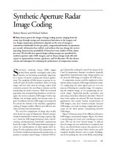
coherency matrix, histograms for each normalized curvelet subbands are cascaded to form a feature vector per pixel. The results show that the proposed HoC feature extraction method gives the best classification accuracies for most of the test setups but when the number of training samples are heavily reduced, SRAD results overtake by means of classification accuracy. In this work using all of the elements of coherency matrix, curvelet subband GD parameters are cascaded to form a feature vector to be used in clustering. Curvelet family for a continuous domain is composed of directional wedge filter results of concentric scales together with a low pass component in the frequency domain. Frequency domain continuous curvelet transform tiling is given with Figure 1a. Continuous curvelet transform Uj,ℓ (r,θ) at scale 2−j (for j ≤ j0) and rotation θℓ in the frequency domain for signals of R2 is defined with ω frequency domain Cartesian variables, r, θ frequency domain polar variables, W radial windowing function and periodic with 2π radians V angular windowing function as in Equation (9). The ranges for the variables can be given as: r ≥ 0, θ ∈ [0, 2π), j ∈ N0, ℓ ∈ N0, θℓ = 2πℓ 2−⌊j/2⌋. j parameter is an element of positive natural numbers and defines a 2−𝑗 scaling for the windowing function, Uj,ℓ term is given to address one of several frequency domain windows at scale 2−j and orientation θℓ. −3𝑗 4 𝑊

𝑈𝑗 ,ℓ 𝑟, θ = 2

2−𝑗 𝑟 𝑉

2⌊𝑗

2⌋

θ − θℓ 2𝜋

(9)

The scale where j ≤ j0 is given as the coarse curvelet represents the low pass component. Coarse curvelet can be given with W0 windowing function in Equation (10). 𝑈𝑗 0 𝛚 = 2−𝑗 0 𝑊0 2−𝑗 0 𝛚

(10)

Figure 1. (a) Continuous curvelet transform frequency domain tiling; (b) Discrete curvelet transform frequency domain tiling.

(a)

(b)

Curvelet transform spatially is given with the Fourier pair of F{φ(x)}=U(ω). φ is obtained as a Gauss filtered oscillating function. All together parabolic scaled (unequal stretching at different axis) with Dj, rotated with Rθℓ and translated with k = (k1, k2) ∈ R2 versions of φ give the spatial curvelet family. The spatial curvelet family can be given in Equation (11).

Remote Sens. 2014, 6

5502

φ𝑗 ,ℓ,𝒌 𝒙 = 𝐷𝑗 φ 𝐷𝑗 𝑅𝜃 ℓ 𝒙 − 𝒌

, 𝑅𝜃 ℓ =

cos θℓ − sin θℓ

𝑗 sin θℓ , 𝐷𝑗 = 2 cos θℓ 0

0 2𝑗 2

(11)

Spatial counterpart of the coarse curvelet can be given in Equation (12). φ𝑗 0 ,𝒌 𝒙 = φ𝑗 0 𝒙 − 2−𝑗 0 𝒌

(12)

Given the spatial curvelet family, curvelet transform coefficients 𝑐 of a continuous signal f is obtained as the inner product of the function and the curvelets as in Equation (13), where φ denotes complex conjugate. 𝑐 𝑗, ℓ, 𝒌 = ⌌𝑓, 𝜑𝑗 ,ℓ,𝒌 ⌍ =

ℝ2

𝑓 𝒙 𝜑𝑗 ,ℓ,𝒌 𝒙 𝑑𝒙

(13)

Taking together into account any two origin reflection curvelets (Uj,ℓ(r,θ) + Uj,ℓ(r,θ + π)) results in real valued curvelet transform coefficients. Discrete curvelet family in the frequency domain is defined as shear filters at concentric square windows as given in Figure 1b. The discrete curvelet transform coefficients cD of a discrete signal f [t1, t2] of size n × n based on spatial discrete curvelet family φD can be given as an inner product in Equation (14). 𝑐 𝐷 𝑗, ℓ, 𝒌 =

𝑓 𝑡1 , 𝑡2 φ𝐷𝑗 ,ℓ,𝒌 𝑡1 , 𝑡2

(14)

0≤𝑡 1 ,𝑡 2 ≤𝑛

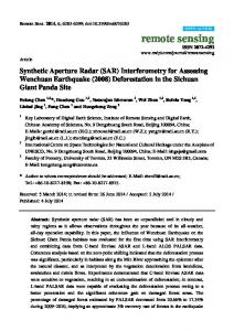
Curvelet transform family spatially is illustrated in Figure 2 with different orientations and scales together with the coarse curvelet presented in the frequency domain and spatially. Figure 2. (a) Discrete curvelet transform coefficients spatially left to right orientations of 3π 4 , π 2 , π 4 , 0, top to bottom scales 4, 3, 2; (b) Discrete coarse curvelet coefficients in the frequency domain; (c) Discrete coarse curvelet coefficients spatially.

(a)

Remote Sens. 2014, 6

5503 Figure 2. Cont.

(b)

(c)

Curvelet-based subband GD parameter estimation feature extraction for SAR image is carried out first with taking the curvelet transform of a window around the pixel of interest. Based on the number of orientations and scales used for curvelet transform, the number of curvelet subbands varies. Feature extraction for a pixel and its neighbors can then be carried out as calculating the mean and standard variation values for each subband and cascading them. Supposing S number of subbands and six elements of the coherency matrix, the number of features for each pixel can be given as 2 × S × 6. Curvelet-based feature extraction is important as it emphasizes spatial locality and can extract agricultural field furrow-like features naturally. 3. Dataset Description and Clustering Methods This section is divided into two subsections mainly focusing on the dataset description and clustering methods used, respectively. 3.1. Dataset Description Test materials for this work are from widely used Flevoland data acquired by AirSAR platform. Flevoland is mostly regained from sea and is located in the middle of the Netherlands as given in Figure 3. Air SAR data of Flevoland is in the form of multispectral (P, L and C bands) full polarimetric (V[ertical]V, VH[orizantal], HV, VV polarizations) modes. The nominal spatial resolution is given between 5 and 10 m. The C band full polarimetric data is used for clustering of crop lands in this work. The region of interest (ROI) area, that is 320 × 200 pixels in size, is given in Figure 3c with false coloring. Ground truth label map of the ROI region is given in Figure 4. Flevoland data is provided in T3 format, which is the average coherency matrix of reduced Pauli decomposition vector for each pixel over number of looks 𝐿. The Pauli decomposition vector k and the definition of coherency matrix Ω can be given in Equations (15) and (16), respectively, based on polarimetric backscattering amplitudes ( 𝑆𝑕𝑕 : horizontally polarized transmitter and horizontally polarized receiver, 𝑆𝑕𝑣 : horizontally polarized transmitter and vertically polarized receiver, 𝑆𝑣𝑕 : vertically polarized transmitter and horizontally polarized receiver, 𝑆𝑣𝑣 : vertically polarized transmitter and vertically polarized receiver). The elements of reduced Pauli decomposition vector

Remote Sens. 2014, 6

5504

correspond to odd bounce scattering, even bounce scattering and volume scattering components, which can be utilized to understand the underlying physical properties of the landcover. 1 𝑆𝑕𝑕 + 𝑆𝑣𝑣 𝑆𝑕𝑕 − 𝑆𝑣𝑣 ∈ ℂ3×1 𝒌= 2 𝑆 +𝑆 𝑕𝑣 𝑣𝑕

(15)

Figure 3. (a) Location of Flevoland test site; (b) False coloring of Flevoland data; (c) False coloring of Flevoland ROI data.

52º19'32"N 52º18'30"N 5º0'0"E

6º0'0"E

52º17'28"N

53º30'0"N 52º30'0"N 52º0'0"N 51º30'0"N

50 km 4º0'0"E

52º20'33"N

45º0'0"N

53º0'0"N

55º0'0"N

1 km

N

52º21'35"N

35º0'0"N

52º22'237"N

N

7º0'0"E

500 km 10º0'0"W

0º0'0"

10º0'0"E

20º0'0"E

(a)

(b)

(c)

Remote Sens. 2014, 6

5505

Figure 4. (a) Flevoland ROI labels; (b) Flevoland ROI class information. Label 0 1 2 3 4 5 6 7 8 9

Class No Labels Bare Soil Grass Sugar Beet Rapeseed Winter Wheat 1 Winter Wheat 2 Lucerne Potatoes Stem Beans

Total # of samples (a)

# of Samples 592 5117 3216 690 1173 4140 1549 5986 442 22,905

(b)

Coherency matrix is formed as the average of Pauli decomposition vector multiplied by its Hermitian (conjugate transpose) over number of looks. The coherency matrix contains second order moments of the scattering process and can be used to describe the correlation properties of natural scatterers [9]. 1 𝛀= 𝐿

𝐿

𝒌ℓ 𝒌ℓ 𝐻

(16)

ℓ=1

Coherency matrix (3 × 3 matrix) is obtained as a Hermitian matrix, which means conjugate transpose of the matrix is equal to itself. For that reason, commercially, SAR data is provided as real diagonal values of the coherency matrix together with real and imaginary parts of the strictly upper triangular matrix. 3.2. Clustering Methods 3.2.1. K-Means Clustering K-means algorithm is defined for clustering 𝑛 distinct samples into total of 𝑐 clusters (𝐺𝑖 , 𝑖 = 1, … , 𝑐). The algorithm minimizes the cost function 𝐽 with respect to optimum 𝑐 cluster centers based on total distance of samples to the cluster centers 𝑐𝑖 that they belong to, given in Equation (17). In Equation (17), 𝑐𝑖 corresponds to the center of mass for clusters and 𝑑 𝑥𝑘 − 𝑐𝑖 to distance between 𝑖’th center and associated 𝑘’th sample. 𝑐

𝐽=

𝑑 𝑥𝑘 − 𝑐𝑖 𝑖=1 𝑘,𝑥 𝑘 ∈𝐺𝑖

(17)

Remote Sens. 2014, 6

5506

K-means associates each sample with one cluster. This can be expressed in Equation (18) with c × n-sized binary membership matrix U, in which each row sums up to 1. Each element 𝑢𝑖𝑗 of the matrix 𝑈 is 1 if the 𝑗’th sample belongs to cluster i and 0 if not. 𝑢𝑖𝑗 = 1, 𝑓𝑜𝑟𝑒𝑎𝑐𝑕 𝑘 ≠ 𝑖 𝑖𝑓 𝑥𝑗 − 𝑐𝑖 0, 𝑒𝑙𝑠𝑒

2

≤ 𝑥𝑗 − 𝑐𝑘

2

(18)

Centers of the clusters are calculated in Equation (19) as the average of the samples of each cluster. Here 𝐺𝑖 shows the number of samples in cluster 𝐺𝑖 . 1 𝐺𝑖

𝑐𝑖 =

𝑥𝑘 𝑘,𝑥 𝑘 ∈𝐺𝑖

(19)

K-means algorithm can be given iteratively as Algorithm 1 [15]. K-means does not guarantee an optimum result as it is heavily dependent on initial cluster centers. Algorithm 1: K-means IN 𝑐, 𝑥𝑗 =1…𝑛 𝑐𝑖 ← randomly selected number of 𝑐 samples from 𝑥𝑗 repeat 𝑢𝑖𝑗 ← calculate membership for each sample 𝑥𝑗 with Equation (18) 𝑐𝑖 ← calculate new cluster centers for each cluster with Equation (19) until 𝐽𝑐𝑢𝑟𝑟𝑒𝑛𝑡 − 𝐽𝑝𝑟𝑒𝑣𝑖𝑜𝑢𝑠 < 𝑡𝑕𝑟𝑒𝑠𝑕𝑜𝑙𝑑 OUT 𝑐𝑖=1…𝑐 3.2.2. Fuzzy C-Means (FCM) Clustering Fuzzy C-means, which utilizes fuzzy valued memberships for clusters, is different from k-means as k-means has strict binary membership values. In FCM, each sample is assigned a membership value for each cluster that sums up to 1 over all clusters per sample. This membership can take values between 0 and 1. Cost function 𝐽 for FCM is given in Equation (20). Here 𝑢𝑖𝑗 defines the fuzzy membership value of sample 𝑗 to cluster 𝑖, whereas 𝑑𝑖𝑗 is the distance from cluster center 𝑐𝑖 to sample 𝑥𝑗 and 𝑚 ∈ 1, ∞ is the fuzzification coefficient. 𝑐

𝑛

𝑢𝑖𝑗 𝑚 𝑑𝑖𝑗 2

𝐽=

(20)

𝑖=1 𝑗 =1

Each cluster center 𝑐𝑖 can be given based on fuzzy membership values 𝑢𝑖𝑗 in Equation (21). 𝑐𝑖 =

𝑛 𝑚 𝑗 =1 𝑢𝑖𝑗 𝑥𝑗 𝑛 𝑚 𝑗 =1 𝑢𝑖𝑗

(21)

Fuzzy membership values 𝑢𝑖𝑗 for each sample can be calculated based on cluster centers 𝑐𝑖 , as in Equation (22). 1

𝑢𝑖𝑗 = 𝑐 𝑘=1

𝑑𝑖𝑗 𝑑𝑘𝑗

2 𝑚 −1

(22)

Remote Sens. 2014, 6

5507

FCM algorithm can be given iteratively as Algorithm 2 [15]. FCM does not guarantee optimum cluster centers as it is heavily dependent on initial fuzzy membership values. Algorithm 2: FCM IN 𝑐, 𝑥𝑗 =1…𝑛 , 𝑚 𝑢𝑖𝑗 ← randomly initialize fuzzy membership values repeat 𝑐𝑖 ← calculate new cluster centers for each cluster with Equation (21) 𝑢𝑖𝑗 ← calculate fuzzy membership foreach sample 𝑥𝑗 with Equation (22) until 𝐽𝑐𝑢𝑟𝑟𝑒𝑛𝑡 − 𝐽𝑝𝑟𝑒𝑣𝑖𝑜𝑢𝑠 < 𝑡𝑕𝑟𝑒𝑠𝑕𝑜𝑙𝑑 OUT 𝑐𝑖=1…𝑐 3.2.3. Spatial Fuzzy C-Means (sFCM) Clustering Spatial fuzzy c-means is defined as diffusion of feature space fuzzy membership values through spatial neighborhood membership values [16]. In each iteration, spatial fuzzy membership values (𝑕𝑖𝑗 ) are calculated based on feature space fuzzy membership values (𝑢𝑖𝑗 ) and those two values are fused together to form the overall fuzzy membership (𝑢𝑖𝑗′ ) of a sample. Spatial fuzzy membership 𝑕𝑖𝑗 of samples for a w × w neighborhood window 𝑁𝐵 can be given in Equation (23) based on feature space fuzzy membership values. 𝑕𝑖𝑗 =

𝑢𝑖𝑘 𝑘∈𝑁𝐵 𝑥 𝑗

(23)

Feature space fuzzy membership values can be fused together with the spatial fuzzy membership values to form fuzzy membership values as in Equation (24) [17]. 𝑢𝑖𝑗′

=

𝑢𝑖𝑗𝑝 𝑕𝑖𝑗𝑞

𝑝 𝑞 𝑐 𝑘=1 𝑢𝑘𝑗 𝑕𝑘𝑗

sFCM algorithm can be given iteratively as Algorithm 3. Algorithm 3: sFCM IN 𝑐, 𝑥𝑗 =1…𝑛 , 𝑚, 𝑁𝐵, 𝑝, 𝑞 𝑢𝑖𝑗 ← randomly initialize fuzzy membership values repeat 𝑐𝑖 ← calculate new cluster centers foreach cluster with Equation (21) 𝑕𝑖𝑗 ← calculate spatial fuzzy membership foreach sample 𝑥𝑗 with Equation (23) 𝑢𝑖𝑗′ ← calculate fuzzy membership foreach sample 𝑥𝑗 with Equation (24) 𝑢𝑖𝑗 ← calculate feature space fuzzy membership foreach sample 𝑥𝑗 with Equation (22) until 𝐽𝑐𝑢𝑟𝑟𝑒𝑛𝑡 − 𝐽𝑝𝑟𝑒𝑣𝑖𝑜𝑢𝑠 < 𝑡𝑕𝑟𝑒𝑠𝑕𝑜𝑙𝑑 OUT 𝑐𝑖=1…𝑐

(24)

Remote Sens. 2014, 6

5508

3.2.4. Two-Dimensional Self-Organizing Maps (2D-SOM) 2D-SOM is a two-dimensional unsupervised clustering algorithm, which can be defined with a four-neighbor rectangular grid or three-neighbor hexagonal grid artificial neural network structure, used to transform the input space into a two-dimensional projection space preserving topology [18]. SOM structure can be given for a total of 𝑀 neurons, 𝑿 ∈ 𝑅 𝑛 𝑛 dimensional input vectors and 𝑤𝑀×𝑛 weights from input layer to neurons. SOM algorithm is an iterative method that updates the most similar neuron to an input and its neighboring neurons’ weights in such a way that resemblance is increased to that input. The most similar neuron at iteration step 𝑡 to an input 𝒙 is called the winning neuron 𝑣 and can be defined with neuron weight 𝒘 as given in Equation (25). Here 𝑆 represents the set of SOM neurons. 𝜈 𝑡 = argmin 𝒙 𝑡 − 𝒘𝑘 𝑡 𝑘∈𝑆

(25)

How much the other neurons (indexed with 𝑘) are to be updated together with the winning neuron (indexed with 𝑣) can be defined with 𝑟𝑖 position vector of i’th neuron, and ς(𝑡) decreasing effective neighbor-distance-function as in Equation (26). 𝜂 𝜈, 𝑘, 𝑡 = 𝑒

−

𝒓𝜈 −𝒓𝑘 2 2ς 2 𝑡

(26)

The weight update can be defined with distance of the input 𝑥 to the winning neuron, neighboring distance of other neurons to the winning neuron and adaptation coefficient 𝑎 as in Equation (27). α can be chosen to be a monotonically decreasing linear, exponential or rational function. ∆𝒘𝑘 𝑡 = 𝛼 𝑡 𝜂 𝜈, 𝑘, 𝑡 [𝒙 𝑡 − 𝒘𝜈 𝑡 ] 𝒘𝑘 𝑡 + 1 = 𝒘𝑘 𝑡 + ∆𝒘𝑘 𝑡

(27)

2D-SOM algorithm can be given iteratively as Algorithm 4 [19]. Algorithm 4: 2D-SOM IN 𝑀, 𝑋, ς, α 𝑤𝑀×𝑛 ← randomly initialize weight values repeat foreach 𝑥𝑖 𝑣𝑖 (𝑡) ← calculate winning neuron with Equation (25) Update winning neuron and its neighboring weights with Equation (27) end for each until ∆𝒘𝑘 𝑡 < 𝑡𝑕𝑟𝑒𝑠𝑕𝑜𝑙𝑑 or (max_number_of_iterations) is reached OUT 𝑤𝑀×𝑛 4. Experimental Results Experiments are conducted for each feature extraction method paired together with the aforementioned clustering methods. For the clustering methods, a number of clusters are chosen to be equal to the number of classes, except for the 2D-SOM, where a higher number of clusters is constructed. In the literature, clustering performance evaluation without ground truth is carried out by

Remote Sens. 2014, 6

5509

cluster validation measures, whereas with ground truth information, accuracy calculation after cluster labeling can be used as a performance measure. In 2D-SOM, each cluster is labeled with the majority of the sample labels, whereas in the rest of the methods labeling is carried out by maximizing the overall accuracy in a one-to-one correspondence manner. Kappa values together with the clustering accuracies according to known labels are given as performance measures. Curvelet subband GD parameter estimation feature extraction is carried out for window size 33 × 33, number of scales 2 and number of orientations 16 (as a result 17 subbands per coherency matrix element). Thus, the number of features per pixel can be given as 204 (17 subbands × 6 elements of coherency matrix × 2 features) for curvelet subband GD parameter estimation. This method is denoted in the tables as μ, ς. It should also be noted that curvelet subband features are normalized feature-wise prior to being fed to clustering methods. Experimental results are presented in two forms based on clustering accuracies and clustering maps. Clustering accuracies are given according to overall accuracies and Kappa values are able to assess the performance of the proposed feature extraction method compared with standard benchmark features. Clustering accuracies are also further analyzed for higher number of clusters for clustering methods (k-means, FCM, sFCM) that practically use the same number of clusters as class labels. Clustering maps are given in order to be able to provide visual comparison between feature extraction methods on each clustering method. 4.1. Accuracies and Errors K-means clustering accuracies are given in Table 1 for the average of 20 runs for each feature extraction method. The best clustering accuracy is achieved for SRAD features with k-means algorithm up to 65.41% with the experiments. Table 1. K-means overall clustering accuracies. Feature Extraction ORG SRAD H/A/𝛂 𝛍, 𝛔

Clustering Accuracy (%) 38.06 65.41 44.68 44.50

FCM clustering overall accuracies are given in Table 2 for the average of 20 runs. It can be seen from Table 2 that clustering overall accuracies can be increased compared to hard membership k-means, with the introduction of fuzzy cluster memberships. It should also be noted that as the 𝑚 value increases, the threshold constraint is met at a small number of iterations. Feature extraction methods can be ordered with respect to clustering accuracies as SRAD, μ, ς features, original data and H/A/α for FCM method. sFCM clustering method results are calculated for a fixed fuzzy membership value (m = 2), various feature-space and spatial fuzzy membership values (𝑝, 𝑞 ∈ 0,1,2,4,8 ) and different window sizes (𝑤 ∈ 5,11,21 ). sFCM results of the 20-run averages for best clustering accuracy yielding parameters are given in Table 3. Compared to k-means and FCM, it can be said that the introduction of spatial information through clustering iterations with sFCM, enhanced clustering accuracy for H/A/α more

Remote Sens. 2014, 6

5510

than the curvelet subband µ, σ features. The best clustering accuracy for sFCM is achieved by SRAD features up to 85.11%.

Overall accuracies for different 𝒎 values (%)

Table 2. FCM overall clustering accuracies. 𝒎 Values 1.1 1.2 1.4 2 3 4 8 16 32 64

ORG 37.86 38.02 38.15 38.68 40.00 39.99 42.57 47.58 43.99 40.85

Feature Extraction SRAD H/A/𝛂 66.42 44.58 66.64 44.52 63.05 44.40 59.17 43.23 51.92 39.63 50.11 41.04 52.14 43.65 65.64 46.16 65.17 42.06 62.52 41.53

𝛍, 𝛔 48.66 48.72 49.33 48.42 43.25 40.72 38.53 47.95 47.49 48.63

Table 3. The best sFCM overall clustering accuracies for fixed 𝑚 = 2 and corresponding parameter values. Feature Extraction

Clustering Accuracy (%)

ORG SRAD H/A/𝛂 𝛍, 𝛔

47.49 85.11 67.29 61.98

𝒑 𝒒

𝒘

0 4 0 0

11 21 21 21

1 2 2 8

2D-SOM clustering results are calculated for 7 × 7, 9 × 9, 11 × 11 and 13 × 13-sized hexagonal grid networks and 3, 4, 5 and 6 initial neighborings respectively. 2D-SOMs run for 1000 iterations and resulting clusters are labeled as the majority label they contain. In Table 4, overall clustering accuracies are given together with the number of unique labels assigned in parenthesis. SRAD features with 7 × 7 and 9 × 9 SOM networks have better clustering accuracies compared to µ, σ features, whereas as the network grows µ, σ features presents better accuracies. It can be inferred from the results in Table 4 that SRAD extracts similar features and curvelet subband GD parameter estimation extracts discriminating features. Thus with SRAD as the network grows, 2D-SOM cannot set previously clustered together samples apart clearly. On the other hand, with µ, σ features, as the network grows and the number of clusters increases, the use of discriminating features results in labeled samples falling into similar clusters. The confusion matrices results from 2D-SOM with 13 × 13 topology for SRAD and curvelet subband µ, ς features are given in Tables 5 and 6, respectively.

Remote Sens. 2014, 6

5511 Table 4. 2D-SOM overall clustering accuracies.

Feature Extraction ORG SRAD H/A/𝛂 𝛍, 𝛔

7 × 7 SOM 61.36 (4) 89.29 (9) 60.90 (8) 86.24 (9)

Accuracies (%) for SOM Size 9 × 9 SOM 11 × 11 SOM 13 × 13 SOM 62.13 (6) 63.15 (6) 64.28 (7) 90.09 (9) 91.59 (9) 91.90 (9) 61.89 (8) 62.82 (9) 63.39 (9) 89.68 (9) 93.00 (9) 94.94 (9)

Table 5. Cluster confusion matrix for SRAD features. Actual Labels 1 2 3 4 5 6 7 8 9

1 567 21 1 1 2 5 0 0 0

2 19 4773 16 3 10 105 670 4 12

3 0 24 3107 13 18 15 35 151 2

SRAD Cluster Labels 4 5 6 0 0 6 2 3 100 3 5 13 653 7 13 9 1010 114 28 63 3902 0 0 19 1 0 6 0 0 0

7 0 194 25 0 6 17 825 0 0

8 0 0 41 0 3 2 0 5786 2

9 0 0 5 0 1 3 0 38 426

Total Samples 592 5117 3216 690 1173 4140 1549 5986 442

Table 6. Cluster confusion matrix for curvelet subband μ, ς features. Actual Labels 1 2 3 4 5 6 7 8 9

1 506 31 0 0 0 0 0 0 0

2 65 4850 54 0 0 16 284 16 2

3 0 41 3098 0 22 16 128 20 0

𝛍, 𝛔 Cluster Labels 4 5 6 0 0 12 0 0 1 6 0 1 690 0 0 1 1091 33 30 0 4078 0 0 64 0 3 0 0 0 0

7 9 109 54 0 0 0 1059 13 0

8 0 51 3 0 26 0 14 5934 0

9 0 34 0 0 0 0 0 0 440

Total Samples 592 5117 3216 690 1173 4140 1549 5986 442

The most confused labels and the number of confusions for SRAD with 13 × 13 2D-SOM can be listed as (label1–label2: sum of # of mislabeled samples): 2–7:864 (670 + 194), 2–6:205, 3–8:192, 5–6:177. The most confused labels and the number of confusions for curvelet subband µ, σ features with 13 × 13 2D-SOM can be listed as (label1–label2: sum of # of mislabeled samples): 2–7:393, 3–7:182, 1–2:96. The most mislabeling occurs with labels 2 (grass) and 7 (lucerne), which can be considered alike by means of vegetation structure and therefore by SAR backscattering mechanism. This result can also be seen in 2D-SOM spatial node labels, where almost the only neighbors for Lucerne-labeled clusters are grass-labeled clusters. Kappa values for the best clustering accuracies are given in Table 7. Kappa value can be considered as differentiation from the expected value of random labeling accuracies and is given as Equation (28),

Remote Sens. 2014, 6

5512

where 𝑃(𝑎) is the confusion matrix accuracy probability and 𝑃(𝑒) is the probability of random labeling. Overall the best Kappa value as 0.9382 is reached with the use of µ, σ features in 13 × 13 topology 2D-SOM. SRAD features again with 13 × 13 topology-SOM are placed second with Kappa value 0.9009. 𝜅=

𝑃 𝑎 −𝑃 𝑒 1−𝑃 𝑒

(28)

Table 7. Kappa values. ORG

SRAD

H/A/𝛂

𝛍, 𝛔

K-Means

0.2521

0.5329

0.3686

0.3614

FCM

0.3237

0.6106

0.3135

0.4111

sFCM

0.3491

0.8350

0.6223

0.5492

Clustering Methods

Features

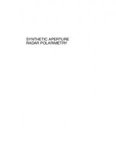
Overall evaluation of feature extraction methods on k-means, FCM and sFCM together with 2D-SOM is also carried out with higher number of clusters for 20 runs. That is k-means, FCM, sFCM are evaluated with 50, 100 and 150 clusters and labels are given the same way as in 2D-SOM. FCM is run for 𝑚 = 2, sFCM is run for 𝑚 = 2, 𝑝 = 1, 𝑞 = 1 and 𝑤 = 21. The results are given in graphical form with x-axis showing number of clusters and y-axis showing accuracies as in Figure 5. Figure 5. Comparison of accuracies of feature extraction methods on (a) k-means; (b) FCM; (c) SRAD and (d) 2D-SOM, with different number of clusters.

(a)

(b)

(c)

(d)

Remote Sens. 2014, 6

5513

It can be seen from the graphs in Figure 5 that curvelet subband µ, σ features starts with slightly lower accuracy compared to SRAD in all clustering methods; however, with the increasing number of clusters curvelet subband µ, σ features reach up to the SRAD accuracies. In 2D-SOM clustering curvelet subband µ, σ features gives even better accuracies compared to SRAD. The sFCM method is also run with 169 clusters for SRAD and curvelet subband µ, σ features, and accuracies of 94.82% and 94.67% are obtained respectively. The best accuracy overall is obtained by 13 ×13 2D-SOM with curvelet subband µ, σ features with 94.94%. These results are also consistent with nine cluster results of k-means, FCM and sFCM. Practically, feature extraction in SAR images is conducted following a speckle noise reduction step. However, the proposed feature extraction method can be carried out without speckle reduction, as it utilizes spatial features naturally by curvelet transform. Moreover as the curvelet subband features are extracted on averages and standard deviations the disturbing effect of speckle noise can be eliminated to some extent. Results from Table 1 to Table 4 and graphs from Figure 5 suggest that the proposed method is as accurate as SRAD features or even better at some experimental setups thereby demonstrating that the proposed method is robust against speckle noise. 4.2. Clustering Maps K-means clustering maps are given in Figure 6 together with labels and the label map. Using only feature space hard memberships and similarity measures to cluster centers, k-means clustering mappings result in cluttered small regions for original data and H/A/α, whereas bigger homogeneous regions can be seen for SRAD and µ, σ features where spatial information is diffused through feature extraction. Figure 6. K-means clustering maps for (a) original data; (b) SRAD; (c) H/A/α; (d) curvelet subband µ, σ features; (e) Label map and (f) class labels.

(a)

(b)

(c)

Remote Sens. 2014, 6

5514 Figure 6. Cont.

Label Class 1 Bare Soil 2 Grass 3 Sugar Beet 4 Rapeseed 5 Winter Wheat 1 6 Winter Wheat 2 7 Lucerne 8 Potatoes 9 Stem Beans

(d)

(e)

(f)

FCM clustering maps for the best clustering accuracy yielding 𝑚 values are given in Figure 7 together with labels and the label map. In Figure 7, clustering maps are given for original data with 𝑚 = 16, SRAD with 𝑚 = 1.2, H/A/α features with 𝑚 = 16 and curvelet subband GD µ, σ parameter estimation features with 𝑚 = 1.4. Figure 7. The best overall accuracy yielding FCM clustering maps for (a) original data; (b) SRAD; (c) H/A/α; (d) curvelet subband μ, σ features; (e) Label map and (f) class labels.

(a)

(b)

(c)

Remote Sens. 2014, 6

5515 Figure 7. Cont.

Label 1 2 3 4 5 6 7 8 9

(d)

(e)

Class Bare Soil Grass Sugar Beet Rapeseed Winter Wheat 1 Winter Wheat 2 Lucerne Potatoes Stem Beans

(f)

sFCM clustering maps for the best clustering accuracy yielding parameters are given in Figure 8 together with labels and the label map. Apart from spatial information being diffused by feature extraction in SRAD and curvelet µ, σ features, the introduction of spatial information through sFCM clustering steps also enables bigger homogeneous-labeled regions for all feature extraction methods. Figure 8. The best overall accuracy yielding sFCM clustering maps for (a) original data; (b) SRAD; (c) H/A/α; (d) curvelet subband μ, σ features; (e) Label map and (f) class labels.

(a)

(b)

(c)

Remote Sens. 2014, 6

5516 Figure 8. Cont.

Label 1 2 3 4 5 6 7 8 9

(d)

(e)

Class Bare Soil Grass Sugar Beet Rapeseed Winter Wheat 1 Winter Wheat 2 Lucerne Potatoes Stem Beans

(f)

2D-SOM classification maps for 13 × 13 topologies are given in Figure 9. In analyzing 2D-SOM cluster mapping for SRAD, it can be seen that confusions in the labeling mostly occur at edges of the regions. This situation can be explained with SRAD preserving edges by definition. Cluster confusion can also be seen due to feature diffusion in neighboring regions both in SRAD and µ, σ features. Figure 9. The 13 × 13 topology 2D-SOM clustering maps for (a) original data; (b) SRAD; (c) H/A/α; (d) curvelet subband μ, σ features; (e) Label map and (f) class labels.

(a)

(b)

(c)

Remote Sens. 2014, 6

5517 Figure 9. Cont.

Label 1 2 3 4 5 6 7 8 9

(d)

(e)

Class Bare Soil Grass Sugar Beet Rapeseed Winter Wheat 1 Winter Wheat 2 Lucerne Potatoes Stem Beans

(f)

2D-SOM nodes labeled as their majority labels are given in Figure 10 for 13 × 13 topology with consistent coloring from cluster mappings. This figure illustrates 2D-SOM node label neighborhood and gives insight for cluster label confusion. Figure 10. The 13 × 13 topology 2D-SOM node labels (a) original data; (b) SRAD; (c) H/A/α; (d) curvelet subband μ, σ features and (e) SOM node label legend.

(a)

(b)

(c)

(d)

Bare Soil Grass Sugar Beet Rapeseed Winter Wheat 1 Winter Wheat 2 Lucerne Potatoes Stem Beans

(e)

5. Conclusions Unsupervised clustering is an important field of study in synthetic aperture radar (SAR) remote sensing. This study mainly focuses on curvelet-based feature extraction for clustering SAR images. The proposed method is based on defined multidirectional and multiscale curvelet transform that enables sparse representations for signals. The implementation originates from the method proposed in content-based image retrieval (CBIR) classification field and is based on curvelet subband Gauss

Remote Sens. 2014, 6

5518

distribution (GD) µ, σ parameter estimation feature extraction. Therefore, the uniqueness of the study can be stated as the use of curvelet subband Gauss distribution µ, σ parameter estimation for feature extraction in clustering. Curvelet subband GD parameter estimation features are compared against original data, H/A/α polarimetric decomposition and speckle reduced data features with k-means, fuzzy c-means (FCM), spatial fuzzy c-means (sFCM) and two-dimensional self-organizing maps (2D-SOM) clustering methods by means of effect on clustering accuracy on a test site with ground truth information. The speckle reducing anisotropic diffusion (SRAD) method reveals the best clustering accuracies for k-means, FCM, sFCM and small-sized 2D-SOMs. Curvelet subband µ, σ features give the best clustering accuracies for bigger 2D-SOMs, which are also the best clustering accuracy overall as 94.94%. The results suggest that SRAD-based features can be considered as extracting similar features among samples, whereas curvelet-based features can be considered as extracting discriminating features. These results mainly rely on the test site restrictions which can be listed as: having low relief angle, and the land being suitable for land use classification. Apart from the discussed clustering methods, hierarchical clustering methods are also expected to perform well with discriminating features from curvelet subband GD parameter estimation. Also, as future work, feature selection and feature reduction can be implemented to the extracted curvelet subband features to increase accuracy. Author Contributions Both authors contributed extensively to the work presented in this paper. Conflicts of Interest The authors declare no conflict of interest. References 1.

2. 3. 4.

5.

Yu, P.; Qin, A.K.; Clausi, D.A. Unsupervised polarimetric SAR image segmentation and classification using region growing with edge penalty. IEEE Trans. Geosci. Remote Sens. 2012, 50, 1302–1317. Gan, L.; Wu, Y.; Wang, F.; Zhang, P.; Zhang, Q. Unsupervised SAR image segmentation based on Triplet Markov fields with graph cuts. IEEE Geosci. Remote Sens. Lett. 2013, 11, 853–857. Zhang, X.; Jiao, L.; Liu, F.; Bo, L.; Gong, M. Spectral clustering ensemble applied to SAR image segmentation. IEEE Trans. Geosci. Remote Sens. 2008, 46, 2126–2136. Li, Y.; Li, J.; Chapman, M.A. Segmentation of SAR intensity imagery with a Voronoi tessellation, Bayesian inference, and reversible jump MCMC algorithm. IEEE Trans. Geosci. Remote Sens. 2010, 48, 1872–1881. Peng, R.; Wang, X.; Lü, Y.; Wang, S. SAR Imagery Segmentation Based on Integrated Active Contour. In Proceedings of the 2nd International Conference on Advanced Computer Control (ICACC), Shenyang, China, 27–29 March 2010; pp. 43–47.

Remote Sens. 2014, 6 6.

7.

8.

9. 10. 11. 12. 13. 14. 15.

16. 17. 18. 19.

5519

Dabboor, M.; Collins, M.J.; Karathanassi, V.; Braun, A. An unsupervised classification approach for polarimetric SAR data based on the Chernoff distance for complex Wishart distribution. IEEE Trans. Geosci. Remote Sens. 2013, 51, 4200–4213. Yin, J.; Yang, J. Wishart Distribution Based Level Set Method for Polarimetric SAR Image Segmentation. In Proceedings of the International Conference on Electronics, Communications and Control (ICECC), Ningbo, China, 9–11 September 2011; pp. 2999–3002. Yan, X.; Jiao, L.; Xu, S. SAR Image Segmentation Based on Gabor Filters of Adaptive Window in Overcomplete Brushlet Domain. In Proceedings of the 2nd Asian-Pacific Conference on Synthetic Aperture Radar (APSAR 2009), Xi’an, China, 26–30 October 2009; pp. 660–663. Ouchi, K. Recent trend and advance of synthetic aperture radar with selected topics. Remote Sens. 2013, 5, 716–807. Yu, Y.; Acton, S.T. Speckle reducing anisotropic diffusion. IEEE Trans. Image Process. 2002, 11, 1260–1270. Ma, J.; Plonka, G. The curvelet transform. IEEE Signal Process. Mag. 2010, 27, 118–133. Candès, E.; Demanet, L.; Donoho, D.; Ying, L. Fast discrete curvelet transforms. Multiscale Model. Simul. 2005, 5, 861–899. Gomez, F.; Romero, E. Rotation invariant texture characterization using a curvelet based descriptor. Pattern Recognit. Lett. 2011, 32, 2178–2186. Uslu, E.; Albayrak, S. Curvelet-based synthetic aperture radar image classification. IEEE Geosci. Remote Sens. Lett. 2014, 11, 1071–1075. Amasyal, M.F.; Albayrak, S. Fuzzy C-Means Clustering on Medical Diagnostic Systems. In Proceedings of the 12th International Turkish Symposium on Artificial Intelligence and Neural Networks (TAINN 2003), Canakkale, Turkey, 2–4 July 2003. Chuang, K.-S.; Tzeng, H.-L.; Chen, S.; Wu, J.; Chen, T.-J. Fuzzy c-means clustering with spatial information for image segmentation. Comput. Med. Imaging Graph. 2006, 30, 9–15. Li, B.N.; Chui, C.K.; Chang, S.; Ong, S.H. Integrating spatial fuzzy clustering with level set methods for automated medical image segmentation. Comput. Biol. Med. 2011, 41, 1–10. Yin, H. The Self-Organizing Maps: Background, Theories, Extensions and Applications. In Computational Intelligence: A Compendium; Springer: Berlin, Germany, 2008; pp. 715–762. Kohonen, T. Self-Organizing Maps, 3rd ed.; Springer: Berlin, Germany, 2001; Volume 30.

© 2014 by the authors; licensee MDPI, Basel, Switzerland. This article is an open access article distributed under the terms and conditions of the Creative Commons Attribution license (http://creativecommons.org/licenses/by/3.0/).