Design,â AMTA Symposium 2004. [2] Charvat, G.L., âA Unique Approach to Frequency-. Modulated Continuous-Wave Radar Design.â East. Lansing MI: A thesis, ...
SYNTHETIC APERTURE RADAR IMAGING USING A UNIQUE APPROACH TO FREQUENCY-MODULATED CONTINUOUS-WAVE RADAR DESIGN Gregory L. Charvat, MSEE, Leo C. Kempel, Ph.D. Department of Electrical and Computer Engineering Michigan State University 2120 Engineering Building East Lansing, MI 48825 2. The Unique Approach to FMCW Radar ABSTRACT A uniquely inexpensive solution to Frequency-Modulated Continuous-Wave (FMCW) radar was developed, using low cost Gunn oscillator based microwave transceiver modules. However these transceiver modules have stability problems causing them to be unsuitable for use in precise FMCW radar applications, when just one module is used. In order to overcome this problem, a unique radar solution was developed which uses a combination of 2 transceiver modules to create a precise FMCW radar system. This FMCW radar system was then used in a small Synthetic Aperture Radar (SAR) imaging system. The SAR imaging system was composed of a 12 foot long linear track to which the FMCW radar system was mounted. The FMCW radar system would traverse the linear track, acquiring data to be used for producing SAR imagery. The combination of the small aperture length, narrow bandwidth transmit chirp, and overall frequency instability of the FMCW radar system created a number of SAR imaging problems which were unique in this application. However, it was found that when these issues were properly addressed it was possible to create SAR imagery on a low budget.
The unique approach to FMCW radar design is based entirely around the use of two inexpensive microwave transceiver modules. These modules are Gunn diode based, and are more commonly known as ‘Gunnplexers.’ The microwave transceiver module in use for this system is the M/A-Com model MA87127-1 X-band microwave transceiver module. The MA87127-1 is composed of three major components, a voltage controlled oscillator (VCO), mixer, and circulator as shown in figure 3. The VCO is fed into port 1 of the circulator. Port 2 of the circulator is connected to the WR-90 waveguide flange input/output port of the transceiver. Port 3 of the circulator is connected to the RF input of the mixer. Some power is coupled off the VCO and fed into the Local Oscillator (LO) port of the mixer. The IF output of the mixer is connected to a small solder terminal on the outer case of the transceiver.
Keywords: FMCW, Gunn Oscillator, SAR, Linear SAR, Radar Imaging, Small Aperture SAR 1. Introduction A unique approach to FMCW radar was previously introduced in [1] and [2]. Using this radar system, the implementation of two SAR imaging algorithms was studied. These include a range stacking algorithm, and Polar Format Processing based methods. Section 2 explains the theory and operation of the unique approach to FMCW radar. Section 3 describes the SAR system used to acquire range profile data used in testing the algorithms. Section 4 is a discussion of the range stacking algorithm, its implementation, and resulting imagery. Section 5 is a discussion on using a Polar Format Processing based imaging method and its implementation. Conclusions and potential future work are discussed in section 6.
Figure 3: MA87127-1 block diagram. VCO1 is a varactor controlled Gunn diode oscillator. A varactor diode is placed inside of a cavity Gunn oscillator as shown in figure 4. A bias voltage on the varactor diode between, roughly, 0 and 20 V controls the frequency of the Gunn oscillator. A second bias voltage of approximately 10 V is needed to cause the Gunn diode to oscillate at the frequency of the cavity that it is placed in.
Figure 5: Simplified block diagram of the unique FMCW radar solution. Figure 4: MA87127-1 Physical Layout. CPLR1 is a symbolic representation of the coupling action that occurs between the Gunn oscillator diode and the Schottky mixer diode placed within close proximity (see figure 4). MXR1 is created by the coupled power from the Gunn diode oscillator. This coupled power causes the Schottky mixer diode to switch on and off. This switching action causes the Schottky mixer diode to operate as a single balanced mixer. CIRC1 is a ferrite circulator placed inside of the resonant waveguide cavity that contains VCO1 and MXR1. CIRC1 is basically a large magnet precisely placed inside of the resonant cavity. CIRC1 causes RF power from VCO1 to exit the input/output port, and causes RF power coming into the input/output port to be transferred into MXR1. When looking at figure 3, it appears as though one transceiver module alone can be utilized as an FMCW radar system. However, it was found in lab tests that the pass band of the IF port on MXR1 starts to roll off around 1 MHz, causing little to no response at audio frequency, which is were most beats from a short range FMCW radar system will be located. The transceiver module’s receiver worked most efficiently at IF frequencies above 30 MHz, where the loss due to the mixer was found to be the least. The lack of an acceptable low frequency to near DC response from MXR1 renders one individual transceiver module useless for most short range FMCW radar applications. This problem is common for most microwave transceiver modules of this type. Regardless of its shortcomings, when two MA87127-1 (or similar) transceiver modules are used, the unique FMCW radar design solution can be obtained.
A simplified block diagram of the unique FMCW radar solution is shown in figure 5. XCVR1 is centered at frequency f 1 and FM modulated with a linear chirp, kf d , where
k=
volts . sec ond
The output of XCVR1 is
represented with the equation:
TX 1 (t ) = Ac cos[2!f1t + 2!kf d ]
(1)
The output of XCVR1 is fed into the transmit antenna. The transmitted signal is reflected off of the target. The target is situated at a range R and moving at a velocity v (if it is moving). The range R and velocity v correspond to a time difference and Doppler shift between the original transmit signal and that which was picked up by the receive antenna and fed into XCVR2. This time difference corresponds to a beat frequency difference f b as was proven in section 2. Thus, the reflected signal from the target is represented by the equation:
TX 1b (t ) = Ac cos[2!f1t + 2!kf d + 2!f b t ] (2) XCVR2 is set to a fixed frequency of f 2 . XCVR2 is radiating a fixed frequency carrier at that frequency which can be represented by the equation: TX 2 t = Ac cos 2!f 2 t (3)
()
[
]
As explained earlier, the IF output of each transceiver module is a product of its VCO frequency and any RF power that is coming into the input/output port of the module. Because of this, the IF output of XCVR2 can be calculated:
IF2 (t ) = TX 1b (t )TX 2 (t )
two sinusoidal signals. Therefore the video output of the radar system can be expressed as:
Ac2 cos[2!f1t + 2!kf d t + 2!f b t + 2!f 2 t ]+ 2 A2 + c cos[2!f1t + 2!kf d t + 2!f b t " 2!f 2 t ] 2 =
Video Output (4)
The higher frequency term can be dropped. This is a practical consideration since the IF output port of the transceiver modules is not capable of producing X-band microwave signals. Thus, the IF output of XCVR2 can be simplified as:
A2 IF2 (t ) = c cos[2!f1t + 2!kf d t + 2!f b t " 2!f 2 t ] 2 (5) Simultaneously, some power from XCVR2 is coupled into XCVR1, taking advantage of a coupling problem that would otherwise limit a typical FMCW radar system. Power from XCVR2 is deliberately coupled out using CPLR2 and output through ATT1, CIRC1, and into CPLR1. The coupled power injected into CPLR1 is fed into XCVR1. The resulting frequency response at the IF port of XCVR1 is calculated using the equation:
=
Ac4 cos[2!f b t ] 4
(9)
It is clear from the equation above, that the video output is the beat frequency difference f b due to distance from target R and velocity of target v. Thus, we have an FMCW radar system using two inexpensive microwave transceiver modules. 3. SAR System Implementation The unique solution to FMCW radar device used for this paper is shown in figure 6. This system has the following specifications: Center Frequency = 10.25 GHz Chirp Bandwidth = 70 MHz Transmit Power = 10 dBm Front end Noise Figure = 10 dB
IF1 (t ) = TX 2 (t )TX 1 (t ) 2 c
A cos[2!f 2 t + 2!f1t + 2!kf d t ]+ 2 A2 + c cos[2!f 2 t " 2!f1t " 2!kf d t ] 2 =
(6) Like XCVR2, the higher frequency term can be dropped. Thus, the IF output of XCVR1 can be simplified as:
IF1 (t ) =
Ac2 cos[2!f 2 t " 2!f1t " 2!kf d t ] 2 (7)
()
IF1 t is fed into the input port of a limiting amplifier, LIM1. The output of LIM1 is used as the LO drive of MXR1. IF2 t is fed into the input port of an LNA, which is represented by LNA1. The output of LNA1 is fed into the RF input port of MXR1. IF1 t and IF2 t are multiplied together in MXR1. The IF output of MXR1 is amplified by a video amplifier. The resulting product from MXR1 can be represented by the equation: Video Output = IF1 t IF2 t (8)
()
()
()
() ()
The IF port of MXR1 is not capable of reproducing the high frequency terms resulting from the multiplication of
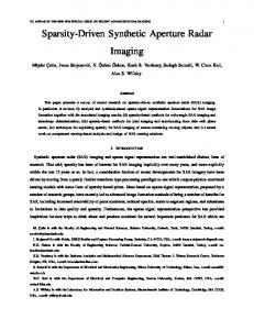
Figure 6: The unique solution to FMCW radar. This radar was mounted on a carrier which traversed a 12 foot long linear SAR track. The transmit and receive antennas were directed perpendicular to the track towards the image scene (see figure 7). A picture of this setup is shown in figure 8.
Figure 7: Experimental setup of linear SAR imaging system.
1 14 27
3500-4000
40
3000-3500
53 66 79
2500-3000 2000-2500 1500-2000 1000-1500
92
500-1000
105
0-500
S105
S79
S92
S53
S66
S27
S40
S1
S14
118
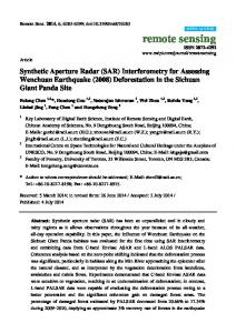
Figure 10: 20 dBsm target located at a distance of 25 ft, and a 30 dBsm target located at 30 ft from the linear SAR track. Figure 8: Picture of SAR experimental setup. This particular experiment was performed indoors. Shown in the foreground is the linear SAR track, and in the background are two standard radar targets. Data acquisition was performed using a National Instruments PCI6014 data acquisition card. A Labview VI was programmed to control data acquisitioning and some pre-processing. Data acquisition was triggered by two inputs. The first input results from the VI prompting the user to move the radar 1 inch down the track. After this is performed, the user hits enter. The VI then waits for an external hardware trigger from a pulse generator. On the rising edge of this trigger, the data acquisition card simultaneously modulates the radar with a linear ramp and digitizes the video output of the radar unit storing the range profile in a 2-D data file. 2000 samples of the video output of the radar unit are digitized at a rate of 200 KSPS. This process is performed every 1 inch until the radar has traversed the entire 12 foot long track.
4. Range Stacking Algorithm A range stacking algorithm was implemented directly from [3]. The system setup and data acquisition procedure described in section 3 was used to acquire data indoors on two standard radar targets. One target was a 30 dBsm trihedral corner reflector located 30 feet from the track. The other target was a 20 dBsm trihedral corner reflector located 25 feet from the track. Resulting SAR imagery is shown in figure 9.
SAR imagery was successfully created using a range stacking algorithm. However, it may be possible to create a more focused image by trying a more advanced technique. 5. Polar Format Processing Polar format processing based algorithms from [4] were studied. Most notably, a narrow beamwidth and narrow bandwidth assumption algorithm was implemented. And more precise algorithms were researched. The video output of the radar system was digitized at 1 inch intervals across the entire 12 foot long linear SAR track. Video data was acquired at 200 KSPS, with a total of 2000 samples for each range profile. Coherent integration was performed 10 times before the radar was moved to the next position. In order to implement this algorithm, complex data (I and Q) had to be extracted from the video output of the radar system. Unfortunately, due to the unusual structure of the LO signal chain in the radar system, using a low cost I and Q demodulator was not an option. Therefore, the video output was over sampled by a factor of 20, allowing a software I and Q demodulation scheme to be implemented. This software I and Q demodulator was done using simple discrete multiplication and filtering techniques [5]. The resulting complex data was then decimated by a factor of 20 in order to ease computation load. A defined scene center at 30’ down range and 6’ cross range was defined, and used to create a matched filter. The data was then multiplied by the matched filter.
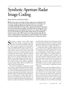
A Fourier transform was taken in the cross range domain. The frequency data was then plotted in the wave number domain to examine the viability to take an evenly spaced 2-D Fourier transform for image formation. The k x and
k y wave number domain plot is shown in figure 11. From [4], the wave number equations were used:
2"f c k x = 2k cos ! n k=
(10)
k y = 2k sin ! n Where:
f = instantaneous transmit frequency of radar unit
For these reasons, it was decided to use the narrow beamwidth and narrow bandwidth approximation to obtain some initial imagery [4]. This assumes that the transmit bandwidth is relatively narrow compared to the center frequency of the radar, which is true for this case. It also assumes that the aperture bandwidth (the k y bandwidth) is also narrow. This is not true, but for this case it was decided to attempt a crude image. The resulting image is shown in figure 12, where a 30 dBsm trihedral corner reflector was placed at 60 ft downrange, and a 20 dBsm trihedral corner reflector was placed at 30 ft down range. Data for this image was acquired outdoors.
c = speed of light
Figure 11:
In order to achieve image formation, a 2-D Fourier transform of this data must be taken. However, the data is not evenly spaced. Therefore interpolation techniques could be used. However, the data shown in figure 11 is not planar, thus not allowing a 2-D Fourier transform to be performed on the entire array of data at one time. Only small chunks of data can accurately be processed.
k x and k y wave number domain plot of acquired data, units in rad/m.
As shown in figure 11, the cross range
k y domain
occupies a wide bandwidth, approximately -80 to 80 rad/m. This fairly wide aperture bandwidth is due to the small aperture size of this radar system, which in this case is only 12 feet long. The downrange k x wave numbers occupy a narrow bandwidth of approximately 11 rad/m but at a very large wave number of approximately 425.5 rad/m. This is due to the narrow 70 MHz transmit bandwidth of the radar system centered at a frequency of 10.25 GHz. Due to the lack of frequency stability of the Gunn diode based microwave devices, the center frequency of 10.25 GHz is only an approximation, and will often drift due to temperature variations and age of the oscillator’s cavity. Consequently, this is always a cause of uncertainty with any SAR image processing using the unique approach to FMCW radar.
Figure 12: Radar imagery created using polar format processing and the narrow bandwidth and narrow beamwidth assumptions. This imaging technique proved to be successful. However, the resulting image in figure 12 suffers from some smearing in the downrange. There is also a potential antenna ringing problem occurring close to the linear SAR track. This is likely due to the front end electronics and parasitic coupling. Further results and attempts to improve the imagery will be presented at the conference. 6. Conclusions and Future Work The unique approach to FMCW radar has been proven successful at creating radar imagery using various
algorithms. Frequency stability, and lack of transmit bandwidth are a continued problem but one that must be dealt with in order to use such a low cost technology. Calibration of this system should be researched. Some potential future work for this project would be to develop commercial applications for this low cost radar imaging system. 7. References [1] Charvat, G.L., Kempel, L. C., “A Unique Approach to Frequency-Modulated Continuous-Wave Radar Design,” AMTA Symposium 2004. [2] Charvat, G.L., “A Unique Approach to FrequencyModulated Continuous-Wave Radar Design.” East Lansing MI: A thesis, submitted to Michigan State University, 2003, in partial fulfillment of the requirements for the degree of Master of Science. [3] Stimson, G.W., “Introduction to Airborne Radar.” El Segundo, California: Hughes Aircraft Company, 1983. [4] Soumekh, M., “Synthetic Aperture Radar Signal Processing With MATLAB Algorithms.” New York: John Wiley & Sons, Inc., 1999. [5] R. E. Ziemer, and W. H. Tranter, “ Principles of Communications, Systems, Modulation, and Noise, 4th Edition.” New York: John Wiley & Sons, Inc., 1995.