f A; B j A = BBT ABBT g is Zariski closed in S n O n; m and consequently of measure zero 11 . Thus, either there exists a matrix pair A; B 2 S n O n; m and ma-.
Journal of Mathematical Systems, Estimation, and Control Vol. 5, No. 2, 1995, pp. 1{32
c 1995 Birkhauser-Boston
System Assignment and Pole Placement for Symmetric Realisations� R.E. Mahony
U. Helmke
y
y
Abstract
In this paper we consider the problem of system assignment for the class of linear output feedback systems having symmetric state space realisations. For such systems the classical pole placement task can be considered as a degenerate case of a more general system assignment problem. It is shown that a symmetric state space realisation can be assigned arbitrary (real) poles via output feedback if and only if there are at least as many system inputs as states. The task of computing feedback gains for system assignment is approached by deriving gradient ows which minimize suitable least squares distance functions on smooth manifolds of output feedback equivalent realisations. These ordinary di�erential equations provide insight into the complex structure of the systems assignment and pole placement problems. Computing the limiting values of the
ows provides a method of determining optimal feedback gains for the system assignment (pole placement) problem even when exact solutions to the problem does not exist. The methods are also generalised to a simultaneous multiple system assignment problem.
Key words: output feedback system assignment, pole placement, symmetric systems
AMS Subject Classi cations: 93A30, 93B55, 34C40 � Received December 22, 1993; received in nal form September 12, 1994. Summary appeared in Volume 5, Number 2, 1995. y The authors wish to acknowledge the funding of the activities of the Cooperative Research Centre for Robust and Adaptive Systems by the Australian Commonwealth Government under the Cooperative Research Centres Program and support by a Grant I-0184-078.06/91 from the G.I.F., the German-Israeli Foundation for Scienti c Research and Development.
1
R. MAHONY AND U. HELMKE
1 Introduction A classical problem in systems theory is that of pole placement or eigenvalue assignment of linear systems via constant gain output feedback. This is clearly a di�cult task and despite a number of important results, (cf. Byrnes [3] for an excellent survey,) a complete solution giving necessary and su�cient conditions for a solution to exist has not been developed. It has recently been shown that (strictly proper) linear systems with mp > n can be assigned arbitrary poles using real output feedback [13]. Here n denotes the McMillan degree of a system having m inputs and p outputs. Of course if mp < n for a given linear system then generic pole assignment is impossible, even when complex feedback gain is allowed [9]. The case mp = n remains unresolved, though a number of interesting results are available [9, 14, 2]. Present results do not apply to output feedback systems with symmetries or structured feedback systems. More generally, one is also interested in situations where an optimal state feedback gain is sought such that the closed loop response of the system is a best approximation of a desired response, though the exact response may be unobtainable. In such cases one would still hope to nd a constructive method to compute the optimal feedback that achieves the best approximation. The problem appears to be too di�cult to tackle directly, however, and algorithmic solutions are an attractive alternative. The techniques applied in this paper are related to recent work in solving linear algebraic problems using dynamical systems. A survey of this eld along with applications in linear systems theory is given in the forthcoming monograph [8]. In addition, we mention Brockett [1] who tackles a least squares matching task, motivated by problems in computer vision algorithms, that is related to the system approximation problem we consider though his paper does not consider the e�ects of feedback. The work also relates to Chu's paper [5] who develops dynamical system methods to solve inverse singular value problems, a topic that is closely related to the pole placement question. The simultaneous multiple system assignment problem we consider is a generalisation of the single system problem and is reminiscent of Chu's approach [4] to simultaneous reduction of several real matrices. In this paper, we consider a structured class of systems (those with symmetric state space realisations) for which, to our knowledge, no previous pole placement results are available. The assumption of symmetry of the realisation, besides having a natural network theoretic interpretation, simpli es the geometric analysis considerably. It is shown that a symmetric state space realisation can be assigned arbitrary (real) poles via output feedback if and only if there are at least as many system inputs as states. This result is surprising since a naive counting argument (comparing the 2
POLE PLACEMENT FOR SYMMETRIC REALISATIONS number of free variables 21 m(m + 1) of symmetric output feedback gain to the number of poles n of a symmetric realization having m inputs and n states) would suggest that 12 m(m + 1) � n is su�cient for pole placement. To investigate the problem further we derive gradient ows of least squares cost criteria (functions of the matrix entries of realisations) de ned on smooth manifolds of output feedback equivalent symmetric realisations. Limiting solutions to these ows occur at minima of the cost criteria and relate directly to nding optimal feedback gains for system assignment and pole placement problems. Cost criteria are proposed for solving the tasks of system assignment, pole placement, and simultaneous multiple system assignment. This work is part of an ongoing investigation into the potential of dynamical methods in systems theory. In particular, we mention a companion paper [10] in which a direct numerical scheme is proposed for computing the algorithms developed in the sequel and a discussion of general linear systems in [8, Chapter 5.3]. The paper consists of seven sections including the introduction. In section two we formulate the problems considered and prove two lemmas which provide necessary conditions for generic pole placement and system assignment. In section three we give a development of the geometry of the set of systems that are considered. Section four contains a dynamical systems approach to computing systems assignment problems for the class of symmetric state space realizations while section ve contains three corollaries which apply to the pole placement and the simultaneous multiple system assignment problems. Lastly, section six contains a number of numerical investigations and section seven contains some nal conclusions.
2 Statement of the Problem In this section we present a brief review of symmetric systems before giving the precise formulations of the problems that are considered in the sequel and proving a pole placement result for symmetric state space realizations. A symmetric transfer function is a proper rational matrix function G(s) 2 Rm�m such that G(s) = G(s)T : For any such transfer function there exists a minimal signature symmetric realisation
x_ = Ax + Bu; y = Cx; of G(s) such that (AIpq )T = AIpq and C T = Ipq B , with Ipq = diag(Ip ; ,Iq ), a diagonal matrix with its rst p diagonal entries 1 and the remaining diagonal entries -1. Symmetric transfer functions correspond to linear models of 3
R. MAHONY AND U. HELMKE electrical networks constructed from resistors, capacitors and inductors. A signature symmetric realisation is a dynamical model of a suitable electrical network with p capacitors and q inductors. Static linear symmetric output feedback is introduced to a state space model via a feedback law
u = Ky + v; K = K T ; leading to the \closed loop" system x_ = (A + BKC )x + Bv; y = B T x:
(2.1)
In particular, symmetric output feedback, where K = K T 2 Rm�m , preserves the structure of signature symmetric realisations and is the only output feedback transformation that has this property. A symmetric state space system (also symmetric realisation) is a linear dynamical system
x_ = Ax + Bu; A = AT (2.2) T y = B x; (2.3) with x 2 Rn , u; y 2 Rm , A 2 Rn�n , B 2 Rn�m . Thus, symmetric
state space systems correspond to RC-networks, constructed entirely of capacitors and resistors. Without loss of generality assume that m � n, B is full rank and B T B = Im the m � m identity matrix. We use a matrix pair (A; B ) 2 S (n) � O(n; m), where S (n) = fX 2 Rn�n j X = X T g the set of symmetric n � n matrices and O(n; m) = fY 2 Rn�m j Y T Y = Im g to represent a linear system of the form (2.2) and (2.3). The set O(n; m) is the Stiefel manifold (a smooth nm , 12 m(m + 1) dimensional submanifold of Rn�m ) of n � m matrices with orthonormal columns [8, pg. 24]. Two symmetric state space systems (A1 ; B1 ) and (A2 ; B2 ) are called output feedback equivalent if (A2 ; B2 ) = (�(A1 + B1 KB1T )�T ; �B1)
(2.4)
holds for � 2 O(n) = fU 2 Rn�n j U T U = In g the set of n � n orthogonal matrices and K 2 S (m) the set of symmetric m � m matrices. Thus the system (A2 ; B2 ) is obtained from (A1 ; B1 ) using an orthogonal change of basis � 2 O(n) in the state space Rn and a symmetric feedback transformation K 2 S (m). It is easily veri ed that output feedback equivalence is an equivalence relation (cf. [12, pg. 22]) on the set of symmetric state space systems. In this paper we consider the following problems for the class of symmetric state space systems. 4
POLE PLACEMENT FOR SYMMETRIC REALISATIONS
Problem A Let (A; B) 2 S (n) � O(n; m) be a symmetric state space system and choose (F; G) 2 S (n) � O(n; m) to possesses the desired system structure. Consider the potential
: Rn�n � O(n; m) ! R; (A; B ) := jjA , F jj2 + 2jjB , Gjj2 ;
where jjX jj2 = tr(X T X ) is the Frobenius (or Euclidean) matrix norm. Find a symmetric state space system (Amin ; Bmin) which minimizes over the set of all output feedback equivalent systems to (A; B ). Equivalently, nd a pair of matrices (�min; Kmin) 2 O(n) � S (m) such that (�; K ) := jj�(A + BKB T )�T , F jj2 + 2jj�B , Gjj2 ; is minimized over O(n) � S (m) Such a formulation is particularly of interest when structural properties of the desired realisations are speci ed. For example, one may wish to choose the \target system" (F; G) with certain structural zeros. If an exact solution to the system assignment problem exists (i.e. (Amin ; Bmin) = 0) it is easily seen that (Amin ; Bmin) will have the same structural zeros as (F; G). Of course, one expects that an exact solution to the system assignment problem need not always exist. Indeed, unless the symmetric state space systems considered have at least as many inputs as states the following lemma shows that the problem is generically unsolvable.
Lemma 2.1 Let n and m be integers, n � m, and let (F; G) 2 S (n) � O(n; m). Consider matrix pairs (A; B ) 2 S (n) � O(n; m). a) If m = n then for any matrix pair (A; B ) of the above form, there exist matrices � 2 O(n) and K 2 S (m) such that
�(A + BKB T )�T = F; �B = G: b) If m < n then the set of (A; B ) 2 S (n) � O(n; m) for which an exact solution to the system assignment problem exists is measure zero in S (n) � O(n; m). (I.e. for almost all systems (A; B ) 2 S (n) � O(n; m) no exact solution to the system assignment problem exists.)
Proof: If m = n then O(n; m) = O(n) and BT = B,1. For any (A; B) 2 S (n) � O(n) choose (�; K ) = (GB T ; GT FG , B T AB ). Thus, �(A + BKB T )�T = GB T ABGT + GB T B (GT FG , B T AB )B T BGT = F and �B = GB T B = G. To prove part b) observe that since output feedback equivalence is an equivalence relation the set of systems for which the system assignment 5
R. MAHONY AND U. HELMKE problem is solvable are exactly those systems which are output feedback equivalent to (F; G). Consider the set F (F; G) = f(�(F + BGB T )�T ; �G) j (�; K ) 2 O(n) � S (m)g: We use a result proved independently in Section 3, Lemma 3.1, that F (F; G) is a smooth submanifold of S (n) � O(n; m). But F (F; G) is the image of O(n) � S (m) via the continuous map (�; K ) 7! (�(F + BGB T )�T ; �G) and necessarily has dimension at most dim O(n) � S (m) = 12 n(n , 1) + 1 m(m + 1). The dimension of S (n) � O(n; m) however is 1 n(n + 1) + 2 2 (nm , 12 m(m + 1)) [8, pg. 24]. Observe that dim O(n) � S (m) , dim S (n) � O(n; m) = (n , m)(m + 1); which is strictly positive for 0 � m < n. Thus, for m < n the set F (F; G) is a submanifold of S (n) � O(n; m) of non-zero co-dimension and has zero measure. A similar task to Problem A is that of pole placement for symmetric state space realizations. The pole placement task for symmetric systems is; given an arbitrary set of numbers s1 � : : : � sn in R and an initial m � m symmetric transfer function G(s) = GT (s) with a symmetric realisation, nd a symmetric matrix K 2 S (m) such that the poles of GK (s) = (Im , G(s)K ),1 G(s) are exactly s1 ; : : : ; sn . Rather than tackle this problem directly we consider the following variant of the problem. Problem B Let (A; B) 2 S (n) � O(n; m) be a symmetric state space system and let F 2 S (n) be a symmetric matrix. De ne �(A; B ) := jjA , F jj2 ; �(�; K ) := jj�(A , BKB T )�T , F jj2 : Find a symmetric state space system (Amin ; Bmin) which minimizes � over the set of all output feedback equivalent systems to (A; B ). Respectively, nd a pair of matrices (�min; Kmin) 2 O(n) � S (m) which minimizes � over O(n) � S (m). Problem B minimizes a cost criterion that assigns the full eigenstructure of the closed loop system. Two symmetric matrices have the same eigenstructure (up to orthogonal similarity transformation) if and only if they have the same eigenvalues (since any symmetric matrix may be diagonalised via an orthogonal similarity transformation.) Thus, Problem B is equivalent to solving the pole-placement problem for symmetric systems (assigning the eigenvalues of the closed loop system.) The advantage of considering Problem B rather than a standard formulation of the poleplacement problem lies in the smooth nature of the optimization problem obtained. 6
POLE PLACEMENT FOR SYMMETRIC REALISATIONS It is of interest to consider generic conditions on symmetric state space systems for the existence of an exact solution to Problem B (i.e. the existence of (�min; Kmin) such that �(�min; Kmin) = 0). This is exactly the classical pole placement question about which much is known for general linear systems [3, 13]. The following result answers (at least in part) this question for symmetric state space systems. It is interesting to note that the necessary conditions for \generic" pole-placement for symmetric state space systems are much stronger than those for general linear systems. Lemma 2.2 Let n and m be integers, n � m, and let F 2 S (n) be a real symmetric matrix. Consider matrix pairs (A; B ) 2 S (n) � O(n; m). a) If m = n then for any matrix pair (A; B ) of the above form, there exist matrices � 2 O(n) and K = K T 2 Rm�m such that �(A + BKB T )�T = F: (2.5) b) If m < n then there exists an open set of matrix pairs (A; B ) 2 S (n) � O(n; m) of the above form such that eigenstructure assignment (to the matrix F ) is impossible. Proof: To prove part a) observe that since m = n one has B 2 O(n). Thus, choosing K = B T (F , A)B; gives A + BKB T = A + BB T (F , A)BB T = F . Thus, the pair (In ; B T (F , A)B ) 2 O(n) � S (n) solves the eigenstructure assignment problem. To prove part b) observe that the set of matrix pairs f(A; B ) j A = BB T ABB T g is Zariski closed in S (n) � O(n; m) and consequently of measure zero [11]. Thus, either there exists a matrix pair (A; B ) 2 S (n) � O(n; m) and matrices � 2 O(n) and K = K T 2 Rm�m such that (2.5) is satis ed and A 6= BB T ABB T or part b) is trivially true. Direct manipulations of (2.5), remembering that B T B = Im , yield K = B T (�T F � , A)B: Substituting this back into (2.5) gives �T F � = (A , BB T ABB T ) + BB T �T F �BB T : Observe that , � tr (A , BB T ABB T )T BB T �T F �BB T , � = tr (BB T (A , BB T ABB T )BB T )�T F � = 0;
7
R. MAHONY AND U. HELMKE and taking the squared Frobenius norm of �T F � gives
jjF jj2 = jj(A , BB T ABB T )jj2 + jjBB T �T F �BB T jj2 ; where we use the invariance of the Frobenius norm under orthogonal transformations. It follows directly that jjF jj2 � jj(A , BB T ABB T )jj2 . Since (A; B ) was chosen deliberately such that A 6= BB T ABB T one may consider the related matrix pair (A0 ; B 0 ) = (�A; B ), where �
jjF jj2 + 1
� = jjA , BB T ABB T jj2
� 12
:
By construction
jj(A0 , B 0 B 0T A0 B 0 B 0T )jj2 = jjF jj2 + 1 > jjF jj2 and no solution to the eigenstructure assignment problem exists for the system (A0 ; B 0 ). Moreover, the map (A; B ) 7! jj(A , BB T ABB T )jj2 is continuous and it follows that there is an open neighbourhood of systems around (A0 ; B 0 ) for which the eigenstructure assignment task cannot be solved. Remark 2.1 It follows directly from the proof of Lemma 2.2 that eigenstructure assignment of a symmetric state space system (A; B ) 2 S (n) � O(n; m) to an arbitrary closed loop matrix F 2 S (n) is possible only if
jjF jj2 � jjA , BB T ABB T jj2 : In particular, if m < n then the `pole placement map' [3] is not almost onto for symmetric realisations. Of course if feedback is applied which destroys the symmetry of the realisation then the general linear pole placement results would apply. 2 Remark 2.2 One may weaken the hypothesis nof�mLemma 2.2 considerably to deal with matrix pairs (A; B ) 2 S (n) � R , for which B is not constrained to satisfy B T B = Im and for which m may be greater than n. One has that eigenstructure assignment is generically possible if and only if rankB = n. The proof is similar to that given above observing that the projection operator BB T is related to the general projection operator B (B T B )y B T , where y represents the pseudo-inverse of a matrix. For example, the feedback matrix yielding exact system assignment for rankB = n is K = (B T B )y B T (F , A)B (B T B )y :
2
8
POLE PLACEMENT FOR SYMMETRIC REALISATIONS A further problem that is considered is that of simultaneous multiple system assignment. This is a di�cult problem about which very little is known presently. Our approach is to consider a generalisation of the cost criterion for a single system. Problem C For any integer N 2 N let (A1 ; B1); : : : ; (AN ; BN ) and (F1 ; G1 ), : : :, (FN ; GN ) be two sets of N symmetric state space systems. De ne N (�; K ) :=
N X i=1
jj�(Ai + Bi KBiT )�T
N
X , Fi jj2 + 2 jj�Bi , Gi jj2 : i=1
Find a pair of matrices (�min; Kmin) 2 O(n) � S (m) which minimizes N over O(n) � S (m).
3 Geometry of Output Feedback Orbits It is necessary to brie y review the Riemannian geometry of the spaces on which the optimization problems stated in Section 2 are posed. The reader is referred to Helgason [7] for technical details on Lie-groups and homogeneous spaces and Helmke and Moore [8] for a development of dynamical systems methods for optimization along with applications in linear systems theory. In the sequel we often use the Lie-bracket notation [X; Y ] = XY , Y X , where X and Y are square matrices. The set O(n) � S (m) forms a Lie group under the group operation (�1 ; K1 ) � (�2 ; K2 ) = (�1 �2 ; K1 + K2 ). It is known as the output feedback group for symmetric state space systems. The tangent spaces of O(n) � S (m) are
T(�;K )(O(n) � S (m)) = f( �; �) j 2 Sk(n); � 2 S (m)g; where Sk(n) = f 2 Rn�n j = , T g the set of n � n skew symmetric matrices. The Euclidean inner product on Rn�n � Rn�m is given by
h(A; B ); (X; Y )i = tr(AT X ) + tr(B T Y ):
(3.1)
By restriction, this induces a non-degenerate inner product on the tangent space T(In ;0) (O(n) � S (m)) = Sk(n) � S (m). The Riemannian metric we consider on O(n) � S (m) is the right invariant group metric
h( 1 �; �1 ); ( 2 �; �2 )i = 2tr( T1 2 ) + 2tr(�T1 �2 ): The right invariant group metric is generated by the induced inner product on T(In;0) (O(n) � S (m)), mapped to each tangent space by the linearisation of the di�eomorphism (�; k) 7! (��; k + K ) for (�; K ) 2 (O(n) � S (m)). It 9
R. MAHONY AND U. HELMKE is readily veri ed that this de nes a Riemannian metric which corresponds, up to a scaling factor, to the induced Riemannian metric on O(n) � S (m) considered as a submanifold of Rn�n � Rn�m . The scaling factor 2 serves to simplify the algebraic expressions obtained in the sequel. Let (A; B ) 2 S (n) � O(n; m) be a symmetric state space system. The symmetric output feedback orbit of (A; B ) is the set F (A; B ) = f(�(A + B T KB )�T ; �B ) j � 2 O(n); K 2 S (m)g; (3.2) of all symmetric realisations that are output feedback equivalent to (A; B ). Observe that no assumption on the controllability of the matrix pair (A; B ) is made. Lemma 3.1 The symmetric output feedback orbit F (A; B) is a smooth submanifold of S (n) � O(n; m) with tangent space at a point (A; B ) given by T(A;B)F (A; B ) = f([ ; A] + B �B T ; B ) j 2 Sk(n); � 2 S (m)g: (3.3) Proof: The set F (A; B) is an orbit of the smooth semi-algebraic group action : (O(n) � S (m)) � (S (n) � O(n; m)) ! (S (n) � O(n; m)); ((�; K ); (A; B )) := (�(A + B T KB )�T ; �B ): (3.4) It follows that F (A; B ) is a smooth submanifold of S (n) � Rn�m [6, Appendix B]. For an arbitrary matrix pair (A; B ) the map f (�; K ) := (�(A + BKB T )�T ; �B ) is a smooth submersion of O(n) � S (m) onto F (A; B ) [6, pg. 74]. The tangent space of F (A; B ) at (A; B ) is the range of the linearisation of f at (In ; 0) T(In;0) f : T(In ;0) (O(n) � S (m)) ! T(A;B)F (A; B ) ( ; �) 7! ([ ; A] + B �B T ; B ); ( ; �) 2 Sk(n) � S (m): The space F (A; B ) is also a Riemannian manifold when equipped with the so-called normal metric [8]. Fix (A; B ) 2 S (n) � O(n; m) a symmetric state space system and consider the map f (�; K ) := (�(A + BKB T )�T ; �B ): The tangent map T(In ;0) f induces a decomposition T(In;0) (O(n) � S (m)) = ker T(In;0) f � dom T(In;0) f; 10
POLE PLACEMENT FOR SYMMETRIC REALISATIONS where ker T(In;0) f = f( ?; �? ) 2 Sk(n) � S (m) j [A; ? ] = B �? B T ; ? B = 0g is the kernel of T(In;0) f and
dom T(In ;0) f = f( ? ; �? ) 2 Sk(n) � S (m) j tr(( ? )T ? ) = 0; tr((�? )T �? ) = 0; for all ( ? ; �? ) 2 ker T(In;0) f g is the orthogonal complement of the kernel with respect to the Euclidean inner product (3.1). Formally, the normal Riemannian metric on F (A; B ) is the inner product (3.1) on T(In ;0) (O(n)�S (m)) restricted to dom T(In;0) f and induced on T(A;B)F (A; B ) via the isomorphism
T(In ;0)f ? : dom T(In;0) f ! T(A;B)F (A; B ); the restriction of T(In ;0) f to dom T(In;0) f . Thus, for two tangent vectors ([ i ; A] + B �i B T ; i B ) 2 T(A;B) F (A; B ), i = 1; 2, the normal Riemannian metric is computed as hh([ 1 ; A] + B �1 B T ; 1 B ); ([ 2 ; A] + B �2 B T ; 2 B )ii = 2tr(( ?1 )T ?2 ) + 2tr((�?1 )T �?2 ): Here ( i ; �i ) = (( i )? ; (�i )? ) � ( ?i ; �?i ) 2 ker T(In;0) f � dom T(In ;0) f for i = 1; 2. It is readily veri ed that this construction de nes a Riemannian metric on F (A; B ).
4 Least Squares System Assignment In this section we consider Problem A, i.e. the question of computing a symmetric state space linear system in a given orbit F (A; B ) that most closely approximates a given \target" system in a least squares sense. We provide a brief analysis of the cost functions and which leads to existence results for global minima. Gradient ows of the cost functions are derived and existence results for their solutions are given. Lemma 4.1 Let (F; G); (A; B) 2 S (n) � O(n; m) be symmetric state space linear systems. a) The function : O(n) � S (m) ! R, (�; K ) := jj�(A + BKB T )�T , F jj2 + 2jj�B , Gjj2 ; has compact sublevel sets. I.e. the sets f(�; K ) 2 O(n) � S (m) j (�; K ) � �g for any � � 0, are compact subsets of O(n) � S (m). 11
R. MAHONY AND U. HELMKE b) The function : F (A; B ) ! R,
(A; B ) := jjA , F jj2 + 2jjB , Gjj2 ; has compact sublevel sets.
Proof: The triangle inequality yields both jjK jj2 = jjBKB T jj2 � 2(jjA + BKB T jj2 + jjAjj2 ) and
jjA + BKB T jj2 = jj�(A + BKB T )�T jj2 � 2(jj�(A + BKB T )�T , F jj2 + jjF jj2 ): Thus, for (�; K ) 2 O(n) � S (m) one has jjK jj2 � 2(2(jj�(A + BKB T )�T , F jj2 + jjF jj2 ) + jjAjj2 ) � 4(jj�(A + BKB T )�T , F jj2 + 2jj�B , Gjj2 ) +4jjF jj2 + 2jjAjj2 ; = 4 (�; K ) + 4jjF jj2 + 2jjAjj2 ; where a factor of 8jj�B , Gjj2 is added to the middle line to give the correct terms for the cost . Thus, for (�; K ) 2 O(n) � S (m), satisfying (�; K ) � �, one has jj(�; K )jj2 = jj�jj2 + jjK jj2 � tr(�T �) + 4 (�; K ) + 4jjF jj2 + 2jjAjj2 � n + 4� + 4jjF jj2 + 2jjAjj2 ; and the sublevel sets of are bounded. Since is continuous the sublevel sets are closed and compactness follows directly [12, pg. 174]. Part b) follows by observing that = �f , where f (�; K ) := (�(A+BKB T )�T ; �B ) for given (A; B ) 2 F (A; B ). Thus, the sublevel sets of are exactly the images of the corresponding sublevel sets of via the continuous map f . Since continuous images of compact sets are themselves compact [12, pg. 167] the proof is complete.
Corollary 4.1 Let (F; G); (A; B) 2 S (n) � O(n; m) be symmetric state space linear systems. a) There exists a global minimum (�min; Kmin) 2 O(n) � S (m) of ,
(�min; Kmin) = inf f (�; K ) j (�; K ) 2 O(n) � S (m)g: 12
POLE PLACEMENT FOR SYMMETRIC REALISATIONS b) There exists a global minimum (Amin ; Bmin) 2 F (A; B ) of ,
(Amin; Bmin) = inf f (A; B ) j (A; B ) 2 F (A; B )g: c) The submanifold F (A; B ) � S (n)�O(n; m) is closed in S (n)�Rn�m .
Proof: To prove part a), choose � � 0 such that the sublevel set J = (f(�; K ) j (�; K ) � �g is non empty. Then jJ : J ! [0; �] is a
continuous map from a compact space into the reals and the minimum value theorem [12, pg. 175] ensures the existence of (�min; Kmin). The proof of part b) is analogous to that for part a). To prove c) Assume that F (A; B ) is not closed. Choose a boundary point (F; G) 2 F (A; B ) , F (A; B ). By part b) there exists a minimum (Amin ; Bmin) 2 F (A; B ) such that (Amin; Bmin) = inf f (A; B ) j (A; B ) 2 F (A; B )g = 0 since (F; G) is in the closure of F (A; B ). But this implies jjAmin , F jj2 + 2jjBmin , Gjj2 = 0 and consequently (Amin ; Bmin) = (F; G). This contradicts the assumption that (F; G) 62 F (A; B ). Having determined the existence of a solution to the system assignment problem we now consider the problem of computing the global minima of the cost functions and .
Theorem 4.1 Let (A; B); (F; G) 2 S (n) � O(n; m) be symmetric state space systems. Let
: F (A; B ) ! R; (A; B ) := jjA , F jj2 + 2jjB , Gjj2 ;
(4.1)
measure the Euclidean distance between two symmetric realisations. Then a) The gradient of with respect to the normal metric is
grad (A; B ) = � ,[A; ([A; F ] + BGT , GB T )] + BB T (A , F )BB T �(4.2) : ([A; F ] + BGT , GB T )B b) The critical points of are characterised by
[A; F ] = GB T , BGT ; 0 = B T (A , F )B: 13
(4.3)
R. MAHONY AND U. HELMKE c) Solutions of the gradient ow (A;_ B_ ) = ,grad (A; B ), A_ = [A; ([A; F ] + BGT , GB T )] , BB T (A , F )BB T B_ = ,([A; F ] + BGT , GB T )B
(4.4)
exist for all time t � 0 and remain in F (A; B ). d) Any solution to (4.4) converges as t ! 1 to a connected set of matrix pairs (A; B ) 2 F (A; B ) which satisfy (4.3) and lie in a single level set of .
Proof: We compute the gradient using the identities1 [i)] D j(A;B) (�) = hhgrad (A; B ); �ii; � = ([ ; A] + B �B T ; B ) 2 T(A;B)F (A; B ) [ii)] grad (A; B ) 2 T(A;B) F (A; B ); Computing the Fr�echet derivative of in direction ([ ; A] + B �B T ; B ) gives
D j(A;B) ([ ; A] + B �B T ; B ) = 2tr((A , F )T ([ ; A] + B �B T )) + 4tr((B , G)T B ) (4.5) T T = 2tr((,[A , F; A] + 2B (B , G) ) ) + 2tr(B (A , F )B �) , = hh[ [A; F ] + BGT , GB T ); A] + BB T (A , F )BB T ; � ([A; F ] + BGT , GB T )B ; ([ ; A] + B �B T ; B )ii: When deriving the above relations it is useful to recall that ([ ; A] + B �B T ; B ) = ([ ? ; A] + B �? B T ; ? B ) where ( ; �) = ( ? ; �? ) � ( ? ; �? ), (cf. the discussion of normal metrics at the end of Section 3). Observing that ([A; F ] + BGT , GB T ) 2 Sk(n) while B T (A , F )B 2 S (m) completes the proof of part a). To prove b), observe that the rst identity ensures that the Fr�echet derivative at a critical point (grad = 0) is zero in all tangent directions. Setting (4.5) to zero, yields 2tr(([F; A] + GB T , BGT ) ) + 2tr(B T (A , F )B �) = 0 for arbitrary ( ; �) 2 Sk(n) � S (m) and (A; B ) a critical point of . 1
D j(A;B) (�)
is the Fr�echet derivative of in direction � [8].
14
POLE PLACEMENT FOR SYMMETRIC REALISATIONS For given initial conditions (A(0); B (0)) solutions of (4.4) will remain in the sublevel set f(A; B ) 2 F (A; B ) j (A; B ) � (A(0); B (0))g. Since this set is compact, Lemma 4.1, in nite time existence of the solution follows. This proves c) while d) follows from an application of LaSalle's invariance principle. Remark 4.1 Let N (s)D(s),1 be a coprime factorisation of the symmetric transfer function G(s) = B T (sI , A),1 B . Then the coe�cients of the polynomial matrix N (s) 2 R[s]m�m are invariants of the ow (4.4). In particular the zeros of the system (A; B; B T ) are invariant under the ow (4.4). 2 The above theorem provides a method of investigating best approximations to a given \target system" within a symmetric output feedback orbit. However, it does not provide any explicit information on the changing feedback transformations (�(t); K (t)). To obtain such information we propose a related ow on the output feedback group O(n) � S (m). The following result generalises work by Brockett on matching problems [1]. Brockett considers similar cost functions but only allows state space transformations rather than output feedback transformations.
Theorem 4.2 Let (A; B); (F; G) 2 S (n) � O(n; m) be symmetric state space linear systems. De ne
: O(n)�S (m) ! R; then: a) The gradient of
(�; K ) := jj�(A+BKB T )�T ,F jj2 +2jj�B ,Gjj2 (4.6) with respect to the right invariant group metric is
grad (�; K ) = � � [�(A + BKB T )�T ; F ]� + (�BGT , GB T �T )� (4.7) B T (A + BKB T , �T F �)B b) The critical points of
are characterised by
[F; �(A + BKB T )�T ] = (�BGT , GB T �T ); K = B T (�T F � , A)B:
(4.8)
c) Solutions of the gradient ow (�_ ; K_ ) = ,grad (�; K ) �_ = ,[�(A + BKB T )�T ; F ]� , (�BGT , GB T �T )�; K_ = ,B T (A + BKB T , �T F �)B; (4.9)
15
R. MAHONY AND U. HELMKE exist for all time t � 0 and remain in a bounded subset of O(n) � S (m). Moreover, as t ! 1 any solution of (4.9) converges to a connected subset of critical points in O(n) � S (m) which are contained in a single level set of . d) If (�(t); K (t)) is a solution to (4.9) then
(A(t); B(t)) = (�(t)(A + BK (t)B T )�(t)T ; �(t)T B ) is a solution of (4.4).
Proof: The computation of the gradient is analogous to that undertaken
in the proof of Theorem 4.1 while the characterisation of the critical points follows directly from setting (4.7) to zero. The proof of c) is also analogous to the proof of parts c) and d) in Theorem 4.1. The linearisation of f (�; K ) := (�(A + BKB T )�T ; �T B ) is readily computed to be
T(�;K )f ( �; �) = ([ ; A] + B�BT ; B) where A = �(A + BKB T )�T and B = �B . The image of (�_ ; K_ ) via this linearisation is , T(�;K )f (�_ ; K_ ) = [A; [A; F ] + (BGT , GB)] + BBT (A , F )BBT ; � ,([A; F ] + BGT , GBT )B : Consequently (A_ ; B_ ) = ,grad (A; B). Classical O.D.E. uniqueness results complete the proof. The following lemma provides an alternative approach to determining a bound on the feedback gain K (t). The method of proof for the following result is of interest and the result obtained is somewhat tighter than that obtained in Lemma 4.1.
Lemma 4.2 Let (�(t); K (t)) be a solution of (4.9). Then the bound jjK (t) , K (0)jj2 � 12 (T (0); K (0))
holds for all time.
Proof: Integrating out (4.9) for initial conditions (�0; K0) and then taking norms gives the integral bound jj�(t) , �0 jj2 + jjK (t) , K0 jj2 = jj
t
Z
0
grad (�(� ); K (� ))d� jj2 16
POLE PLACEMENT FOR SYMMETRIC REALISATIONS
�
Z
0
t
jjgrad (�(� ); K (� ))jj2 d�
Z t 1 = 2 hgrad (�(� ); K (� )); grad (�(� ); K (� ))id�: 0
Also
d dt (�(t); K (t)) = ,hgrad (�(t); K (t)); grad (�(t); K (t))i; and thus, integrating between 0 and t and recalling that 0 � (�(t); K (t)) � (�(0); K (0)) for all t � 0 we get t
Z
0
hgrad (�(� ); K (� )); grad (�(� ); K (� ))id� = (�(0); K (0)) , (�(t); K (t)) � (�(0); K (0));
and consequently
jj�(t) , �0jj2 + jjK (t) , K0 jj2 � 12 (�(0); K (0)):
The result follows directly. It is advantageous to consider a closely related ow that evolves only on O(n) rather than the full output feedback group O(n) � S (m). The following development uses similar techniques to those proposed by Chu in [5]. Let (A; B ) 2 S (n) � O(n; m) be a given symmetric state space system and de ne L = fBKB T j K 2 S (m)g to be the linear subspace of S (n) corresponding to the range of the linear map K 7! BKB T . Similarly, de ne L? to be the orthogonal complement of L with respect to the Euclidean inner product on Rn�n . The projection operators P : S (n) ! L; P(X ) := BB T XBB T (4.10) and Q
: S (n) ! L? ;
Q (X )
:= (I , P)(X ) = X , BB T XBB T
(4.11)
are well de ned. Here I represents the identity operator and B T B = Im by assumption. The tangent space of O(n) at a point � is T� O(n) = f � j 2 Sk(n)g with Riemannian metric h 1 �; 2 �i = 2tr( T1 2 ), corresponding to the right invariant group metric on O(n). 17
R. MAHONY AND U. HELMKE
Theorem 4.3 Let (A; B); (F; G) 2 S (n) � O(n; m) be symmetric state
space systems. De ne � : O(n) ! R � := jjQ (A , �T F �)jj2 + 2jj�B , Gjj2 (4.12) then, a) The gradient of � with respect to the right invariant group metric is grad � (�) = [�Q (A , �T F �)�T ; F ]� + (�BGT , GB T �T )�: b) The critical points � 2 O(n) of � are characterised by [F; �Q (A , �T F �)�T ] = (�BGT , GB T �T ): and correspond exactly to the orthogonal matrix component of the critical points (4.8) of . c) The negative gradient ow minimizing � is �_ = [F; �Q (A , �T F �)�T ]� , (�BGT , GB T �T )�; �(0) = �0 : (4.13) Solutions to this ow exist for all time t � 0 and converge as t ! 1 to a connected set of critical points contained in a level set of � . Proof: The gradient and the critical point characterisation are proved as for Theorem 4.1. The equivalence of the critical points is easily seen by solving (4.8) for � independently of K . Part c) follows from the observation that (4.13) is a gradient ow on a compact manifold.
Fixing � constant in the second line of (4.9) yields a linear di�erential equation in K with solution K (t) = e,t (K (0) + B T (A , �T F �)B ) , B T (A , �T F �)B: It follows that K (t) ! ,B T (A , �T F �)B as t ! 1. Observe that � (�) = jjQ (A , �T F �)jj2 + 2jj�B , Gjj2 = jj�(A + B (B T (A , �T F �)B )B T )�T , F jj2 + 2jj�B , Gjj2 = (�; ,B T (A , �T F �)B ): Recall also that for exact system assignment we have showed that K = B T (�F �T , A)B , Lemma 2.2. Thus, it is reasonable to consider solutions �(t) of (4.13) along with continuously changing feedback gain K (t) = B T (�(t)T F �(t) , A)B; (4.14) as an approach to solving least squares system assignment problems. A numerical scheme based on this approach is presented in [10]. 18
POLE PLACEMENT FOR SYMMETRIC REALISATIONS
5 Least Squares Pole Placement and Simultaneous System Assignment Having developed the necessary tools it is a simple matter to derive gradient
ow solutions to Problem B and Problem C described in Section 2.
Corollary 5.1 Pole Placement Let (A; B) 2 S (n) � O(n; m) be a symmetric state space system and let F 2 S (n) be a given symmetric matrix. De ne
� : F (A; B ) ! R; (A; B ) 7! jjA , F jj2 ; � : O(n) � S (m) ! R; (�; K ) 7! jj�(A + BKB T )�T , F jj2 ; then a) The gradient of � and � with respect to the normal and the right invariant group metric respectively are � T (A , F )BB T � grad�(A; B ) = ,[A; [A; F ]] +[A;BB ; (5.1) F ]B and
grad�(�; K ) =
�
[�(A + BKB T )�T ; F ]� B T (A + BKB T , �T F �)B
�
:
(5.2)
b) The critical points of � and � are characterised by
[A; F ] = 0
B T (A , F )B = 0;
(5.3)
[�(A + BKB T )�T ; F ] = 0 B T (�T F � , A)B = K;
(5.4)
and
respectively. c) Solutions of the gradient ows (A;_ B_ ) = ,grad�(A; B ) A_ = [A; [A; F ]] , BB T (A , F )BB T B_ = ,[A; F ]B
(5.5)
exist for all time t � 0 and remain in F (A; B ). Moreover, any solution of (5.5) converges as t ! 1 to a connected set of matrix pairs (A; B ) 2 F (A; B ) which satisfy (5.3) and lie in a single level set of �.
19
R. MAHONY AND U. HELMKE d) Solutions of the gradient ow (�_ ; K_ ) = ,grad�(�; K ) �_ = ,[�(A + BKB T )�T ; F ]� K_ = ,B T (A + BKB T , �T F �)B
(5.6)
exist for all time t � 0 and remain in a bounded subset of O(n) � S (m). Moreover, as t ! 1 any solution of (5.6) converges to a connected subset of critical points in O(n) � S (m) which are contained in a single level set of . e) If (�(t); K (t)) is a solution to (5.6) then ,
�(t)(A + BK (t)B T )�T (t); �T (t)B
�
is a solution of (5.5).
Proof: Consider the symmetric state space system (A; B ) 2 S (n) � O(n; m) and the matrix pair (F; G0 ) 2 S (n) � Rn�m where G0 is the n � m zero matrix. Observe that (A; B ) = �(A; B ) + 2jjB jj2 and similarly (�; K ) = �(�; K ) + 2jjB jj2 , and are given by (4.1) and (4.6) respectively. Since the norm jjB jj2 is constant on F (A; B ) the structure of
the above optimization problems is exactly that considered in Theorem 4.1 and Theorem 4.2. The results follow as direct corollaries. Similar to the discussion at the end of Section 4 the pole placement problem can be solved by a gradient ow evolving on the orthogonal group O(n) alone.
Corollary 5.2 Let (A; B) 2 S (n) � O(n; m) be a symmetric state space system and let F 2 S (n) be a symmetric matrix. De ne '� : O(n) ! R '� := jjQ (A , �T F �)jj2 where Q (X ) = (I , P)(X ) = X , BB T XBB T (4.11). Then, a) The gradient of '� with respect to the right invariant group metric is
grad'� (�) = [�Q (A , �T F �)�T ; F ]�: b) The critical points � 2 O(n) of '� are characterised by
[F; �Q (A , �T F �)�T ] = 0: and correspond exactly to the orthogonal matrix component of the critical points (5.4) of '.
20
POLE PLACEMENT FOR SYMMETRIC REALISATIONS c) The negative gradient ow minimizing '� is �_ = [F; �Q (A , �T F �)�T ]�; �(0) = �0:
(5.7)
Solutions to this ow exist for all time t � 0 and converge as t ! 1 to a connected set of critical points contained in a level set of '� .
Proof: Consider the matrix pair (F; G0 ) 2 S (n) � Rn�m where G0 is the n � m zero matrix. It is easily veri ed that � (�) = '� (�) + 2jjB jj2
where � is given by (4.12). The corollary follows as a direct consequence of Theorem 4.3. Simultaneous system assignment is known to be a hard problem which generically does not have an exact solution. The best that can be hoped for is an approximate solution provided by a suitable numerical technique. The following discussion is a direct generalisation of the development given in Section 4. The generalisation is similar to that employed by Chu in [4] when considering the simultaneous reduction of real matrices. For any integer N 2 N let (A1 ; B1 ); : : : ; (AN ; BN ) 2 S (n) � O(n; m) be given symmetric state space systems. The output feedback orbit for the multiple system case is
F ((A1 ; B1 ); : : : ; (AN ; BN )) := f(�(A1 + B1 KB1T )�T ; �B1 ); : : : ; (�(AN + BN KBNT )�T ; �BN ) j � 2 O(n); K 2 S (m)g: An analogous argument to Lemma 3.1 shows that F ((A1 ; B1 ); : : : ; (AN ; BN )) is a smooth manifold. Moreover, the tangent space is given by
T((A1;B1 );:::;(AN ;BN )) F ((A1 ; B1 ); : : : ; (AN ; BN )) f([ ; A1 ] + B1 �B1T ; B1 ); : : : ; ([ ; AN ] + BN �BNT ; BN ) j
2 Sk(n); � 2 S (m)g: Indeed, F ((A1 ; B1 ); : : : ; (AN ; BN )) is a Riemannian manifold when equipped with the normal metric, de ned analogously to the normal metric on F (A; B ).
Corollary 5.3 For any integer N 2 N let (A1 ; B1); : : : ; (AN ; BN ) and
(F1 ; G1 ), : : :, (FN ; GN ) be two sets of N symmetric state space systems. De ne N = F ((A1 ; B1 ); : : : ; (AN ; BN )) ! R N ((A1 ; B1 ); : : : ; (AN ; BN )) := 21
N , X i=1
jjAi , Fi jj2 + 2jjBi , Gi jj2
�
R. MAHONY AND U. HELMKE and
= O(n) � S (m) ! R
N
N (�; K ) :=
N , X i=1
�
jj�(Ai + Bi KBiT )�T , Fi jj2 + 2jj�Bi , Gi jj2 :
Then, a) The negative gradient ows of N and N with respect to the normal and the right invariant group metric are
A_ i = [Ai ;
j =1 N X
,
for i = 1; : : : N , and
j =1
�
[Aj ; Fj ] + Bj GTj , Gj BjT ]
Bi BjT (Aj , Fj )BjT Bi ;
j =1 N X
B_ i = , �_ =
N , X
([Aj ; Fj ] + Bj GTj , Gj BjT )Bi ;
N , X
(5.8)
�
[Aj ; Fj ] + Bj GTj , Gj BjT �
j =1 N X
K_ = ,
j =1
BjT (Aj + Bj KBjT , �Fj �T )Bj ;
(5.9)
respectively. b) The critical points of N and N are characterised by
N X
and
j =1
N X
N , X
j =1
j =1
[Aj ; Fj ] =
Gj BjT , Bj GTj
BjT (Aj , Fj )Bj = 0;
(5.10)
N X
N , X
j =1
j =1 N X
[�(Aj + Bj KBjT )�T ; Fj ] =
K = 22
�
j =1
�Bj GTj , Gj BjT �T
�
BjT (�Fj �T , Aj )Bj ; (5.11)
POLE PLACEMENT FOR SYMMETRIC REALISATIONS respectively. c) Solutions of the gradient ow (5.8) exist for all time t � 0 and remain in F ((A1 ; B1 ), : : : ; (AN ; BN )). Moreover, any solution of (5.8) converges as t ! 1 to a connected set of matrix pairs ((A1 ; B1 ), : : :, (AN ; BN )) 2 F ((A1 ; B1 ), : : :, (AN ; BN )) which satisfy (5.10) and lie in a single level set of N . d) Solutions of the gradient ow (5.9) exist for all time t � 0 and remain in a bounded subset of O(n)�S (m). Moreover, as t ! 1 any solution of (5.9) converges to a connected stubset of critical points in O(n) � S (m) which are contained in a single level set of N . e) If (�(t); K (t)) is a solution to (5.6) then
(Ai (t); Bi (t)) = (�(Ai + Bi KBiT )�T ; �Bi ); for i = 1; : : : ; N , is a solution of (5.8).
Proof: Observe that the potentials N and
N are linear sums of potentials of the form and considered in Theorem 4.2 and Theorem 4.1. The proof is then a simple generalisation of the arguments employed in the proofs of these theorems.
6 Simulations A number of simulations studies have been completed to investigate the properties of the gradient ows presented and obtain general information about the system assignment and pole placement problems. Indeed, computing the gradient ows (4.4) and (5.1) has already improved our knowledge of the problems since it was the non-convergence of our original simulations that that lead us to further investigate conditions on the existence of exact solutions to the pole placement and system assignment problems, and eventually to lemmas 2.1 and 2.2. To compute the limiting values of the ordinary di�erential equations considered we used the MATLAB function ODE45. This function integrates ordinary di�erential equations using the Runge-Kutter-Fehlberg method with an automatic step size selection. Numerical integration is undertaken using fourth order approximations of the integrand while the accuracy of each iteration over the step length is checked against a fth order approximation. At each step of the interpolation the step length is reduced until the error between the fourth and fth order approximation of the integral is less than a pre-speci ed constant E > 0. In the simulations undertaken the error bound was set to E = 1 � 10,7, this allowed for reasonable accuracy without excessive computational cost. 23
R. MAHONY AND U. HELMKE
Time
24
Due to Lemma 2.1 we do not expect to see convergence of the solution of (4.4) to an exact solution of the System Assignment problem for arbitrary initial condition. The typical behaviour of solutions to (4.4) is shown in Figure 1, where the potential, ( (A(t); B (t))), for (A(t); B (t)) a solution to (4.4), is plotted verses time. The potential is plotted on log10 scaled axis for all the plots presented to display the linear convergence of Figures 2 and 3 better. The initial conditions (A0 ; B0 ) 2 S (5) � O(5; 4) and the target system (F; G) 2 S (5) � O(5; 4) are randomly generated apart from symmetry and orthogonality requirements. The state dimension, n = 5, and the input and output dimension, m = 4, are arbitrarily chosen. Similar behaviour is obtained for all simulations for any choice of n and m for which m < n. In Figure 1, observe that the potential converges to a non-zero constant limt!1 (A(t); B (t)) = 9:3. For the limiting value of the solution to be an exact solution to the system assignment problem we would require limt!1 (A(t); B (t)) = 0. In contrast, Lemma 2.2 ensures only that the pole placement task is not solvable on some open set of symmetric state space systems but leaves open the question of whether other open sets of systems exists for which the pole placement problem is solvable. Simulations show that the pole placement problem is indeed solvable for some open sets of symmetric state space systems. Figure 2 shows a plot of the potential �(A(t); B (t)) (cf. Corollary 5.1) verses time for (A(t); B (t)) a solution to (5.5). The initial conditions and target matrix here are the initial conditions (A0 ; B0 ) and the state matrix F , from (F; G), used to generate Figure 1. The plot clearly shows that the potential converges exponentially (linearly in the log10 scaled verses unscaled) to zero. Consequently, the solution (A(t); B (t)) converges to an
Figure 1: Plot of ( (A(t); B (t))) verses t for (A(t); B (t)) a typical solution to (4.4).
Potential Ψ
POLE PLACEMENT FOR SYMMETRIC REALISATIONS Simulation �(A(40); B (40)) 1 2:63 � 10,10 2 2:09 � 10,9 3 5:65 � 10,9 5 3:35 � 10,10 6 3:16 � 10,11 7 1:62 � 10,11 8 1:05 � 10,10 9 3:68 � 10,10 10 1:20 � 10,8 11 2:72 � 10,8 Table 1: Potentials �(Ai (40); Bi (40)) for experiments i = 1; : : : ; 10 where Ai (t); Bi (t)) is a solution to (4.4) with initial conditions (Ai (0); Bi (0)) = (A0 + Ni ; Ui B0 ) 2 S (n) � O(n; m). Here Ni = NiT is a randomly generated symmetric matrix with jjNi jj � 0:25 and Ui 2 O(n) is an randomly generated orthogonal matrix with jjUi , In jj � 0:25. exact solution the pole placement problem, limt!1 A(t) = F . Comparing Figures 1 and 2 and recalling that they were generated using the same initial conditions, we have explicit evidence that the system assignment problem is strictly more di�cult than the pole placement problem. Next we may ask does the particular initial condition (A0 ; B0 ) lie in an open set of initial conditions for which the pole placement problem can be exactly solved. A series of ten simulations was completed, integrating (5.5) for initial conditions (Ai ; Bi ) close to (A0 ; B0 ), jjA0 ,Ai jj+jjB0 ,Bi jj � 0:5. Each integration was carried out over a time interval of forty seconds and the nal potential �(A(40); B (40)) for each simulation is given in table 6. The plot of log(�) verses time for each simulation was qualitatively equivalent to Figure 2. It is our conclusion from this that the pole placement problem could be exactly solved for all initial conditions in a neighbourhood of A0 ; B0 ). Remark 6.1 It may appear reasonable that the pole placement problem could be solved for any initial condition with initial state matrix A0 close to the desired structure F . Indeed one would expect that the potential of a solution to (5.5) equipped with such initial conditions would converge exponentially fast to zero. In fact simulations have shown this to be false. Let C 2 O(n; n , m) be a matrix orthogonal to B , (i.e. tr(B T C ) = 0). Observe that a solution to the pole placement problem requires �T F � , 25
R. MAHONY AND U. HELMKE
Time
26
'� (�(t)) (cf. Corollary 5.2) verses time for �(t) a solution to (5.7). The
Since A and C are speci ed by the initial condition (the span of C is the important object) then we see that � 2 Rn�n must lie in the linear subspace de ned by the kernel of the linear map � 7! F �C , �AC . Of course � must also lie in the set of orthogonal matrices and the intersection of the kernel of � 7! F �C , �AC with the orthogonal matrices provides an exact criterion for the existence of a solution to the pole placement problem. The di�culty for initial conditions where jjA0 , F jj is small is related to the fact that the solution to the pole placement problem for initial conditions (A0 ; B0 ) = (F; B0 ), (i.e. the state matrix already has the desired structure,) is given by the matrix pair (In ; 0) 2 O(n) � S (m) in the output feedback group. The matrix In lies at an extremity of O(n) in Rn�n and it is reasonable that small perturbations of (A0 ; B0 ) may shift the kernel of the linear map � 7! F �C , �A0 C such that it no longer intersects with O(n). 2 An advantage mentioned in Section 4 in computing the limiting solution of (5.7) (Figure 3) compared to computing the full gradient ow (5.5) (Figure 2) is the associated drop in order of the O.D.E. that must be solved. Interestingly, it appears that the solutions of the projected ow (5.7) will also converge more quickly than those of (5.5). Figure 3 shows the potential
�T F �C , AC = 0 =) F �C , �AC = 0:
A = BKB T and thus
Figure 2: Plot of (�(A(t); B (t))) verses t for (A(t); B (t)) a solution to (5.5) with initial conditions (A0 ; B0 ) for which the solution (A(t); B (t)) converges to a global minimum of �.
Potential Φ
POLE PLACEMENT FOR SYMMETRIC REALISATIONS Simulation 1 2 3 4 5
�
��
�� =�
2.05 53 25.85 1.73 43.5 25.14 2.03 27.75 13.66 0.52 20 38.46 1.6 44 27.5
Table 2: Linear rate of convergence for the solution of (5.5), given by �, and (5.7) given by �� . The nal column shows the ratio between the rates of convergence for the two di�erential equations. initial conditions for this simulation were �0 = In while the speci ed symmetric state space system used for computing the norm '� was (A0 ; B0 ) the initial conditions for Figures 1 and 2. Observe that from time t = 1:2 to t = 2, Figure 3 displays unexpected behaviour which we have interpreted to be numerical error. The presence of this error is not surprising since the potential (and consequently the gradient) is of order E 2 , where E is the error bound chosen for the ODE45 routine in MATLAB. The relationship of presence of numerical error to order of the potential being approximately E 2 has been double checked by adjusting the error bound E for a number of early simulations. The exponential (linear) convergence rates of the solution to (5.7) and the solution to (5.5) are computed by reading o� the slope of the linear section of plots 2 and 3. For the example shown in Figures 2 and 3 convergence of the solutions is characterised by �(A(t); B (t)) = e,�t ; '� (�(t)) = e,�� t ;
� � 2:05 �� � 53
where (A(t); B (t)) is a solution to (5.5) and �(t) is a solution to (5.7). Five separate experiments were completed in which the two ows were computed for randomly generated target matrices and initial conditions with n = 5 and m = 4. The linear convergence rates computed from these ve experiments are given in Table 6. We deduce that solutions of (5.7) converge around twenty times faster than solutions to (5.5) when the systems considered have ve states and four inputs and outputs. A brief study of the behaviour of systems with other numbers of states and inputs indicate that the ratio between convergence rates is of order ten or higher. In the system assignment problem Lemma 2.1 ensures that an exact solution to the system assignment problem does not generically exist. The 27
R. MAHONY AND U. HELMKE
Time
28
gradient ow (4.4), however, will certainly converge to a connected set of local minima of the potential Psi, Theorem 4.1. An important question to consider is what structure the critical level set associated with the local minima of may have. In particular, one may ask is the level set a single point or is it a submanifold (at least locally) of F (A; B ). Remark 6.2 Observe that critical level sets of are given by two algebraic conditions jjgrad (A; B )jj = 0 and (A; B ) = 0 , for some xed 0 , thus they are algebraic varieties of the closed submanifold F (A; B ) � Rn�n � Rn�m. It follows, apart from a set of measure zero in F (A; B) (singularities of the algebraic conditions), that the critical sets will locally have submanifold structure in F (A; B ). 2 Rather than consider the computationally huge task of mapping out the local minima of by integrating out (4.4) for many di�erent initial conditions in F (A; B ), we have tried to obtain some qualitative information (in the vicinity of a given local minima) without incurring the same computational cost. By choosing any initial condition and integrating (4.4) for a suitable time interval an estimate of a local minima (A1 ; B 1 ) is obtained. If this point is an isolated minima then it should be locally attractive. By choosing a number of initial conditions (Ai ; Bi ) in the vicinity of (A1 ; B 1 ) and integrating (4.4) a second time we obtain new estimates of local minima (Ai1 ; Bi1 ). If (A1 ; B 1 ) approximates an isolated local minima then
Figure 3: Plot of ('� (�(t))) verses t for �(t) a solution to (5.5) with initial conditions �(0) = In the identity matrix. The potential '� (�) := jj(A0 , �T F �) , B0B0T (A0 , �T F �)B0 B0T jj2 is computed with respect to the initial conditions (A0 ; B0 ) used in Figures 1 and 2.
Potential φ∗
POLE PLACEMENT FOR SYMMETRIC REALISATIONS
Ratio r i
29
the ratio 1 1 1 1 ri = jjjj(A(Ai ;; BBi ) ),,(A(A1 ; B; B1 )jj)jj (6.1) i i should be approximately zero. If (A1 ; B 1 ) is not isolated then we expect the ratio ri to be signi cantly non-zero. Of course ri should be less than one on average since we are dealing with a convergent ow. The di�culty in such an approach is deciding on suitable time intervals for the various integrations. The rst time interval was determined by repeatedly integrating over longer and longer time intervals (for the same initial conditions) until the norm di�erence between the nal values was less than 1 � 10,8. An initial time interval of two hundred seconds was found to be suitable. Each subsequent simulation was integrated over a time interval of fty seconds. The results of one hundred measurements of the ratio ri for a given estimated local minima (A1 ; B 1 ) are plotted as a frequency plot, Figure 4. The frequency divisions for this plot are 0:05, thus in the one hundred experiments undertaken eleven experiments yielded an estimate of ri between 0:325 and 0:375. It is obvious from Figure 4 that the probability of ri being zero is small and we conclude that the critical sublevel sets of have a local submanifold structure. In particular, the local minima of are not isolated.
Figure 4: Plot of frequency distribution of ri given by (6.1) computed for the limiting values of 100 simulations with initial conditions close to (A1 ; B 1 ).
Frequency
R. MAHONY AND U. HELMKE
7 Conclusion In this paper we have considered the problems of system assignment (Problem A) and pole placement (Problem B) on the set of symmetric linear state space systems. The pole placement problem has been extensively studied for general linear systems (cf. the survey [3] and [13]), however, little has been done for classes of structured linear systems. A major contribution of this paper is the observation that the additional structure inherent in symmetric linear systems forces the solution to the \classical" pole placement question to be considerably di�erent to that expected based on intuition obtained for the general linear case. In particular, generic pole placement can not be achieved unless the system considered has as many inputs (and outputs) as states. To compute feedback gains which assign poles as close as possible to desired poles (in a least squares sense) we propose a number of ordinary di�erential equations. By computing the limiting solution to these equations for arbitrary initial conditions an estimate of the best feedback gain is obtained. A careful study of the properties of the solutions of the gradient
ows proposed also provides considerable knowledge of the pole placement problem itself. Computational methods for determining pole placement feedback gains based on the di�erential equations proposed in above are discussed in [10]. The methods developed in [10] are based on computing solutions to (5.7) (which appears to converge around twenty times faster than (5.6), cf. Section 6). An additional advantage is such an approach is that the algorithms developed inherit the numerical stability of the gradient ows. This is important since the pole placement task is an inverse eigenvalue problem and such problems tend to be ill conditioned for classical numerical algorithms. We intend to continue studying the applications of similar techniques to understanding issues in linear systems theory. In particular, we believe that analogous techniques to those developed in this paper will be useful for studying other classes of structured linear systems.
References [1] R. W. Brockett. Least squares matching problems, Linear Algebra and its Applications 122-124 (1989), 761{777. [2] R. W. Brockett and C. I. Byrnes. Multivariable Nyquist criteria, root loci and pole placement: A geometric viewpoint, IEEE Transactions on Automatic Control 26(1) (1981), 271{283. [3] C. I. Byrnes. Pole placement by output feedback, In Three Decades of Mathematical Systems Theory, volume 135 of Lecture Notes in Con30
POLE PLACEMENT FOR SYMMETRIC REALISATIONS
[4] [5] [6] [7] [8] [9] [10] [11] [12] [13] [14]
trol and Information Sciences, pages 31{78. London: Springer-Verlag, 1989. M. T. Chu. A continuous Jacobi-like approach to the simultaneous reduction of real matrices, Linear Algebra and its Applications 147 (1991), 75{96. M. T. Chu. Numerical methods for inverse singular value problems, SIAM Journal on Numerical Analysis 29(3) (1992), 885. C. G. Gibson. Singular Points of Smooth Mappings, volume 25 of Research Notes in Mathematics. London: Pitman, United Kingdom, 1979. S. Helgason. Di�erential Geometry, Lie Groups and Symmetric Spaces. New York: Academic Press, 1978. U. Helmke and J. B. Moore. Optimization and Dynamical Systems. Communications and Control Engineering. London: Springer-Verlag, 1994. R. Hermann and C. F. Martin. Applications of algebraic geometry to systems theory - part I, IEEE Transactions on Automatic Control 22 (1977), 19{25. R. E. Mahony, U. Helmke, and J. B. Moore. Pole placement algorithms for symmetric realisation, In Proceedings of IEEE Conference on Decision and Control, San Antonio, U.S.A., 1993. C. F. Martin and R. Hermann. Applications of algebraic geometry to systems theory - part II: Feedback and pole placement for linear Hamiltonian systems, Proceedings of the IEEE 65 (1977), 841{848. J. R. Munkres. Topology, A First Course. Englewood Cli�s, NJ: Prentice-Hall, 1975. X. Wang. Pole placement by static ouptput feedback, Journal of Mathematical Systems, Estimation and Control 2(2) (1992), 205{218. J. C. Willems and W. H. Hesselink. Generic properties of the pole placement map. In Proceedings of the 7th IFAC Congress, pages 1725{ 1729, 1978.
31
R. MAHONY AND U. HELMKE Department of Systems Engineering, Research School of Information Science and Engineering, Australian National University, A.C.T., 0200, Australia Department of Mathematics, University of Regensburg, 8400 Regensburg, F.R.G. Communicated by Clyde Martin
32