WSEAS TRANSACTIONS on INFORMATION SCIENCE & APPLICATIONS
Denis Trček
Using System Dynamics for Managing Risks in Information Systems DENIS TRČEK Laboratory of e-media Faculty of Computer and Information Science, University of Ljubljana Tržaška c. 25, 1000 Ljubljana SLOVENIA
[email protected] http://www.fri.uni-lj.si/en/laboratories/informatics_group/e-mediji/ Abstract: Each and every security oriented activity in information systems has to start with the basics, which is risk management. Although risk management is a well established and known discipline in many other areas, its direct translation to information systems is not an easy and straightforward because of specifics of contemporary information systems. Among these specifics there are the global connectivity of information systems, the large number of elements (e.g. thousands of software components), strong involvement of human factor, almost endless possible ways of interactions, etc. Thus a new methodological approach is presented in this paper that is based on business dynamics. It enables effective addressing of the above-mentioned elements, and through this it supports and improves decision making in information systems security. Keywords: information systems, security, risk management methodologies, system dynamics, simulations, reference models.
1. Introduction
2. Understanding Risk Management
During the last decade security of information systems came to the forefront. This is mainly due to the strong penetration of the internet into all segments of our lives. This new kind of infrastructure that was added to formerly unconnected computers resulted in new security dimensions. Threats that were known before and caused no concerns suddenly gained importance. In addition, previously unknown threats emerged. Of course, protecting isolated computers at the level of local operating systems is one problem. Protecting computers that are globally connected is a very different and much harder problem.
One of the earliest definitions of security that is still very useful is the one from ISO 7498-2 standard [6]. It states that security means minimization of vulnerabilities of assets and resources. Further, vulnerabilities mean any weaknesses of a system that could be exploited against the system or data that reside on the system. The problem with valuation of data is very complex. Not only is it hard to identify all the data, which range from records in databases to company e-mails, but also to value these data. It is interesting to note that, despite the fact that data are becoming identified as one of key assets in organizations, it is not recorded and valued in balance sheets, and it is hard to get insurance arrangements for this purpose.
But there is another issue related to contemporary information systems that is maybe even more important than just protection of devices as such. Recently, “the new economy” exposed the growing importance of non-tangible assets that are at the heart of business processes. Data certainly play a special role here.
But the problem is even more complex and it does not stop with the data. Another key ingredient is the employees. This asset is widely recognized as the most important in each and every organization, and also in the area of information systems security. By its very nature (and because of ethical reasons), this asset is hard to value. So for the two basic kinds of assets (personnel and data), efficient risk management remains a difficult issue.
Therefore the name of the game in contemporary information systems is data protection. And this results in new demands about security issues, and consequently risk management. ISSN: 1790-0832
175
Issue 2, Volume 5, February 2008
WSEAS TRANSACTIONS on INFORMATION SCIENCE & APPLICATIONS
Denis Trček
This is, so to say, a legitimate approach also according to accreditation standards like COBIT and ISO 17799 [1,8] (an interesting comparison of both methodologies can be found in [10]).
As already mentioned, at the heart of each and every security game there is risk management. The core elements of risk management are assets and threats to these assets. Their interaction results in risks on the basis of assets’ vulnerabilities. How much risk an organization is willing to take is a matter of security policy. On its basis countermeasures are taken to neutralize or eliminate risks.
However, having risk management related data in the form of one large spreadsheet is a poor basis for grasping the risk situation. Such a presentation is not easily perceived by humans and the whole logic, the complete process and those relationships that are the basis of risk management are lost.
A usual approach goes as follows. Starting with a set of assets A = {a1, a2, ..., an} and a set of threats T = {t1, t2, ..., tm}, a Cartesian product is formed A x T = {(a1, t1), (a2, t1),..., (an, tm)}. For each asset its value v(an) is determined, while for each threat related to this asset a probability Ean(tm) of interaction during a certain period is determined. On this basis, risk R is calculated as follows: R(an,tm) = v(an) * Ean(tm).
Thus a new approach needs to be developed that provides a holistic view on risk management, presents its dynamics, all key elements and their relationships, together with the big picture of risk management, in appropriate graphical form. A picture is worth a thousand words.
3. The New System Dynamics Based Approach to Risk Management
This procedure is not yet complete. One should be aware that, by itself, interaction as such is not harmful. The problem is vulnerability Vtm(an) of an asset, where Vtm(an) ∈ [0,1]. Only after adding this factor to the above equation, an appropriate risk value can be obtained as follows: R(an,tm) = v(an) * Ean(tm) * Vtm(an).
System dynamics was developed by Jay Forrester in the early sixties and is now an established discipline [2]. There already exist some attempts to use system dynamics for improving information systems security, e.g. [4,5]. Using system dynamics with a focus on risk management has been suggested in [9], and this is the basis for the research presented in this paper.
However, in the literature the first equation appears almost exclusively. So it is important to know that stating only Ean(tm) actually stands for Ean(tm) * Vtm(an). Now, based on the values for R(an,tm), risks are prioritized and countermeasures are taken. Some additional discussion on this classical approach can be found in [3].
One central idea of system dynamics is causal loops (or feedback loops) that are formed by setting causal links, i.e. relations between variables. A positive link polarity means that increasing a driving variable increases the driven variable, and vice versa. Variables can be material or nonmaterial (e.g. beliefs). Further, they can be stocks, rates and constants.
But the real problem is how to decide about an investment in counter-measures. Knowing that a significant part of assets belongs to non-tangible assets, exact values for the above equations rarely make sense. Further, the quantity of assets and resources is usually so large that doing exact analysis is almost impossible.
These qualitative diagrams are intuitive and expressive, and provide an insight into systems structure and functioning. Further, they serve as a basis for quantitative models, when backed by formulae that quantify variables and their relationships.
A qualitative approach is therefore usually taken, in which assets are categorized into a certain number of descriptive classes. Also probabilities of threats are categorized into a certain number of descriptive classes. Putting these descriptive classes into tables, risks are estimated and priorities are determined [7].
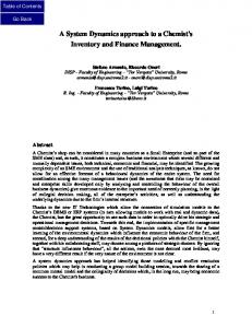
Fig. 1 demonstrates a generic risk management model for information systems. The basic variables (with a very straightforward meaning) are asset value (AV), threat probability (TP), risk (R), safeguards investments (SI), current asset vulnerability (CAV), and months of exposure period (MOE). These variables form two balancing
Using a descriptive, qualitative approach significantly eases risk management processes. ISSN: 1790-0832
176
Issue 2, Volume 5, February 2008
WSEAS TRANSACTIONS on INFORMATION SCIENCE & APPLICATIONS
Denis Trček
investments. But usually the implementation of countermeasures is also delayed due to human factor perception and by organizational issues.
loops that are powered by threats through threat probability - R, SI, MOE and R, SI, CAV are these two balancing loops. Threats are generators in the background of each and every risk management process and their treatment is based on their probabilities. In our case this probability states the likelihood that a threat interacts with a particular resource during a certain one-month period. There are additional variables that serve for proper dimensioning, scaling, and translation, i.e. for tuning the model to a concrete environment that is being simulated: • •
•
•
•
Amortization rate (AR) denotes the rate at which a certain asset’s value is diminishing. Initial asset vulnerability denotes (IAV) vulnerability at the time, when an asset is being put in place for the first time - when new vulnerabilities are discovered, they are prevented by e.g. applying patches to software, which is denoted by vulnerability neutralization value (VNV). Default exposure value (DEV) denotes estimated exposure of an asset before it gets in contact with threats, and after taking appropriate steps this exposure may be diminished, which is modeled by compensation factor (CF). Exposure compensation trigger (ECT) serves as a binary switch to turn on or off the upper loop in order to enable easier calibration of the model, and to easier analyze (in steps) the whole system. Therefore if ECT is set to 0, then the default DEV is taken, which is 0. If ECT is set to 1, the CF gets involved, meaning that the larger the investment in safeguards, the lower the exposure to threats (and vice versa). Acceptable risk value (ARV) is the risk threshold level that is set by security policy (threats below this level are neglected), and actual investments in safeguards are always subject to information delays, which is denoted by delay (D).
Fig. 1: Causal loop diagram of risk management Last but not least, there is one important fact that is also explicitly presented in our generic model. This is residual risk (RR). Very often, risk cannot be completely eliminated, or some risk may be intentionally taken into account, and this is what residual risk is about.
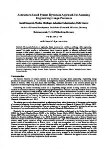
4. Simulations In order to demonstrate an application of this model, only two basic simulations will be presented due to limited space. Both are taking 24 months with simulation increment being set to 0.03125 month. The initial value of an asset is 100, while initial values of other variables are as follows: DEV = VNV = D = 0, AV = ARV = TP = 0.1, and CF = IAV = 1. The simulation results of this basic set up are given in Fig. 2. It can be seen that variables AV, RI, SI and CAV exhibit expected behavior, which is dictated by a naturally diminishing value (amortization) of the asset, assumed to be 10% per month. Now changing only one variable, VNV from 0 to 0.1, 0.2 and further, one very interesting property appears. R, RR, SI and CAV start to oscillate (this is presented in Fig. 3 and Fig. 4).
A few additional words about the delay - it denotes the time between the point when risk becomes constituted and that when safeguards are implemented. It is also assumed that this is the only delay in the whole system that influences safeguard ISSN: 1790-0832
177
Issue 2, Volume 5, February 2008
WSEAS TRANSACTIONS on INFORMATION SCIENCE & APPLICATIONS
Denis Trček
However, this accumulator contributes to the both loops only with its output; so again, it cannot be the source of delays and consequently oscillations. This can be easily checked by setting AV to 1, which means that AV is not diminishing with the time. And indeed, oscillations remain visible.
Fig. 2: Results of the first simulation run with (x-axis presents months, AV is scaled for clarity) Now turning the switch variable on (ECT), which activates the upper, exposure to threats addressing loop, the amplitude of oscillations is enlarged. This implies that this loop must include the cause of oscillations, which is indeed the case – inclusion of the upper loop (exposure to threats loop) increases the values of basic variables in this loop. By changing only CF, the amplitude of oscillations is affected, therefore this variable, as expected, is not the cause of oscillations.
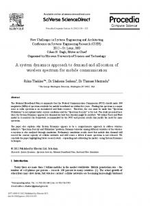
Fig. 4: Results of the second simulation run (R and AV are scaled because of clarity) Further analysis reveals that the reason for these initial oscillations is the way in which the model is initialized. In the lower, stabilizing loop, the oscillation simulation starts with IAV=1 that defines CAV in the first simulation (it is set to 1). However, in the second step, VNV is starting to influence CAV that immediately drops to 0. Consequently, R was overestimated in the first step so it is immediately over-reduced in the second step to compensate that overestimated value from the first step. And this is the source of the initial oscillations – although they are related to model and not the system itself, the lesson is worth remembering. Changes in such systems should be applied gradually and sufficient time should be taken into account for these changes to settle. Now by enlarging the delay D in (which was set to 0 until now), oscillations become easier to analyze. It turns out that these oscillations preserve their amplitude, but their period is enlarged. Further, their shape is exhibiting a large number of higher harmonic components (see Fig. 5).
Fig. 3: The simulation setting that serves for the analysis of oscillations But this is an interesting case – one would expect that D is the source of this oscillations. However, its value is set to 0, so the initial oscillations must be a result of some other variable. Another suspicious candidate is AV, because all accumulators induce delays between inputs and outputs.
ISSN: 1790-0832
This is an important issue for further analysis – the system that this model is representing should be almost instantly reacting to any change. But the reality is that the model is over-reactive, therefore one accumulator in the lower stabilizing loop should be identified. Indeed, R is accumulator by its very nature and will be taken into account as
178
Issue 2, Volume 5, February 2008
WSEAS TRANSACTIONS on INFORMATION SCIENCE & APPLICATIONS
Denis Trček
quantitative treatment, together with simulations, by use of system dynamics.
such during further research and development of the reference IS risk management model.
System dynamics can provide useful insights into risk management dynamics. And being integrated properly into existing information systems and tied to threats through e.g. automatic data exchange about threats with relevant sources like CERTs, a real time decision supporting environment can be build to improve security related decision making. Last but not least, through the analysis of the model better understanding of the modeled phenomenon emerged that gives additional basis for improved decision making. Fig. 5: The third simulation setting that serves for the analysis of oscillations (VNV=0.9 and D=0.6)
References:
The above facts provide the basis for future research to improve decision making processes with regard to risk management. Future research should certainly also focus on another loop that is intentionally left out in this paper, and this is the loop that appears with linking SI and TP. This latter variable is very hard to address but, for completeness of the problem it will have to included, at least with estimated values. Last but not least, human perception will have to be included in the model.
[1] COBIT Steering Committee, COBIT Overview, Information Systems Audit and Control Foundation, Rolling Meadows, 1998. [2] Forrester J., Industrial Dynamics. MIT Press, Cambridge, 1961. [3] Gerber M., Von Solms R., Management of risk in the information age, Computers & Security, Vol. 24, No. 1, 2005, pp. 16-30. [4] Gonzalez J.J., Sawicka A., A Framework for Human Factors in Information Security, Proceedings of the WSEAS Conference on Security, HW/SW Codesign, E-Commerce and Computer Networks, Rio de Janeiro, 2002. [5] Gonzalez J.J. (editor), From Modeling to Managing Security - A System Dynamics Approach, Höyskole Forlaget AS, Kristiansand, 2003. [6] International Standards Organization, Information Processing Systems - Open Systems Interconnection - Basic Reference Model, Security Architecture, part 2, ISO Standard 7498-2, Geneva, 1989. [7] International Standards Organization, IT – Guidelines for the Management of IT Security. ISO / IEC TR 13335-3, Geneva, 1998. [8] International Standards Organization, IT - Code of Practice for Information Security Management, ISO 17799, Geneva, 2000. [8] Trček, D., Managing information systems security and privacy, Springer, Heidelberg / New York, 2006. [10] Von Solms B., Information Security governance: COBIT or ISO 17799 or both? Computers & Security, Vol. 24, No. 2, 2005, pp. 99-104.
5. Conclusions The core process in information systems security is risk management. But intensive networking, numerous existing and emerging services, and exponentially increasing data that present one of the core assets of each organization have caused increasing complexity of these systems. Therefore traditional techniques for risk management are no longer sufficient. There are many disadvantages of those techniques, some of the most important being lack of visibility of relationships between all related elements (i.e. lack of holistic graphical causal presentation), and lack of visible dynamics. Traditional techniques are not really suitable for simulations to anticipate future trends as well. This limits their use to improve decision making for information systems security. To overcome these problems, a new generic risk management model has been developed that identifies information systems security related elements and their relationships. It further enables
ISSN: 1790-0832
179
Issue 2, Volume 5, February 2008
WSEAS TRANSACTIONS on INFORMATION SCIENCE & APPLICATIONS
Denis Trček
Appendix
(14)
risk = IF THEN ELSE(months of exposure = 0, current asset vulnerability * asset value * threat probability, current asset vulnerability * asset value * threat probability * ((1 - threat probability) ^ (months of exposure - 1))) Units: euro
(15)
safeguards investment = DELAY FIXED(risk * acceptable risk value, delay, 0) Units: euro
(16)
SAVEPER = TIME STEP Units: Month
This appendix gives the complete list of equations used for the simulation model (they are given in format suitable for use in VensimTM simulating environment). (01)
acceptable risk value = 0.1 Units: Dmnl [0,1,0.1]
(02)
amortization rate = 0.1 Units: 1/Month
(03)
asset value = INTEG (-asset value * amortization rate, 100) Units: euro
(04)
compensation factor = 1 Units: 1/euro [0,1,0.1]
(17)
threat probability = 0.1 Units: Dmnl [0,1,0.1]
(05)
current asset vulnerability = IF THEN ELSE((initial asset vulnerabilitysafeguards investment * vulnerability neutralization value ) > = 0 , initial asset vulnerability-safeguards investment * vulnerability neutralization value, 0) Units: Dmnl
(18)
TIME STEP = 0.015625 Units: Month
(19)
vulnerability neutralization value = 0 Units: 1/euro [0,1,0.1]
(06)
default exposure value = 0 Units: Dmnl [0,24,1]
(07)
delay = 0 Units: Month [0,24,0.1]
(08)
exposure compensation trigger = 0 Units: Dmnl [0,1,1]
(09)
FINAL TIME = 24 Units: Month
(10)
initial asset vulnerability = 1 Units: Dmnl [0,1,0.1]
(11)
INITIAL TIME = 0 Units: Month
(12)
months of exposure = IF THEN ELSE(exposure compensation trigger = 0, default exposure value, safeguards investment * compensation factor * 10) Units: Dmnl
(13)
residual risk = risk-safeguards investment Units: euro
ISSN: 1790-0832
180
Issue 2, Volume 5, February 2008