System dynamics modeling for renewable energy and CO2 emissions: A case study of Ecuador A. Robalino-L´opeza,b , A. Mena-Nietob , J.E. Garc´ıa-Ramosa,∗ a
b
Department of Applied Physics, University of Huelva, 21071 Huelva, Spain Department of Engineering Design and Projects, University of Huelva, 21071 Huelva, Spain
Abstract It is clear that renewable energy plays a crucial role in achieving a reduction of greenhouse gas emissions. This paper presents a model approach of CO2 emissions in Ecuador in the upcoming years, up to 2020. The main goal of this work is to study in detail the way the changes in the energy matrix and in the Gross Domestic Product (GDP) will affect the CO2 emissions of the country. In particular, we will pay special attention to the effect of a reduction of the share of fossil energy, as well as of an improvement in the efficiency of the fossil energy use. We have developed a system dynamics model based on a relationship, which is a variation of the Kaya identity, and on a GDP that depends on renewable energy, which introduces a feedback mechanism in the model. The main conclusion is that it is possible to control the CO2 emissions even under a scenario of continuous increase of the GDP, if it is combined with an increase of the use of renewable energy, with an improvement of the productive sectoral structure and with the use of a more efficient fossil fuel technology. This study offers useful lessons for developing countries, and it could be used as a policy-making tool because it is easily transferable to any other time period or region. Keywords: CO2 emissions, System Dynamics, Kaya identity, Ecuador
1. Introduction Globally, CO2 is by far the main contributor to anthropogenic greenhouse gas (GHG) emissions (IPCC, 2007, Fig. 2.1): CO2 represents 76.7% Corresponding author: Tel. +34959219791, Fax: +34959219777 Email addresses:
[email protected] (A. Preprint submitted to Energy for Sustainable Development ∗
Robalino-L´ opez), February 5, 2014
of the GHG emissions (approximately 56.6% is from fossil fuels, 17.3% from deforestation, and 2.8% from other sources). Ecuador has a relatively low level of CO2 emissions (2.1 tonnes per capita per year) while Qatar, the world’s largest CO2 emitter per capita in 2009, emitted 44 tonnes per capita. At the same time Venezuela, the largest CO2 emitter in Latin America (LA), emitted annually 6.5 tonnes per capita (World Bank, 2011). It is expected that social and economic development in the coming years could significantly increase Ecuador’s emissions. Observations show that global CO2 emissions, far from stabilizing, have experienced significant growth in recent years. Several international organizations, notably, the Intergovernmental Panel on Climate Change (IPCC), are warning about the need of stabilizing the CO2 and others anthropogenic GHG emissions in order to avoid a catastrophic warming of the climatic system during this century (IPCC, 2007). The IPCC has developed several methods to estimate GHG emissions, such as the Reference Method 1 (IPCC, 2006), which is a top-down technique that uses data from the country’s energy supply (mainly from the burning of fossil fuels), land use, and deforestation rate, among others, to calculate CO2 emissions. It is a straightforward method that can be applied on the basis of the available energy supply statistics (IPCC, 2006). However, the problem arises when it is necessary to conduct more detailed studies and find the driving forces that are behind the emissions, but the data is not available or is not sufficiently disaggregated. In Fig. 1 Ecuador CO2 emissions for the period 1980 − 2010 are depicted (World Bank, 2011)2 . These data only correspond to energy CO2 emissions and do not include the contribution from deforestation. Clearly, one observes an increasing trend which is related with the growth of economic activity. This growth is due to greater prosperity of the inhabitants and to an increase of the population. There are multiple factors that influence the level of CO2 emissions, such as economic development, population growth, technological change, resource endowments, institutional structures, transport models, lifestyles, and international trade (Alc´antara and Padilla, 2005). The identification of the kind of sources of CO2 emissions and of its magnitude is essential information for economic planning and decision makers.
[email protected] (A. Mena-Nieto ),
[email protected] (J.E. Garc´ıa-Ramos ) 1 http://www.ipcc-nggip.iges.or.jp/public/2006gl/pdf/2_Volume2/ V2_6_Ch6_Reference_Approach.pdf 2 http://data.worldbank.org/country/ecuador
2
Figure 1: Ecuador CO2 emissions (1980-2010). CO2 emissions are given in million tonnes of CO2 .
Therefore, this work tries to study the driving forces of CO2 emissions of a given country, particularized to the case of Ecuador, considering doubling the GDP within 10 years, which will approximately correspond to achieve the estimated international average GDP per capita for 2020 (around 12, 000 USD, own estimates based on World Bank data3 ). In this work the increase of the income will be induced through a process of industrialization of the country (see Section 2.7). Unfortunately, this economic growth, according to the environmental Kuznets curve (EKC), in a first stage will also increase the CO2 emissions of the country (Pasten and Figueroa, 2012). Within the EKC hypothesis the relationship between income per capita and some types of pollution is approximately an inverted U. This behavior states that as the GDP per capita grows, environmental damage increases, reaches a 3 GDP given in constant 2005 PPP (purchasing power parity) international dollars (USD). Data taken from http://data.worldbank.org/indicator/NY.GDP.PCAP.PP.KD
3
maximum, and then declines. The Ecuadorian government has, among its goals, the development of strategies to guarantee the energy supply, increase energy cost efficiency, and last, but not least, to minimize the negative impact of economic development on the environment (Mosquera, 2008). Renewable energy sources could play an important role in the diversification of the energy matrix in Ecuador. In particular, CONELEC-004/11 regulation (CONELEC, 2011) establishes the conditions for selling electricity to the national grid, which is encouraging new projects. Below we summarize projects that will increase the use of renewable energy in Ecuador in the upcoming years. 1. Bioenergy. Ecuador has about 71, 000 ha (2009) of sugarcane mostly concentrated in the Coastal Region, near Guayaquil (MAG, 2011). A fuel ethanol pilot program has been planned in Guayaquil and Quito, initially consisting of 5% ethanol blend with gasoline (MRNRE, 2012). If successful, this could set the ground for a nation-wide ethanol fuel program. The use of this kind of fuel will generate savings of about 32 million USD a year, as the country would stop importing about 320, 000 barrels of high octane naphtha4 (15%) (MRNRE, 2012). On the other hand, the total area planted with African palm in Ecuador is 240, 000 ha, with about 200, 000 ha currently being harvested (MAG, 2011). Ecuador could potentially plant up to 760, 000 ha of African palm according to Ecuador’s Association of African Palm Growers (ANCUPA, 2013). Based on projections from the sector in terms of production, domestic consumption and export surplus of red oil, the surplus could grow significantly and reach more than 850, 000 tonnes of red oil in 2025 (USDA, 2011). 2. Hydroelectricity. In 2011 Ecuador had 2, 215 MW of installed hydropower capacity and another 2, 756 MW under construction (CONELEC, 2013). The biggest hydroelectric project is called Coca Codo Sinclair and has a capacity of 1,500 MW and an estimated cost of 2, 245 million USD (the overall project progress is 27.4% up to November 2012). Other hydroelectric projects are: Deisitanisagua with 115 MW, Maduriacu with 60 MW, Mazar Dudas with 21 MW, Minas de San Francisco with 270 MW, Quijos with 50 MW, Sopladora with 487 MW, and Toachi Pilat´on with 253 MW (MEER, 2013). 4
Naphtha is used primarily as feedstock for producing high octane gasoline.
4
3. Solar energy. Through Rural Electrification and Urban Marginal Funds (Fondos de Electrificaci´on Rural y Urbano Marginal - FERUM), Ecuador initiated in 2004 a program of electrification in the countryside using photo-voltaic (PV) generation units. This program started in zones near the border with Peru and in the Amazonian region. Another program using PV panels is executed in the Galapagos Islands to generate a power of 2.1 MW (MEER, 2013). 4. Wind energy. Programs for using wind energy started in 2004. One of the main programs, promoted by the Ministry of Electricity and Renewable Energy (Ministerio de Electricidad y Energ´ıa Renovable MEER), aims at replacing existing thermal generation plant by wind and PV plants in the Galapagos Islands. With the new facilities, 5.7 MW of wind power (plus 2.1 MW of PV power) will substitute most of the 8.8 MW of the thermal generation installed (MEER, 2013; CONELEC, 2013). Other projects for using wind energy in the Ecuadorian continental region are being carried out by the MEER as the one called Villonaco, located in the province of Loja in the south of the country, with a cost of 41.8 million USD and a power capacity of 16.5 MW. 5. Geothermal energy. The geographical location of Ecuador in one of the zones of largest volcano activity, Andean Mountains, is the reason for having a geothermal potential of 534 MW (CEPAL, 2000), which remains unexploited. The main geothermal project existing in Ecuador (Tufi˜ no-Chiles-Cerro Negro-TCCN Project) is located in the north of the country. Besides, there is a join project with Colombia to install a plant with a capacity of 15 MW (CEPAL, 2000). Other geothermal resources in the center of the country could also be exploited in the future. It is a very complicated task to predict how much the economy will grow in the near future. This growth will strongly modulate the CO2 emissions of any country and therefore it will be crucial to make a realistic estimate of CO2 emissions. On the other hand, the different feedback-mechanisms, both in the climatic and in the economic system make any prediction highly questionable beyond 5−10 years (Fiddaman, 2002). However, it is critical to provide accurate information to policymakers in order to design appropriate energy policies for the near future (Bahrman et al., 2007). This paper explores the relationship between economic growth, productive sectors, energy consumption, changes in the use of renewable energy, 5
improvements in the efficiency of fossil energy, and the CO2 emissions of the country. To estimate the CO2 emissions in the near future we will define different scenarios. The model is based on a variation of the Kaya identity (Kaya and Yokobori, 1993) and on an approach of formation of GDP which includes a contribution from renewable energy (Chien and Hu, 2008). The model has been implemented using the system dynamics (SD) technique (Forrester, 1961) on a Vensim platform (Vensim, 2011). It was originally proposed by J. Forrester to understand how systems change as a function of time (Begueri, 2001). The considered data corresponds to the period 1980 − 2010 and it has been extracted from the official dataset of the Ecuadorian Institute of Statistics and Census (Instituto Nacional de Estad´ıstica y Censos INEC) (INEC, 2012), Central Bank of Ecuador (Banco Central de Ecuador - BCE) (BCE, 2012), World Bank (World Bank, 2011)5 , and International Energy Agency (IEA, 2013). In the rest of this paper GDP-PPP will be referred as GDP, for brevity. The raw data has been processed using a Hodrick-Prescott filter (HP) (Hodrick and Prescott, 1997) which allows to generate a smooth representation of a time series. The Kaya identity is commonly used as an analytical tool to explore the main driving forces that control the amount of carbon dioxide emissions (Alc´antara and Padilla, 2005; Mena-Nieto et al., 2009). According to this identity, CO2 emissions of a given country are broken down into the product of four factors: carbon intensity (defined as the CO2 emitted per unit of energy consumed), energy intensity (defined as the consumed energy per unit of GDP), economic rent (defined as GDP per capita), and population (Fiddaman, 2002). SD is a method for modeling, simulating and analyzing complex systems. A system is defined as a collection of elements in which interactions are modeled as flows between reservoirs in time steps, and in which the rate of change depends on the value of the variables that define the system (feedback mechanisms). Therefore, the main goal of SD is to understand how a given system evolves, and even more importantly, to understand the causes that govern its evolution (Garc´ıa , 2011). The basis of SD has been reanalyzed in detail in (Radzicki and Tauheed, 2009; Tan et al., 2010). The use of SD methodology for the understanding of complex environmental systems has increased significantly. SD has been used to study climate change policies and the evolution of the economy (Fiddaman, 2002; 5
Economic official data set used is given in constant 2005 PPP international dollars.
6
Nordhaus and Yang, 1996; Naill et al., 1992; Feng et al., 2012). Bassi and Baer (2009) carried out an SD study trying to answer whether an annual investment of 1% of GDP to mitigate the negative economic impacts of climate change, would allow for the reduction GHG emissions in Ecuador. The paper is organized as follows: section 2 summarizes the main data indexes of the country and outlines the method used for the case study; section 3 presents and discusses the main results of this work, and lastly, section 4 provides the summary and the conclusions. 2. Study area and methodology 2.1. Overview of the study area Ecuador (officially the Republic of Ecuador) has an area of 272, 046 km2 and a population of more than 14 million (2010) (INEC, 2012). Ecuadorian territory, which includes the Galapagos Islands, 1, 000 km off the west coast, has the planet’s densest biodiversity. This species diversity makes Ecuador one of the 17 mega-diverse countries in the world (ConservationInternational, 2012). The new Ecuadorian constitution of 2008 is the first one in the world to recognize legally enforceable rights of Nature, or ecosystem rights (TCELDF, 2011). Ecuador is a medium-income country with a Human Development Index score of 0.695 (UNDP , 2011) and about 35.1% of its population lives below the poverty threshold (Index Mundi, 2012). Its economy is the eighth largest in Latin America and experienced an average annual growth of 4.6% between 2000 and 2006. The Ecuadorian GDP was multiplied by 2.3 times between 1980 and 2010, and the GDP reached a value of around 104 billion US dollars (2005USD) that year. Note that the country’s public finances are healthy, but they have recognized that the Achilles heel of the Ecuadorian economy is the external sector, due to the deficit, without including oil exports, in the trade balance (BCE, 2012). Since the late 1960’s oil extraction increased. Proven reserves of the country in 2013 are estimated at around 8 billion barrels (IEA, 2013; BCE, 2012). The extreme poverty6 rate has declined significantly between 2000 and 2010. In 2000, the estimate was approximately 20.7% of the population, while by 2010 this number had dropped up to 4.6% of the total population. 6
Population below 1.25 USD a day is the percentage of the population living on less than 1.25 USD a day at 2005 international prices.
7
This is largely explained by emigration and the economic stability achieved after the dollarization of the economy. Poverty rates were higher for indigenous peoples, afro-descendants and rural areas, reaching 44% of the native population (World Bank, 2011). 2.2. Formulation of model The model uses a variation of the Kaya identity, where the amount of CO2 emissions from industry and from other energy uses may be studied quantifying the contributions of five different factors: global industrial activity, industry activity mix, sectoral energy intensity, sectoral energy mix, and CO2 emission factors. Moreover, we consider different sub-categories concerning the industrial sectors and the fuel type. The CO2 emissions can be written as, C=
X ij
Cij =
X ij
Q
X Qi Ei Eij Cij = Q · Si · EIi · Mij · Uij Q Qi Ei Eij ij
(1)
where C is the total CO2 emissions and Cij is the CO2 emissions arising from fuel type j in the productive sector P i; Eij is the consumption of fuel j in the industrial sector i, where E = ij Eij ; the energy matrix is given C E by Mij ( Eiji ) and the CO2 emission factor by Uij ( Eijij ). Note that the index i runs over five productive sectors and the index j over the type of energy sources. The raw data to perform the model correspond to the official available data on Ecuador, provided by the INEC7 , the BCE8 , the World Bank9 , and the International Energy Agency10 . The subsequent data analysis and the preprocessing of the time series was performed using the Hodrick-Prescott (HP) filter (Hodrick and Prescott, 1997), which allows isolation of outliers (economic crises, random behavior of markets, etc) of the time series under study. After that, it is possible to get the trend component of a time series and to perform more adequate estimations. The smoothing parameter λ of the filter, which penalizes acceleration in the trend relative to cycle component, needs to be specified. Most of the business cycle literature use past data and a value of the smoothing parameter λ equal to 100 (Hodrick 7
http://www.inec.gob.ec/estadisticas/, http://www.ecuadorencifras.com/ http://www.bce.fin.ec/indicador.php 9 http://data.worldbank.org/country/ecuador 10 http://www.iea.org/countries/non-membercountries/ecuador/ 8
8
Figure 2: Schematic diagram of the methodology used in the paper.
and Prescott, 1997). Indeed, all time series used in this paper have been computed using the HP filter with a λ value of 100. The simulation period extends from 1980 to 2020, where 1980 − 2010 is used to fix the parameters of the model and 2011 − 2020 corresponds to the forecast period, under the assumption of different scenarios concerning the evolution of the GDP, the evolution of the energy mix, and the efficiency of the used technology in minimizing the CO2 emissions. The geometric growth rate (Rowland, 2003; Jin et al., 2009) has been used to extrapolate the trends into the forecast period. The Seemingly Unrelated Regression (SUR) (Zeller, 1962) in STATA software platform (STATA, 2012) has been used to parameterize the GDP formation. The validation of the model has been done with the mean absolute percentage error (MAPE) and a sensitivity analysis was performed through the Logarithmic Mean Divisia Index (LMDI) (Ang, 2005). Fig. 2 shows in a schematic way how the calculations have been performed using the different techniques described in previous paragraphs.
9
2.3. Economic submodel Much attention has been given recently to the notion of sustainable energy consumption. This work uses a perspective of environmental economics to include the influence of renewable energy usage directly contributing to the formation of the GDP (Domac et al., 2005), which suggests that renewable energy can increase the GDP in two different ways: (i) the business expansion and new employment brought by renewable energy industries result in economic growth; (ii) the import substitution of energy has direct and indirect effects on increasing the GDP and the trade balance. This paper uses the second process to model GDP formation (Chien and Hu, 2008). Following closely to Chien and Hu (2008) we use the expenditure approach to form the GDP GDP = C + I + G + X − M,
(2)
where C is the final household consumption expenditure, I is the gross domestic capital formation, G is the general government final consumption expenditure, X is the export; and M the import. The deduction of imports from exports is the trade balance TB. On the other hand, according to Chien and Hu (2008) the variable G is eliminated from the model estimation to avoid multicollinearity. To avoid the problems of inputting raw data, a rescaling of the smoothed time series has been used so that they are all on approximately the same scale. The system of theoretical GDP formation model is made up by the following equations: GDP I TB Eimp C
= = = = =
a1 · I + a2 · T B + a3 · C + a4 · Eimp + a5 · RN + ǫ1 b1 · RN + b2 · C + ǫ2 c1 · Eimp + c2 · RN + ǫ3 d1 · RN + ǫ4 f1 · Eimp + f2 · T B + ǫ5
(3) (4) (5) (6) (7)
where Eimp is the energy import, RN is the renewable energy and ǫ1 ... ǫ5 are residuals. Note that Eqs. (3)-(7) form our model for the GDP. Coefficients appearing in these equations are determined using the SUR for the datasets of the period 1980 − 2010 and therefore their values are a consequence of the data. In Eq. 3, GDP is influenced by capital formation, trade balance, 10
and consumption. Chien and Hu (2007) suggested that energy inputs may affect GDP, therefore, energy imports and renewable energy are included as well Eq. (3). Note the negative value of a5 in table 1. Table 1: Estimated coefficients for the GDP formation equations (see Eqs. (3)-(7))a .
Variable I
c
TB C
d
e
Eimp RN
g
f
GDP b 1.16∗∗∗ (5.11) 0.99∗∗∗ (3.46) 1.21∗∗∗ (7.70) 0.05∗∗∗ (2.66) −0.50∗∗∗ (-4.44)
I
TB
C -6.07∗∗∗ (-41.44)
0.01∗∗∗ (4.14) 0.04 (0.28)
−0.27∗∗∗ (-100.17)
Eimp
0.50∗∗∗ (100.40)
−0.84∗∗∗ (-5.40)
−36.79∗∗∗ (-5.47)
a
*** represents significance at the 1% level and numbers in the parentheses are tstatistics. Estimation Method: SUR. Sample: 1980-2010. Included observations: 155. b GDP in 1010 USD. c I in 1010 USD. d TB in 1010 USD. e C in 1010 USD. f Eimp in 106 toe. g RN in 106 toe.
In Eq. (4) capital formation is influenced by renewable energy, since theory predicts that increasing the use of renewable energy will result in business expansion and thus capital could be accumulated in long term, but its implementation is expected to have a negative short term effect in GDP (this is confirmed with a negative value of b1 in table 1). In Eq. (5) energy imports and renewable energy influence trade balance (both coefficients, c1 and c2 , have positive values in table 1). The theory proposed by Domac et al. (2005) suggests that the use of renewable energy results in import substitution by domestic-produced renewable energy, and thus trade balance will increase by the use of renewable energy. Furthermore, if 11
renewable energy could cause import substitution, then the imports of energy should be reduced by the increase of renewable energy (in Eq. (6) the value of the coefficient d1 is negative). Although Ecuador is a net exporter of fossil energy, the use of renewable energy can help diversify its energy matrix and reduce emissions. In Eq. (7), according to international trade theories, the domestic price of goods increases as the same kind of goods are exported, while it decreases as the same kind of goods are imported. Thus, trade balance influences consumption through changes in domestic prices. The imports of energy influence domestic energy prices and the consumption of energy. As a result, consumption of energy-related products is also affected. Ecuador exports crude oil and imports refined products, such as diesel and liquid petroleum gas (LPG) which affects the value of TB and Eimp in Eq. (3). The results obtained after the fitting of the smoothed series of data are depicted in table 1. Note that the error terms are correlated through the GDP formation equations, because the variables in Eq. (3) are not fully statistically independent. All the coefficients are individually significant at the 0.01 level except the coefficient between Eimp and TB. According to the results of table 1 renewable energy generates a reduction of GDP and of I in the short term, however they have a positive impact on the TB and a large negative effect on the Eimp . 2.4. Energy consumption and productive sectoral structure submodel Energy consumption refers to the use of primary energy before transformation into any other end-use energy, which is equal to the local production of energy plus imports and stock changes, minus exports and the amount of fuel supplied to ships and aircrafts engaged in international transport. It is given in tonnes of oil equivalent (toe). Energy intensity is defined as the ratio of energy consumption to GDP (World Bank, 2011). In this work we consider five sectors to the productive sectoral structure: 1) agriculture, fishing and mining, 2) industry, 3) construction, 4) services, trade and residential, and 5) transportation. These will be represented inside the model by its contribution to the country’s economy (Si ), by its energy intensity (EIi ) and by their energy mix (Mij ). Index i runs over each sector of the productive sectoral structure and index j runs over each kind of fuel: 1) natural gas, 2) coal, 3) pretroleum, 4) renewable energy, and 5) alternative and nuclear energy. Note that the different economic sectors have different energy intensity (Cancelo and D´ıaz, 2002). The differences in energy intensity between each 12
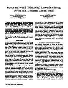
sectors can be explained by two reasons: i) differences in the efficiency of the energy used in each sector and ii) differences in the economic activity of each sector. 2.5. CO2 intensity and energy matrix submodel CO2 intensity (CO2int ) of a given country corresponds to the ratio of CO2 emissions and the total energy written in terms of mass of P consumed P oil equivalent (CO2int = ij Cij / i Ei ). The value of the CO2int in a given year depends on the particular energy mix during that year. The energy matrix is given by Mij , but it is more convenient to sum over the different sectorsP and aggregate the fossil fuel contributions. Therefore, we define P Mj = i Eij / ij Eij , where j = 1 corresponds to natural gas, j = 2 to coal, j = 3 to petroleum, j = 4 to renewable energy, and j = 5 to alternative and nuclear energy. Finally, we define ES1 = M1 + M2 + M3 (share of fossil energy in the total consumption), ES2 = M4 (share of renewable energy), and ES3 = M5 (share of alternative and nuclear energy), besides we introduce ES11 = M1 (share of natural gas), ES12 = M2 (share of coal), ES13 = M3 (share of petroleum). Therefore, ES1 = ES11 +ES12 +ES13 and ES1 + ES2 + ES3 = 100%. In order to simplify the description, in this work we assume that ES2 and ES3 do not contribute to CO2 emissions. Following the methodology recommended by the IPCC, that is, the Reference method (IPCC, 2006), Tier 1 approach for the fossil energy mix has been used. 2.6. Causal diagram of CO2 emissions To understand why and how CO2 emissions change over time, we need to know the factors that separately affect or control CO2 emissions. In particular, it is extremely useful to represent the driving forces of CO2 emissions in a hierarchical way, showing the causality relationship between the different variables. All this information constitutes the causal diagram. In this work the variables that will determine the amount of CO2 emissions are: GDP (formation components), share of the different productive sectors in the GDP, energy intensity of each sector, energy consumption, energy matrix, and carbon dioxide intensity. They are all represented schematically in Fig. 3. It can be observed that the CO2 emitted into the atmosphere has several connections with the variables of the model: economic growth and its different productive activities demand more energy, this increase in energy consumption induces higher CO2 emissions that could be regulated by changes in the energy matrix and in the productive sectoral structure of the country. 13
Figure 3: Model causal diagram: continuous lines stand for the relationship between variables while dashed lines correspond to control terms (S: productive sectoral structure, M: energy matrix, U: emission factors). Bold line represents the feedback mechanism.
It is worth to note the presence of a feedback mechanism associated to the influence of renewable energy on the GDP (see bold line in Fig. 3). 2.7. Scenarios The goals that will be considered to define the different scenarios that will be proposed, under the general purpose of “improve the quality of life of people with the least environmental impact” are: Goal 1, by 2020 the GDP per capita will reach the international average (≈ 12, 000 USD according to our estimates based on World Bank data) through a process of industrialization and improvement of the productive sectoral structure of the country; Goal 2, in regard to the Goal 1, the use of renewable energy will be increased up to almost 25% of the total energy consumption; Goal 3, in regard to Goal 1 and Goal 2, the energy efficiency will be enlarged by a reduction of the energy intensity and by changes in the productive sectoral structure (see below). Taking into account the latter goals, we propose four scenarios concerning the growth of the GDP, the evolution of the energy matrix and of the productive sectoral structure for the period 2011 − 2020. 1. Baseline scenario (BS): the GDP, the energy matrix and the productive sectoral structure will evolve through the smooth trend of the period 1980 − 2010 extrapolated to 2011 − 2020 using the geometric growth rate method. 14
2. Doubling of the GDP (GDPx2 scenario, Goal 1): the GDP (in 2020) will double the one of 2010 and the country will reach the international GDP per capita average that has been estimated to be around 12, 000 USD. To generate this scenario a constant annual growth of the GDP formation components (I, T B, C, Eimp ) of 7% per year between 2011 to 2020 will be assumed and a structural change in the productive sectoral structure will be implemented through a growth of 1% per year in the share (Si ) in the GDP of sectors with more profit to the country economy: industry sector (sector 2) and service, trade, and residential sector (sector 4). The rest of the variables will evolve as in the BS scenario. 3. Doubling of the GDP and of the share of renewable energy (GDPx2+GE scenario, Goal 2): the doubling of the GDP and the change of the productive sectoral structure as in the GDPx2 scenario is considered, however the share of fossil energy, ES1 , will be reduced approximately one point per year, passing from a 88% in 2011 to a 76% in 2020 due to a constant annual growth of the renewable and alternative energy share (ES2 and ES3 ). This goal is realistic considering the state of development and evolution of the energy technology and of the various energy projects implemented by the Ecuadorian government as stated in Mosquera (2008). 4. Doubling of the GDP, doubling of the renewable energy share and improvement in the efficiency of the energy use (GDPx2+GE+EF scenario, Goal 3): the doubling of the GDP, the change in the productive sectoral structure and the change of the share of ES1 is the same than in the GDPx2+GE scenario. Moreover, an improvement in the efficiency of the energy use is implemented with a 1% reduction of the energy intensity in the industry sector (sector 2), in the trade, service and residential sector (sector 4) and in the transportation sector (sector 5). This goal, as that of the third scenario, is consistent with the energy policy of the Ecuadorian government (Mosquera, 2008). In the BS scenario a big change does not exist in the evolution of energy consumption or in the environmental goals, therefore the country follows the trend of the period 1980 − 2010. The GDPx2 scenario clearly corresponds to a situation where the economy is growing rapidly and no mitigation measurements to reduce the CO2 emissions are carried out. In the third scenario, GDPx2+GE, the growth of the economy is combined with a goal 15
of reduction of the share of ES1 in the energy matrix. Besides the use of renewable energy, in the fourth scenario, GDPx2+GE+EF, an improvement in the energetic efficiency of the productive sectors is implemented, which helps to reduce the CO2 emissions. It is important to note that for both, economy and energy, the goal of this paper is not to perform a rigorous forecast of the GDP, energy consumption and energy intensity, however, we try to establish a baseline and also other reasonable scenarios that could be useful as reference points for policy makers or further studies. 2.8. Model validation and verification Official dataset from 1980 to 2010 and the output of the model can be compared to test the predictive power and robustness of the model. This analysis can be carried out calculating the mean absolute percentage error (MAPE), which is defined as, 1 X At − F t MAPE(%) = (8) At × 100, n where, At, Ft, and n are the real data, the calculated values, and the number of data, respectively. Table 2: Mean absolute percentage error (MAPE) for selected variables.
VARIABLE GDP Energy consumption CO2 intensity CO2 emission
MAPE(%) 2.22 3.42 15.28 15.96
In table 2 the corresponding MAPE values for some selected variables are given. These results indicate the robustness of the model. Note that in this paper we consider that CO2 emissions come only from the burning of fossil fuels and we do not include the contribution coming from the production of cement, because the lack of official data. Therefore, our projections will consider CO2 emissions only. This fact, together with the process of smoothing (HP filter) of the raw dataset and the use of general emission factors (IPCC, 2006) justify the somehow large deviations observed in table 2 for the CO2 intensity and CO2 emissions. 16
3. Results and discussion This section includes the main results of this work, which is the estimation of CO2 emissions for the studied scenarios. For completeness, some other projection that, indeed, correspond to the definition of the different scenarios are also shown. 3.1. GDP and GDP per capita The value of the GDP for the two types of considered scenarios (BS and GDPx2) is presented in Fig. 4, where one can see that the estimated GDP for the GDPx2 scenario will be around 196 billion USD in 2020 (37% higher than for BS scenario). Note that the projected GDP is not a forecast but a consequence of the considered scenarios. Assuming an annual increase of the population of 1.2%, the population will pass from 14.5 million in 2010 to 16.5 million in 2020, thus the GDP per capita in 2020 will be around 12, 000 USD (which is roughly the prevision that has been considerate for the international average of GDP per capita). In the GDPx2+GE and GDPx2+GE+EF scenarios, the GDP would be lower with respect to the GDPx2 scenario with a reduction of about 10 billion USD in 2020 due to the promotion of renewable energy. The connection between GDP and renewable energy is obtained through the feedback mechanism of the model. In the GDPx2+GE+EF scenario the reduction in the GDP in slightly smaller (about 8 billion USD) because of the improvement in the energy intensity. Note that the tiny deviations between the different GDPx2 scenarios are due to the feedback mechanism between GDP and renewable energy. 3.2. Energy consumption Energy consumption is calculated through the product of the energy intensity of each productive sector (EIi ) and the corresponding share of the GDP (Si ) of every sector. The values of the energy consumption for the period 2011 − 2020 are represented in Fig. 5. In 2020 the BS scenario generates a demand of 16.4 million toe, the GDPx2 scenario about 24.6 million toe (45% higher than the BS scenario), and the GDPx2+GE scenario generates a demand of 23.4 million toe (38% higher than the BS scenario). These two last scenarios show the growth of the energy consumption due to the increase of the GDP and to the changes of the productive sectoral structure. Finally, the GDP2+GE+EF scenario generates a demand of 20.5 million toe (only 21% higher than in the BS scenario). It clearly shows the benefits of the reduction of the energy intensity. 17
Figure 4: Ecuador GDP for the period 2011 − 2020. Green line corresponds to the BS scenario, purple line to the GDPx2 scenario, blue line to the GDPx2+GE scenario, and orange line to the GDPx2+GE+EF scenario.
The estimated values of energy consumption in each productive sector in 2020 are shown in table 3 to illustrate the differences between sectors. 3.3. Energy matrix and CO2 intensity Two types of evolution of the energy matrix have been taken into account in the calculations, in particular, for the share of fossil energy, ES1 , and its components (ES11 , ES12 , and ES13 ). In the first case, the evolution of ES1 follows the tendency of the period 1980 − 2010. In the second case, a continuous drop of ES1 up to 76% in 2020 due to the doubling of the renewable energy share is assumed. Besides, changes in the fuel use of the productive sectoral structure have been carried out, which suppose a reduction of the energy intensity. A very important result is that the reduction of the global CO2int is twofold, on one hand, it is due to the use of a more efficient fossil fuel technology (lower CO2 intensity) and, on the other hand, due to the reduction of the ES1 share to the energy matrix. Both contributions are equally important. Note that the 2011 − 2020 period presents a reduction 18
Figure 5: Ecuador energy consumption for the period 2011−2020. Green line corresponds to the BS scenario, purple line to the GDPx2 scenario, blue line to the GDPx2+GE scenario, and orange line to the GDPx2+GE+EF scenario.
of the global CO2int from 2.7 tCO2 /toe in BS scenario to 2.3 tCO2 /toe in GDPx2+GE+EF scenario. The energy matrix and the CO2 intensity are shown in table 4. 3.4. CO2 emission This section includes the main outcome of this work, based on the different scenarios. Fig. 6 shows the CO2 emissions as a function of time for the period 2011 − 2020, under the four considered scenarios. In 2020 the highest CO2 emission corresponds to the GDPx2 scenario, while the lowest corresponds to the BS scenario. The GDPx2+GE and GDPx2+GE+EF scenarios, which imply the continuous growth of the GDP and the application of attenuation measures, with a reduction of the fossil energy contribution to the energy matrix and changes in the productive sectoral structure, present a clear reduction of CO2 emissions with respect to the GDPx2 scenario. In particular, in 2020 the CO2 emissions would reach 66 million tonnes of CO2 in the GDPx2 scenario, and only 45 million tonnes of CO2 in the BS 19
Table 3: Energy consumption in ktoe by productive sector in 2020.
Scenario BS GDPx2 GDPx2+GE GDPx2+GE+EF
Sector 1 96 105 99 101
Sector 2 3740 5648 5354 4729
Sector 3 92 126 119 121
Sector 4 3385 5539 5250 4885
Sector 5 9626 13225 12537 10642
Table 4: Energy matrix (in %) and CO2 intensity (in tCO2 /toe).
2010 ES11 ES12 ES13 ES2 +ES3 CO2 intensity
0.65% 0% 87.42% 11.92% 2.68
2020 (BS, GDPx2) 0.66% 0% 87.26% 12.09% 2.67
2020 (GDPx2+GE, GDPx2+GE+EF) 0.66% 0% 75.89% 23.46% 2.33
scenario. With the application of a reduction of ES1 , up to 76% in the GDPx2+GE scenario, without modifying the energy intensity, one reaches the value of 54 million tonnes of CO2 , while implementing energy efficiency measures in the productive sectoral structure (GDPx2+GE+EF scenario) the emissions are reduced up to 48 million tonnes of CO2 . The BS scenario indicates a 1.5-fold increase in the CO2 emissions in 2020, relative to the year 2010, while the GDPx2 scenario gives rise to an increase of 2.1 times. This implies that the amount of CO2 emissions in the GDPx2 scenario during 2011 − 2020 will be 96 million tonnes of CO2 higher than in the BS scenario. Scenarios where renewable energy and efficiency goals are implemented show that it is possible to increase the GDP in a constant way, mitigating, at the same time, the CO2 emissions, therefore reducing the rise of the emissions due to the higher economic activity. In particular, the most efficient scenario GDP2+GE+EF provides a remarkable reduction. In 2020 the CO2 emissions will be 16.5% lower than in the GDPx2 scenario. Furthermore, the GDP2+GE scenario generates 49 million tonnes of CO2 more than BS scenario during the 2011 − 2020 20
Figure 6: Ecuador CO2 emissions for the period 2011 − 2020. Green line corresponds to the BS scenario, purple line to the GDPx2 scenario, blue line to the GDPx2+GE scenario, and orange line to the GDPx2+GE+EF scenario.
period, which supposes a reduction of 47 million tonnes of CO2 with respect to the GDPx2 scenario. Finally, the GDP2+GE+EF scenario generates 16 million tonnes of CO2 more than BS scenario during the same period, which supposes a large reduction of 80 million tonnes of CO2 with respect to the GDPx2 scenario. For further detail see table 5. 3.5. Sensitivity analysis In this section we will carry out a sensitivity analysis based on the LMDI (Ang, 2005). This analysis will allow us to determine the relative importance of each term conforming the CO2 emission formula (1). Indeed, it is very enlightening to write down the increase on CO2 emission relative to the value of a given period, and to decompose it as the product of the factors corresponding to the different driving forces that conform the CO2 emission. Therefore we can write (Ang, 2005), Dtot = Dact × Dstr × Dint × Dmix × Demf 21
(9)
Table 5: CO2 emissions for the 2011 − 2020 period in the different scenarios. Emissions are given million tonnes of CO2 .
Scenario BS GDPx2 GDPx2+GE GDPx2+GE+EF
Emissions
Emissions (2020)
Emissions (2020)/ Emissions (2010)
(2011-2020)
Emissions (2011-2020)/ EmissionsBS (2011-2020)
45.33 65.79 54.44 47.72
1.43 2.08 1.72 1.51
389.40 485.68 438.72 405.42
1.00 1.25 1.13 1.04
where Dtot is the CO2 emission (relative to the year 2010), Dact is the GDP term, Dstr is the structure term (the share of the different sectors to the GDP), Dint the energy intensity term, Dmix the energy mixing term, and Demf the emission factor term. Note that because the emission factors, given by the IPCC, do not change over the time, Demf = 1 all the time and therefore it will not be shown in the tables. Table 6: Results of the CO2 emission decomposition factors for the period 2010-2020.
Scenario BS GDPx2 GDPx2+GE GDPx2+GE+EF
Dtot 1.43 2.08 1.72 1.51
Dact 1.38 1.89 1.79 1.82
Dstr 1.00 1.06 1.06 1.06
Dint 1.04 1.04 1.04 0.90
Dmix 1.00 1.00 0.87 0.87
The LMDI analysis shows that by 2020 in the BS scenario the CO2 emissions increase 43% (Dtot = 1.43), due to the increase of the GDP in 38% and to the increase of the energy intensity term in 4%, while the rest of terms remain invariant. The GDPx2 scenario presents CO2 emissions that are more than the double that in 2010. This increase is due to a growth of 89% of the GDP, 6% of the structure term, and 4% of the energy intensity term. The GDPx2+GE scenario only presents an increase of 72% in the emissions. In this case, the GDP growths 79%, the structure term 6%, and the intensity term 4%, while the mixing term reduces 13%. Finally, in the GDPx2+GE+EF scenario the emissions only increase 51%: the GDP term growths 82%, the structure term 6%, while the energy intensity term 22
reduces 10% and the mixing term 13%. All the coefficients are summarized in table 6 and in a pictorial way in Fig. 7. In this figure five axes are depicted corresponding to the five columns appearing in table 6. The value of the vertical axis, Dtot , corresponds to the product of the four remaining variables, Dact , Dstr , Dint , and Dmix .
Figure 7: Pictorial view of the CO2 emission decomposition factors for the period 20102020.
4. Summary and conclusions This paper presents a model based on a variation of the Kaya Identity and on an approach of GDP formation which is supported with the use of renewable energy. The case study is Ecuador and covers the period 1980−2020. The official data set (1980−2010) was used to parameterize the model, while with the second part of the period (2011 − 2020) an estimation of different variables, including the CO2 emissions, was carried out. To this end, the GDP and the energy intensity have been modeled. Moreover, different scenarios that present the evolution of the energy matrix and the productive sectoral structure have been defined. 23
First, a BS scenario (baseline scenario) has been defined, in which the variables of the model were parameterized according to the observed tendency during the period 1980 − 2010, assuming a geometric growth rate during the period 2011 − 2020. The second scenario, called GDP2, is characterized by the doubling (relative to 2010) of the GDP during the period 2011 − 2020 (with the goal of reaching the estimated international average GDP per capita in 2020). In the third scenario, called GDP2+GE scenario, besides assuming the doubling of the GDP, we impose the decreasing of the fossil energy share (ES1 ) up to 76%. Finally, in the fourth one, GDP2+GE+EF scenario, we complement the GDP2+GE scenario including changes in the productive sectoral structure to achieve a reduction of energy intensity, which supposes a lower CO2 intensity. The main outcome of this work is the estimate CO2 emissions in 2020 in each scenario. In the BS scenario this value amounts to 45 million tonnes, in the GDPx2 scenario it corresponds to 66 million tonnes, in GDPx2+GE scenario to 54 million tonnes of CO2 , and in the GDPx2+GE+FE scenario to 48 million tonnes of CO2 . Note that the BS scenario corresponds to a modest GDP increase, while in the others the GDP increases heavily. The highest emissions are for the GDPx2 scenario where no mitigation measures are taken. The other two scenarios show us that it is possible a sizable reduction of the emissions, promoting the renewable energy (GDPx2+GE scenario) and on top of that modifying the productive sectoral structure, therefore, reducing the energy and the CO2 intensities, as in the GDPx2+GE+EF scenario. It is worth to note that both promotion of renewable energy and improvement of the energy intensity are equally effective attenuating CO2 emissions. The methodology presented in this paper is useful to estimate the CO2 emissions of a given country and to understand the driving forces that guide this process, such as economic growth, energy use, energy mix structure, and fuel use in the productive sectors. This methodology is easily transferable to other countries, regions, and time periods. Moreover, it can be very useful as a pedagogical tool for explaining to policymakers the possible ways to design a policy for reducing CO2 emissions in a medium term horizon. Note that in the present status of the model we consider a feedback mechanism between the GDP and the energy consumption through the influence of the renewable energy.
24
5. Acknowledgment This work has been supported by the Spanish Ministerio de Econom´ıa y Competitividad and the European regional development fund (FEDER) under project number FIS2011-28738-C02-02, by Junta de Andaluc´ıa under project P07-FQM-02962, and by Spanish Consolider-Ingenio 2010 (CPANCSD2007-00042). One of the authors (ARL) gives special thanks to the SENESCYT (Ecuador) and the AUIP (Spain) for the institutional and financial support. References Alc´ antara, V., Padilla, E., 2005. “Analysis of CO2 and its explanatory factors in the different areas of the world”. Technical Report. Universidad Autonoma de Barcelona, Department of Economics Applied, Spain. ANCUPA, 2013. “Area National Oil Palm”, Ecuador Association of African Palm Growers (Asociaci´ on Nacional de Cultivadores de Palma Africana del Ecuador). http://www.ancupa.com. Ang, B.W., 2005. “The LMDI approach to decomposition analysis: a practical guide”. Energy Policy 33, 867-871. Bahrman, S., Lenker, C., Michalek, J., 2007. “A model-based approach to analyze the effects of automotive air emissions policy on consumers, producers, and air quality”. Eco Design and Manufacturing. Bassi, A., Baer, A., 2009. “Quantifying cross-sectoral impacts of investments in climate change mitigation in Ecuador”. Energy for Sustainable Development 13, 116-123. BCE-Central Bank of Ecuador (Banco Central de Ecuador), 2012. “BCE indicators homepage”. http://www.bce.fin.ec/indicador.php. Begueri, G., 2001. “System Dynamics: A New Approach”. Technical Report. Universidad Nacional de San Juan, Argentina. Cancelo, M., D´ıaz, M., 2002. “CO2 emissions and economic growth in EU countries”. Journal of International Development Economic Research. Technical Report. Universidad de Santiago de Compostela, Spain. JEL classification: O13, O14, O52. CEPAL, Comisi´ on Econ´omica para Am´erica Latina y el Caribe, 2000. “PROYECTO OLADE/CEPAL/GTZ: Estudio para la Evaluaci´ on del Entorno del Proyecto Geot´ermico Binacional ”Tufi˜ no-Chiles-Cerro Negro, LC/R. 1995, 23 de junio de 2000”. Chien, Taichen, Hu, Jin-Li, 2007. “Renewable energy and macroeconomic efficiency of OECD and non-OECD economies”. Energy Policy 35, 3606-3615. Chien, Taichen, Hu, Jin-Li, 2008. “Renewable energy: An efficient mechanism to improve GDP ”. Energy Policy 36, 3045-3052. CONELEC11, National Council for Electrification (Consejo Nacional de Electrificaci´on), 2011. “Treatment for energy produced from non-conventional renewable energy resources (CONELEC Regulation No. 004/11)”. http://www.conelec.gob.ec. CONELEC13, National Council for Electrification (Consejo Nacional de Electrificaci´on), 2013. http://www.conelec.gob.ec. Conservation-International, 2012. “Megadiversity: The 17 biodiversity Superstars”. http://www.conservation.org/documentaries/Pages/ megadiversity.aspx.
25
Domac, J., Richards, K.,Sarafidis, S., 2005. “Socio-economic drivers in implementing bioenergy projects”. Biomass and Bioenergy 28, 97106. Feng, Y.Y., Chen, S.Q., Zhang, L.X. 2012. “System dynamics modeling for urban energy consumption and C02 emissions: A case study of Beijin, China”. Ecological Modelling, in press. Feng, Y.Y., Zhang, L.X., 2012. “Scenario analysis of urban energy saving and carbon emission reduction policies: a case study of Beijing” Resources Science 34, 541-550. Fiddaman, T.S., 2002. “Exploring policy with a behavioral climate-economy model”. System Dynamics Review 18, 243-267. Forrester, J., 1961. “Industrial Dynamics”. Pegasus Communications. Garc´ıa, J., 2011. “Theory and Practical Exercises of System Dynamics”. http://www.dinamica-de-sistemas.com/libros/dynamics.htm Hodrick, R., Prescott, E., 1997. “Postwar U.S. Business Cycles: An Empirical Investigation”. Journal of Money, Credit and Banking, Vol. 29, No. 1 (Feb., 1997), pp. 1-16. International Energy Agency, 2013. “Data and Statistics for Ecuador”. http://www.iea.org/countries/non-membercountries/ecuador/. Index Mundi, 2012. http://www.indexmundi.com/ecuador/economy_profile.html. http://www.indexmundi.com/ecuador/energy_profile.html. INEC, Ecuadorian Institute of Statistics and Censuses (Instituto Ecuatoriano de Estad´ısticas y Censos), 2012. http://www.inec.gob.ec/estadisticas/. http://www.ecuadorencifras.com/. IPCC, 2006. “2006 IPCC Guidelines for National Greenhouse Gas Inventories, Prepared by the National Greenhouse Gas Inventories Programme”. Technical Report, Vol. 2, Chapter 6. Intergovernmental Panel On Climate Change. Climate Change 2007 Synthesis Report. Contribution of Working Groups I, II and III to the Fourth Assessment Report of the Intergovernmental Panel on Climate Change. IPCC, 2007. “Climate Change 2007 Synthesis Report”. Technical Report Contribution of Working Groups I, II and III to the Fourth Assessment Report of the Intergovernmental Panel on Climate Change. Jin, Y., Yumi, T., Tatsuya, T., Shigehide, S., Kei-ichi, T., 2009. “Mathematical equivalence of geometric mean fitness with probabilistic optimization under environmental uncertainty”. Ecological Modelling 220 (2009) 26112617. Kaya, Y., Yokobori, K., 1993. “Environment, Energy, and Economy: strategies for sustainability”. Conference on Global Environment, Energy, and Economic Development (Tokyo, Japan). MAG, Ministry of Agriculture, Livestock, Aquaculture and Fisheries of Ecuador (Ministerio de Agricultura, Ganader´ıa, Acuacultura y Pesca del Ecuador), 2011. “Major crops of Ecuador, Total Cropped Area, Historical Series 2000-2011”. http://servicios.agricultura.gob.ec. Mena-Nieto, A., Me˜ naca, C., Barrero, A., , Bellido, M., 2009. “Application of the System Dynamics Methodology for Modeling and Simulation of the Greenhouse Gas Emissions in Cartagena de Indias (Colombia)”. Selected Proceedings from the 13th International Congress on Project Engineering, 260-277, Ed. AEIPRO. Badajoz, Spain. Mosquera, A., 2008. “Policies and Strategies for Changing the Energy Matrix in Ecuador”. Ministry of Electricity and Renewable Energy (Ministerio de Electricidad y Energ´ıa Renovable), Ecuador.
26
MRNRE, Ministry of Non-Renewable Natural Resources of Ecuador (Ministerio de Recursos Naturales no Renovables del Ecuador), 2012. “Ecopais Project”. http://190.11.28.23/es/coberturas-especiales/ecopais.htm. MEER, Ministry of Electricity and Renewable Energy of Ecuador (Ministerio de Electricidad y Energ´ıa Renovable del Ecuador), 2012. “Flagship projects”. http://www.energia.gob.ec. Naill, R., Gelanger, S., Klinger, A., Petersen, E., 1992. “An analysis of cost effectiveness of US energy policies to mitigate global warming”. System Dynamics Review 8, 111118. Nordhaus, W., Yang, Z., 1996. “A regional dynamic general-equilibrium model of Alternative climate-change strategies”. The American Economic Review 86, 741-765. Pasten, R., Figueroa, E., 2012. “The Environmental Kuznets Curve: A Survey of the Theoretical Literature”. International Review of Environmental and Resource Economics, 6 (3), 195-224. Radzicki, M., Tauheed, L., 2009. “In defense of system dynamics: A response to professor hayden”. Journal of Economic Issues 43 (4), 1043-1061. Rowland, D., 2003. “Demographic Methods and Concepts, chap 2, Population growth and decline”. Oxford University Press. StataCorp LP, 2012. “Stata Corp LP”. http://www.stata.com/. Tan, B., Anderson, E., Dyer, J., Parker, G., 2010. “Evaluating system dynamics models of risky projects using decision trees: alternative energy projects as an illustrative example”. System Dynamics Review 26 (1), 1-17. TCELDF, The Community Environmental Legal Defense Fund, 2011. “2008, about the New Constitution 2008”. UNDP, United Nations Development Program, 2011. “Human Development Report 2011”. United Nations Development Programme (UNDP), ISBN: 9780230363311. USDA, United States Department of Agriculture, 2011. “Ecuador 2011 Biofuels (Biodiesel, Biotethanol, Biomass) Sector Policy Development and Outlook”. http://gain.fas.usda.gov. Vensim, 2011. “Vensim. Version PLE”. http://www.vensim.com/. World Bank, 2011. “Statistics and national referents homepage”. http://web.worldbank.org; http://data.worldbank.org/country/ecuador. Zellner, A., 1962. “An efficient method of estimating seemingly unrelated regression equations and tests for aggregation bias”. Journal of the American Statistical Association 57, 348368.
27