Behavior Research Methods 2007, 39 (3), 539-551
Systematic biases and Type I error accumulation in tests of the race model inequality Andrea Kiesel
University of Würzburg, Würzburg, Germany
Jeff Miller
University of Otago, Dunedin, New Zealand and
Rolf Ulrich
University of Tübingen, Tübingen, Germany In simple, go/no-go, and choice reaction time (RT) tasks, responses are faster to two redundant targets than to a single target. This redundancy gain has been explained in terms of a race model assuming that whichever target is processed faster determines RT (Raab, 1962). Miller (1982) presented a race model inequality to test the race model by comparing the RT distributions of single and redundant target conditions. Here, we present simulations indicating that the standard tests of this inequality (for a description of the testing algorithm, see Ulrich, Miller, & Schröter, 2007) are afflicted with systematic biases and Type I error accumulation. Systematic biases tend to produce violations of the race model inequality, but they decrease as the numbers of observations increase. Reasonably unbiased tests of the race model inequality are obtained for sample sizes of at least 20 for each target condition. In addition, Type I error accumulates because of testing the inequality at multiple percentiles. To reduce Type I error, the race model inequality should be tested in a restricted range of percentiles, preferably in the percentile range 10% to 25%.
Within divided attention research, one fundamental finding is that participants respond faster to redundant than to single stimuli (e.g., Hershenson, 1962). Redundancy gain is easily obtainable in simple reaction time (RT) tasks, for example, in which participants are asked to press the same button whenever at least one target stimulus is presented. Performance in conditions with two stimuli presented simultaneously (say, condition Cz) is superior to performance in conditions in which only one of the two possible stimuli is presented (conditions Cx and Cy). More technically, the size of the redundancy gain is often determined by subtracting the mean RT of the redundant target condition (say, mean of Z) from the overall mean RT of the single target conditions (mean of X and Y). Analogous redundancy gains have also been observed in go/no-go tasks (e.g., Egeth & Mordkoff, 1991) and choice RT tasks (e.g., Krummenacher, Müller, & Heller, 2001). The first detailed model to account for redundancy gains in simple RT tasks was provided by Raab (1962). He suggested that each single stimulus triggers the response with a latency (X or Y) that varies trial by trial according to some distribution. When both stimuli are presented simultaneously, according to this model, the response is triggered by the faster stimulus that simply wins the race.
Thus, the race model assumes that both stimuli are processed separately and independently of each other. The mean latency for the redundant target condition, mean Z, is simply the mean of min(X, Y). Race Model Inequality In order to assess the race model, Miller (1982) proposed comparing the RT distributions of the single and the redundant target conditions (for a rather different, nonparametric test see Maris & Maris, 2003). If the race model holds true, then the observed cumulative distribution functions (CDF) of RTs X, Y, and Z should satisfy the race model inequality, a special case of Boole’s inequality (Billingsley, 1979; Parzen, 1960)
Fz(t) # Fx(t) 1 Fy(t), t . 0
(1)
for every value of t. To test whether this inequality is satisfied, four computational steps are usually used (for a more detailed description, see Ulrich, Miller, & Schröter, 2007): First, the CDFs for Fx , Fy , and Fz are estimated from the observed RTs in the single target conditions, X and Y, and the redundant target condition, Z. In the following these estimated CDFs are called Gx , Gy , and Gz. Second, the sum S of the CDFs Gx and Gy is computed, S(t) 5 Gx(t) 1
A. Kiesel,
[email protected]
539
Copyright 2007 Psychonomic Society, Inc.
540 Kiesel, Miller, and Ulrich Gy(t) for each participant. Third, at certain prespecified probabilities, p, percentile values s^p and z^p for S and for Gz are estimated according to the percentile definition proposed by Hazen (1914) as this definition fulfils all desirable properties for estimating percentiles (see Hyndman & Fan, 1996). And fourth, percentile values s^p and z^p are aggregated over participants, and for each percentile value a paired t test is computed to evaluate whether Gz is larger than S. The race model is rejected if Gz is larger than S at any percentile.1 This procedure is thought to be conservative in the sense of favoring the race model (Miller, 1982), because the inequality describes the absolute maximum possible facilitation by redundant signals that would be consistent with the race model. Many studies using this procedure have found violations of the inequality and have therefore rejected the race model (e.g., Gondan, Lange, Rösler, & Röder, 2004; Miller, 1982, 1986; Mordkoff & Miller, 1993; Schröger & Widmann, 1998). However, this procedure is afflicted with two problematic steps: First, estimates of the percentiles for Gx , Gy , and Gz are biased. Second, a t test is computed at several percentiles, and the computation of multiple t tests inflates the overall Type I error rate in testing the inequality across the whole range of percentiles. In the first part of this article, we consider the effects of biases on testing the race model inequality. In the second part of the article, we examine the extent of Type I error inflation due to the accumulation of error across multiple tests. Part 1 Systematic Biases in Tests of the Race Model Inequality The first part of the paper explores systematic bias in percentile estimation and its effects on testing the race model inequality. The statistical literature has clearly established that percentile estimates are biased (e.g., Gilchrist, 2000). In general, estimates of the lower percentiles of a distribution tend to be larger than the true values and estimates of the higher percentiles tend to be smaller than the true values. The bias of these estimates depends on sample size, i.e., the bias is reduced as the sample size increases. For example, the minimum of a sample of 10 observations from a distribution is an estimate of the .05 percentile of that distribution. If the original distribution is an exponential distribution with mean 1000, then its true .05 percentile is 51.3. However, the expected value of the minimum of 10 observations from this distribution is 100. Thus, with this distribution and sample size, the percentile estimate is very strongly biased, with an expected value almost double the true value (i.e., 100 vs. 51.3). Consequently, there are bound to be inherent biases in the estimation of percentiles of the distributions Gx , Gy , and Gz. Furthermore, it is unlikely that the systematic biases for the three estimated distributions Gx , Gy , and Gz would fortuitously cancel each other out when S is compared to Gz. Instead, a systematic bias is almost certainly present in tests of the race model inequality. It is impossible to determine the size of this bias on in-
tuitive grounds, however, and indeed it is not even clear whether the bias would tend to help satisfy or violate the race model inequality. Of course the extent of percentile estimation bias depends on the number of RTs observed per participant, i.e., on the sample sizes (that is number of trials) in conditions Cx , Cy , and Cz. Thus, whatever the estimation bias, its effects would be greater for smaller samples in each condition. It seems especially useful to know how large a sample is needed, i.e., how many trials per condition are necessary for race model tests to obtain an acceptably small bias. Determining any systematic biases when testing the race model inequality is important for two reasons: First, the observed differences between the redundant target distribution Gz and the sum of the single target distributions S are often rather small, i.e., below 10 msec (e.g., Gondan, et al., 2004). Therefore, even a small systematic bias in either direction could have a strong impact on tests of the race model. Second, the sample sizes that have been used for the single and the redundant target conditions were sometimes rather small as well; sometimes 10 or even fewer trials per condition were used to test the race model inequality (cf. Miller, 1982, 1991). Thus, previous studies using tests of the race model inequality might have been subject to systematic biases. Simulation Computer simulations were carried out to examine the direction and the size of the expected systematic bias when testing the race model inequality. The computer simulations used the ex-Wald distribution as the underlying model for the RT distributions of the single target conditions Fx and Fy , because this model is theoretically attractive and provides excellent fits to observed RT distributions (detailed specifications of this distribution are provided by Schwarz, 2001, 2002). This distribution is composed of the sum of two independent random variables, one with a Wald distribution and one with an exponential distribution. Accordingly, an ex-Wald distribution can be characterized by three parameters: the mean and the standard deviation for the Wald component ( μw and σw) and the mean of the exponential component μe (see Miller, 2006). Simulation parameters. The parameters of the single target conditions were determined according to the following constraints: First, the standard deviation of each distribution was 1/5th of the mean, because this ratio is typical for simple RT distributions (e.g., Luce, 1986). Second, three different relations between the two single target conditions were realized, i.e., the distributions Fx and Fy were equal ( μx 5 μy), slightly different ( μx , μy), or rather different ( μx μy). For the single target condition Cx , the ex-Wald parameters μw 5 340.00, σw 5 53.00, and μe 5 60.00 were always used, describing a left skew RT distribution with mean 400 msec and standard deviation 80 msec. For the single target condition Cy , three different distributions were considered in order to implement three different relations for the conditions Cx and Cy (i.e., μx 5 μy , μx , μy , μx μy). The first had parameters equal to those of Fx ; the second had μw 5 357.00, σw 5 55.50,
Bias and Type I Error in Tests of the Race Model Inequality 541 and μe 5 63.00, describing an RT distribution with mean 420 msec and standard deviation 84 msec; and the third had μw 5 382.50, σw 5 59.53, and μe 5 67.50, describing an RT distribution with mean 450 msec and standard deviation 90 msec. In all simulations, Z was determined in accordance with the Fréchet bound (Fréchet, 1951, cited in Devroye, 1986; Colonius, 1990), the limiting case of the race model in which Z 5 min(X,Y ), for X and Y with the maximum possible negative correlation. Specifically the distribution of Z was constructed numerically so that Fx (t ) + Fy (t ) for t such that Fx (t ) + Fy (t ) ≤ 1 Fz (t ) = (2) for t such that Fx (t ) + Fy (t ) > 1. 1 This distribution was chosen in order to implement the race model with the maximum possible facilitation for redundant stimuli. Biases would seem to have the largest impact on the results in the case where this limiting race model is exactly true [i.e., Fz(t) 5 Fx(t) 1 Fy(t)], so this seems to be the most important situation in which to check for biases. In contrast, when Fz(t) differs substantially from Fx(t) 1 Fy(t), the outcome of the inequality test will tend to be determined more by the actual difference and less by statistical biases. It must be stressed, however, that the theoretical distribution of Z denotes an extreme case of the race model. This case, however, is especially convenient for the purposes of this paper, since it allows assessing potentials biases without invoking detailed assumptions about the mechanisms of the underlying race process, which might further complicate the simulations (cf. Ulrich & Giray, 1986). Thus, although the biases might be somewhat different if some other model were true, it would be less important to determine their sizes in that case. For equal distributions Fx and Fy ( μx 5 μy), the resulting distribution Fz has a mean of 339 msec and a standard deviation of 34 msec, for slightly different distributions Fx and Fy ( μx , μy) the mean of Fz is 347 msec and the standard deviation is 35 msec, and for rather different distributions Fx and Fy ( μx μy) mean of Fz is 357 msec and standard deviation is 38 msec (for an overview of means and standard deviations see Table 1). Figure 1 displays the resulting probability density functions (PDFs) and CDFs. Simulation conditions and procedure. For each condition Cx , Cy , and Cz , three different sample sizes, nx , ny , and nz , were varied orthogonally. We chose each n equal to 10, 20, or 40 to reflect the amount of data points (number of trials) collected per condition as these are typical number of trials per participant per condition in actual RT studies, with of course greater statistical accu-
0 G x (t ) = 1 n 1
Table 1 Means ( μ) and Standard Deviations (σ), in Milliseconds, of the Simulated Reaction Time Distributions Fx, Fy, and Fz Fx
Fy
μ
σ
μ
σ
μ
σ
μx 5 μy μx , μy μx μy
400 400 400
80 80 80
400 420 450
80 84 90
339 347 357
34 35 38
racy when there are more trials per condition. However, it is hard to predict the overall bias results when combining small and large samples for the conditions Cx , Cy , and Cz. In total, then, 81 sets of simulations were run defined by a factorial combination of 3 Fx–Fy relations 3 3 nx 3 3 ny 3 3 nz. For each of the 81 sets of simulations, 100,000 independent sets of three samples were generated for the three conditions Cx , Cy , and Cz , with sample sizes of nx , ny , and nz , respectively. For each simulation, the n samples per condition Cx , Cy , and Cz were chosen randomly from the particular distribution used in that simulation. Based on these data, z^.05 , z^.10 , . . . , z^.95 and s^.05 , s^.10 , . . . , s^.95 were computed. More specifically, for each random sample the CDF was estimated by using the formula (3) at the bottom of the page (see Ulrich et al., 2007), where x 1′ , x 2′ , . . . , x n′ denote the random sample of RTs and Gx is the associated estimate of the CDF, which corresponds to a cumulative frequency polygon. To estimate the percentile, tp 5 G21 x ( p), we computed the inverse of Gx. (for further details, see Ulrich et al., 2007). The obtained percentiles at each pre-specified probability, p, were averaged over all 100,000 repetitions. From these averages, the biases for the distribution Fz , Bias(zp), and for S, Bias(sp), were obtained for each probability, p, by computing the difference between the averaged estimate and the true percentile, which was computed directly from the known underlying distribution. Consider that the race model inequality is violated when Fz is larger than S. Thus, the inequality is violated when the RT value for the cumulative probability distribution Fz is significantly smaller than the RT value for the S at any percentile. Then a positive bias of Fz , Bias(zp), and a negative bias of S, Bias(sp), work in favor of the race model, i.e., these biases make it harder to violate the race model inequality. In contrast, a negative bias of Fz , Bias(zp), and a positive bias of S, Bias(sp), work against the race model, i.e., they make it easier to obtain a violation of the race model inequality. To obtain one single bias indicator per percentile, the systematic bias per percentile was defined as Bias 5 Bias(zp) 2 Bias(sp). When this bias is larger than zero the if t < x1′
t − xi′ ⋅ i − 1 + 2 xi′+1 − xi′
Fz
Fx /Fy Relation
if xi′ ≤ t < xi′+1 and i ≠ n if t ≥ xn′
( 3)
542 Kiesel, Miller, and Ulrich
Figure 1. PDFs (left panels) and CDFs (right panels) for X, Y, and Z used in the simulations. Upper panel: μx 5 μy, Middle panel: μx , μy , Lower panel: μx μy .
race model is favored, so the race model test is more conservative (i.e., the race model is less likely to be rejected). In contrast when the bias is smaller than zero, a violation of the race model inequality is more likely, so the race model test is more lenient. Simulation results. Tests of the race model only make theoretical sense for smaller percentiles (up to the 50% percentile). For higher percentiles the race model
inequality becomes harder to violate as Fx(t) 1 Fy(t) becomes too large relative to Fz(t) (cf. Miller, 1982). Accordingly, only the biases for percentiles of up 50% have to be considered, and we will confine our discussion of the observed biases to the 0%–50% percentile range. But for reasons of completeness the graphs show biases for all percentile values ranging from the 5% to the 95% percentile.
Bias and Type I Error in Tests of the Race Model Inequality 543
Figure 2. Bias when testing the race model inequality depicted for prespecified probabilites ranging from .05 to .95 for equal distributions, μx 5 μy . Positive biases favor acceptance of the race model; negative biases favor rejection of the race model. The numbers in the legend indicate the sample sizes nx , ny , nz , respectively. Upper panel: nx , ny , nz are all at least 20. Middle panel: nx and/or ny is 10 but nz is at least 20. Lower panel: nz is 10.
544 Kiesel, Miller, and Ulrich Equal distributions for X and Y. Figure 2 depicts the biases obtained with equal distributions Fx and Fy (i.e., μx 5 μy). The numbers in the legend indicate the sample sizes per condition nx , ny , nz. Altogether 27 combinations of sample sizes defined by the factorial combination of 3 nx 3 3 ny 3 3 nz were possible. Because the distributions Fx and Fy were equal, it makes no difference whether nx , ny or nx . ny , e.g., the condition 10, 20, 40 is equal to 20, 10, 40. Thus, out of the 27 combinations, 9 combinations with nx . ny are redundant and have been omitted from the figures for clarity—their results were virtually identical to the results from corresponding conditions with nx , ny that are shown. The remaining 18 different combinations have been divided across three panels according to the pattern of the resulting biases. For sample sizes of Cx , Cy , and Cz that are all at least 20, biases tend to work against the race model, but they are generally rather small (upper panel). Only in the 5% percentile is the bias more negative than 22 msec for sample sizes of nx and/or ny equal 20 (crosses and triangles). As expected, the bias decreases if the sample sizes of the conditions Cx and Cy increase, i.e., (from 20 to 40). Interestingly, larger sample sizes for Cz are not necessarily superior, as the bias is more negative for nz 5 40 than nz 5 20 (dotted vs. solid lines) for small percentiles. The sometimes erratic pattern emerges because there are three different biases that are set against each other and may add up to a larger overall bias in some settings but also may cancel each other out resulting in a small bias in other settings. When considering the biases for each condition separately, each single bias converges to zero with larger sample sizes. Thus, the estimator of bias is asymptotically consistent. For larger percentiles (starting from the 25% percentile), however, this pattern reverses so that the bias is less negative for nz 5 40 than nz 5 20. When nx or ny is 10 but nz $ 20 (middle panel), there is also a negative bias that would work against the race model, but this bias is now larger especially up to the 25% percentile. Again, larger sample sizes of Cy result in a smaller bias (squares vs. triangle vs. crosses). And the bias is larger for nz 5 40 compared to nz 5 20 for small percentiles, whereas for larger percentiles this pattern reverses (dotted vs. solid lines). For nz 5 10, the bias pattern is completely different (lower panel). There is a strong positive bias (i.e., favoring the race model) in the 5% percentile for large sample sizes of Cx and Cy (at least 20, squares). Yet in the 10% percentile the bias decreases. When the sample size in one single target conditions equals 10 (crosses), there is only a slightly negative bias at the 5% percentile. In the 10% percentile, the bias is very negative for these three conditions and it decreases for larger percentiles. Slightly different distributions for X and Y. Figure 3 depicts the biases per percentile that result for slightly different distributions Fx and Fy (i.e., μx , μy). In this figure, all 27 combinations of sample sizes defined by the factorial combination of 3 nx 3 3 ny 3 3 nz are presented. A comparison of Figures 2 and 3 shows that the biases do not generally differ much for slightly different distributions, μx , μy , as compared with equal distributions,
μx 5 μy. Close inspection of the middle panel, however, reveals a difference at the lowest percentile. Here the bias is even more negative for conditions with larger ny than nx (triangles) whereas it is somewhat less negative for conditions with larger nx than ny (squares). This pattern becomes more pronounced when the distributions are rather different, μx μy , as considered next, so the biases for the case of slightly different distributions will not be considered in more detail. Rather different distributions for X and Y. The biases per percentile for rather different distributions, μx μy , are presented in Figure 4. With rather different compared to equal distributions, the bias is slightly reduced when nx , ny , and nz are at least 20 (see upper panels of Figures 2 and 4). Again the bias is slightly more negative for nz 5 40 than for nz 5 20 for small percentiles, and the larger sample size of Cz goes along with a less negative bias only for larger percentiles (dotted vs. solid lines). When nx or ny is 10 but nz is at least 20, the bias patterns for equal, μx 5 μy , and different distributions, μx μy , differ remarkably (comparing the middle panels of Figures 2 and 4). With rather different distributions, μx μy , there is a substantial negative bias in the 5% percentile when nx 5 10, and this bias is larger when the sample size of Cy is larger (see crosses, triangles and squares). In contrast, with nx $ 20 but ny 5 10 (circles), the negative bias is rather moderate in the 5% percentile. For sample sizes of Cz equal 10, the bias is similar for equal, μx 5 μy , and different distributions, μx μy , (lower panels of Figures 2 and 4). Closer inspection just reveals that the bias tends to be more positive in the 5% percentile for different distributions, μx μy , when the sample size of Cx is at least 20. To provide evidence for the generality of the results, two further sets of analogous simulations were run replacing the ex-Wald distributions of RTs with ex-Gaussian and Weibull distributions with similar means and standard deviations.2 The same basic results were obtained as with the ex-Wald distribution. Not only did all three distributions yield almost identical overall biases on average across the 81 conditions and 19 percentiles, but in addition the patterns of biases across these conditions were nearly identical too. Comparing the ex-Wald and ex‑Gaussian distributions, the correlation of obtained biases was .974, correlating over all 81 conditions and all 19 percentiles. The corresponding correlation was .959 between biases obtained with the ex-Wald and Weibull distributions. One further check on the generality of the results was also carried out. In the simulations described previously, the same parameter values were used for every simulated experimental participant. The results of these simulations are informative about the average biases that would be expected under a fixed set of conditions. In real experiments, however, one would expect variation between participants, that is, the parameters of the underlying distributions would vary across participants. To check whether the observed biases are robust against such parameter variation, we ran additional simulations with randomly determined parameters for the underlying distributions Fx and Fy for each of the simulated participants. Specifically, for
Bias and Type I Error in Tests of the Race Model Inequality 545
Figure 3. Bias for slightly different distributions, μx , μy . Upper panel: nx , ny , nz are all at least 20. Middle panel: nx and/or ny is 10 but nz is at least 20. Lower panel: nz is 10.
546 Kiesel, Miller, and Ulrich
Figure 4. Bias for rather different distributions, μx μy . Upper panel: nx , ny , nz are all at least 20. Middle panel: nx and/or ny is 10 but nz is at least 20. Lower panel: nz is 10.
Bias and Type I Error in Tests of the Race Model Inequality 547 both Fx and Fy , the parameters μw , σw , and μe were chosen randomly from distributions selected to give intuitively reasonable variation in parameters across participants. For the simulation with equal distributions, μx 5 μy , for example, the ex-Wald parameter μw was generated from a gamma distribution with a mean of 340, matching the mean μw value of the previous simulations, but it also varies across participants with a standard deviation of 26.08. μe values were selected from a gamma distribution with a mean of 60, and a standard deviation of 10.95, and σw values were selected from a chi-square distribution with 53 degrees of freedom (for the chosen distributions and their parameters see Table 2). As before, the distribution Fz was determined for each simulated participant as the limiting case of the race model. The biases obtained in these “variable parameters” simulations were also quite similar to the biases of the previous “constant parameters” simulations, producing almost identical mean bias and a .976 correlation of bias scores across conditions and percentiles. Discussion The results of these simulations show that there can be substantial systematic biases in tests of the race model inequality, depending on the sample sizes for the three conditions Cx , Cy , and Cz and, to a lesser extent, on the similarity of the distributions Fx and Fy. These biases are mostly negative, thus they tend to produce violations of the race model inequality. Therefore, one has to consider rejections of the race model somewhat suspiciously when they were obtained in studies with sample sizes less than 20 for at least one of the target conditions. Furthermore, the simulations reveal that a rough rule of thumb like “the smaller the sample size, the larger the systematic bias” does not always hold true, because the biases associated with Gx , Gy , and Gz may sometimes counteract one another and diminish the resulting overall bias. For example, smaller sample sizes of Cz go along with less negative biases (or sometimes even with positive biases) for small percentiles. The simulations revealed somewhat erratic patterns, especially when the single target distributions Fx and Fy (i.e., μx μy) were rather different, so it is not easy to predict in general how biases might change with sample size when these distributions differ. For future studies, we recommend testing the race model with at least 20 trials per target condition. And
even then, one should be careful about rejecting the race model if significant differences are obtained only for the 5% and/or 10% percentiles. If it is not possible to collect so many trials per condition, the bias should be considered separately for each percentile when testing the race model inequality. Fortunately, it is not necessary to compute the bias per percentile separately for each participant but it is sufficient to consider the biases for the experimental group in average as the biases for constant and variable parameter simulations differ only to a small degree. A program called RMIBIAS that estimates the bias per percentile depending on sample sizes and distribution of the single target conditions X and Y can be freely downloaded via links at the first author’s Web page www.psychologie.uni-wuerzburg.de/i3pages/ kiesel.html. This program can be used to estimate the bias at each percentile point, and the observed difference at each percentile can be compared statistically to the difference attributable to bias. Differential statistical biases may also have an influence on the results of experiments evaluating redundancy gain with different condition probabilities. For example, Mordkoff and Yantis (1991) noted that redundancy gain tends to be large when redundant trials have high probability and single-stimulus trials have low probability, as compared with the reverse probabilities. They noted that this pattern could be explained in terms of interstimulus contingencies within their interactive race model. Given that statistical bias depends on the number of trials (which is itself directly related to condition probability), however, differential statistical biases as a function of condition probability could certainly also contribute to probability effects on tests of the race model inequality. Mordkoff and Yantis’s results were probably little affected by such differential biases, because they included quite a few trials even in the low probability conditions, but such a confound should certainly be considered in any study comparing conditions with different numbers of trials. Part 2 Type I Error Accumulation in Tests of the Race Model Inequality In this section we address the second problem in tests of the race model inequality: the accumulation of Type I
Table 2 Parameters μw, σw, and μe Chosen Randomly From the Listed Distributions With Indicated Means ( μ) and Standard Deviations (SD) Fx /Fy Relation
Parameter
Randomly Chosen From
μ
SD
μx 5 μy
μw σw μe μw σw μe μw σw μe
170-step Gamma (rate 5 0.50) Chi square (df 5 53.00) 30-step Gamma (rate 5 0.50) 182-step Gamma (rate 5 0.5098) Chi square (df 5 55.50) 31-step Gamma (rate 5 0.4921) 213-step Gamma (rate 5 0.5569) Chi square (df 5 59.53) 34-step Gamma (rate 5 0.5037)
340.00 53.00 60.00 357.00 55.50 63.00 382.50 59.53 67.50
26.08 10.30 10.95 26.46 10.54 11.32 26.21 10.91 11.58
μx , μy μx μy
Note—μs of the distributions are similar to the parameter values used for the constantparameter simulations.
548 Kiesel, Miller, and Ulrich error that stems from conducting separate tests at different percentiles. In theory, the race model inequality is violated when Fz(t) is larger than the sum of Fx(t) 1 Fy(t) for any value of t (see Equation 1). In practice, paired t tests are usually used to check whether the RT value for the cumulative probability distribution of Z is smaller than the RT value for the sum of the cumulative probabilities of X and Y at several (freely chosen) percentiles, commonly in equal steps of 5% or 10%, and the race model is rejected if a significant violation is found at any percentile. Due to the computation of multiple t tests, the overall Type I error rate for testing the inequality is necessarily somewhat larger than the Type I error rate for a single test—i.e., there is an accumulation of Type I error. However, because the t tests are highly correlated across percentiles, this accumulation of Type I error has generally been ignored as being small and unimportant (cf. Ulrich et al., 2007). Because of this dependence, one would expect common procedures for adjusting Type I error rate (e.g., Bonferroni correction) to be too conservative, and such conservatism seems especially inappropriate because the race model inequality is in itself already a rather conservative test. Nonetheless, rather than relying on intuition and verbal arguments about the extent of Type I error rate accumulation, it seemed appropriate to run another set of computer simulations to determine the overall Type I error when testing the race model inequality across a range of percentiles. Simulation Each iteration of these simulations required the generation of data for a full simulated experiment and the computation of t tests across participants at each of a specific set of percentiles. The individual RT values, however, were generated by methods as similar as possible to the simulations of Part 1 examining the biases in tests of the race model inequality. As before, the single target conditions Cx and Cy were modeled according to the ex-Wald distribution, and the redundant target condition Cz was determined consistently with the race model. In the new simulations, however, nx , ny , and nz were large (i.e., 40) in order to obtain the overall Type I error without having to consider large systematic biases. In practice, the race model is rejected whenever at least one t test at any percentile indicates that zp is significantly smaller than sp. As violations of the race model inequality can be obtained only for relatively small percentiles, we considered only t tests up to the 50% percentile in determining the overall Type I error rate for rejection of the race model.3 Simulation parameters. The sample sizes nx , ny , and nz , were fixed at 40. The same parameters as before were used for the ex-Wald distributions for the single target conditions, but now only two different relations between the two single target conditions were realized, i.e., the distributions of X and Y were equal ( μx 5 μy) or rather different ( μx μy). Initial simulations used a 5% (two-tailed)4 significance level (i.e., the Type I error rate) for the t test at each percentile. As will be discussed later, we also examined the strategy of lowering this significance level to counteract Type I error accumulation.
Simulation conditions and procedure. The simulation was run with two different numbers of participants. We chose number of participants as 20 or 40. Furthermore, the percentiles that were tested were varied. In one set of simulations t tests were computed at the 5%, 15%, 25%, 35%, and 45% percentiles, resulting in 5 separate t tests within the range of 0%–50%. In another set of simulations t tests were computed at the 5%, 10% . . . , 45%, 50% percentiles, resulting in 10 separate t tests within this range. In total eight sets of simulations were run defined by a factorial combination of 2 Fx2Fy relations 3 2 numbers of experimental participants 3 2 numbers of percentiles tested. For each simulated experiment, the 40 samples per condition Cx , Cy , and Cz were chosen randomly from the particular distribution. Based on these data, z^p and s^p were computed for each simulated experiment. For each p‑value, two-tailed t tests for dependent measures were then computed across the simulated number of participants. Whenever at least one t test indicated mean z^p was significantly smaller than mean s^p , the race model was considered as being rejected for that simulated experiment. 100,000 experiments were simulated for each of the eight sets of simulation conditions to obtain an estimate of the overall Type I error probability under those conditions. Simulation results. The overall Type I error, testing the race model across the percentile range from 5% to 50%, is shown in Table 3 as a function of the X and Y distributions ( μx 5 μy vs. μx μy), the number of participants, and the number of percentiles tested. Given that a two-tailed t test was used to check whether the race model inequality was violated at each percentile, the theoretically expected Type I error rate for each t test was 2.5%. Thus, the simulation results reveal that there is a substantial accumulation of Type I error, with approximately 10% overall Type I error rates for rejection of the race model when tested across the full range of percentiles 5%–50%. As would be expected, the accumulation of Type I error is larger when more percentiles are tested. It is also somewhat larger when more participants were simulated, presumably because the larger number of participants provides increasing power to obtain a significant effect of the small bias that remains even with sample sizes of 40 per condition (see Part 1). The relation of the single target distributions Fx and Fy seems to have little or no impact on the overall Type I error probability. Table 3 Overall Type I Error Rate (in Percentages) for Race Model Tests Across the Range of Percentiles From 5% to 50%, As a Function of Number of Participants and Number of Percentiles Tested for Equal ( μx 5 μy) and Different ( μx μy) Distributions of the Single Target Conditions Cx and Cy
Fx /Fy Relation μx 5 μy μx μy
Number of Percentiles Tested 5 10 Number of Number of Participants Participants 20 40 20 40 9.58 10.62 11.86 13.01 9.48 10.20 11.66 12.84
Bias and Type I Error in Tests of the Race Model Inequality 549 Table 4 Type I Error (in Percentages) As a Function of Percentile Range for t Tests With a Significance Level of 5% at Each 5% for the Simulation Parameters’ 10 Percentiles Tested, 40 Participants, and Similar Distributions for X and Y ( μx 5 μy) Lowest Percentile 5% 10% 15% 20% 25% 30% 35% 40% 45% 50%
5% 4.27
10% 5.45 2.69
15% 6.58 4.01 2.73
20% 7.64 5.19 4.02 2.96
Highest Percentile 25% 30% 35% 8.61 9.59 10.47 6.24 7.27 8.20 5.14 6.21 7.18 4.20 5.33 6.34 3.16 4.41 5.49 3.40 4.61 3.62
Like in Part 1, further sets of analogous simulations were run with ex-Gaussian and Weibull distributions to provide evidence for the generality of the results. These simulations revealed similar Type I error rates ranging from 9.53% to 12.48% for ex-Gaussian distributions and from 9.67% to 13.58% for Weibull distributions. Simulations with variable parameters for the ex-Wald distribution like reported in Part 1 also revealed similar results with Type I error ranging from 9.48% to 12.49%. Discussion Simulations reveal that Type I error is accumulated to a remarkable degree despite the fact that the t tests are highly correlated across percentiles (e.g., correlations between adjacent percentiles range between .77 and .95 for the conditions with 10 percentiles tested, i.e., a distance of 5% between adjacent percentiles, and they ranged between .61 and .87 for the conditions with 5 percentiles tested, i.e., distance of 10% between adjacent percentiles). In order to combat the Type I error accumulation and to adjust the Type I error rate for the overall test of the race model to the desired level of 5%, there are at least five possible strategies: First, the experimenter may designate in advance a single specific percentile point at which the race model is to be tested, so that only one t test is conducted. This approach might be useful when previous results indicate exactly which percentile point should be used, but it would seem difficult to apply when testing the race model inequality in general (e.g., with a new stimulus set). Second, independent replication of experiments decreases Type I error. For example, if Type I error rate in each experiment amounts to 12.5%, two replications yield a cumulative error rate below 1.6%. Third, instead of restricting the race model test to one single percentile, the researcher might use a restricted range of percentiles to evaluate the race model. Quite often violations of the race model have been observed within the range of percentiles 10%–25%, thus running t tests in this limited range may be a reasonable strategy for a wide range of experiments. Fourth, the Type I error for the t test at each percentile can be decreased by using a stricter significance level. This approach is analogous to the Bonferroni correction in that the p value for each test is reduced in order to attain the desired overall p value for the full set of tests. As noted
40% 11.26 9.04 8.05 7.23 6.43 5.62 4.77 3.77
45% 12.15 9.97 9.00 8.22 7.44 6.68 5.89 5.05 4.05
50% 13.01 10.86 9.92 9.15 8.41 7.68 6.96 6.18 5.32 4.29
earlier, however, the actual Bonferroni correction would be too conservative here because these tests are not independent. Thus, it would be necessary to find—presumably by simulation—an appropriately adjusted p value to attain the desired overall Type I error rate. Fifth, rejection of the race model can be restricted to experiments where k or more significant t tests are observed, where the value of k . 1 would also have to be chosen via simulation. The last three possibilities were contrasted within the simulation that produced the largest overall Type I error, i.e., with the parameters of 10 percentiles tested, 40 participants, and similar distributions for X and Y ( μx 5 μy). The effect of restricting the range of percentiles can be assessed in Tables 4 and 5, which list the overall Type I error5 for all possible percentile ranges between 5% and 50% for significance levels of 5% (Table 4) and 1% (Table 5) for the single two-tailed t tests. For example for the significance level of 5%, the overall Type I error decreases to 6.24% when restricting the range of percentiles to 10%–25%, because fewer multiple t tests (4 instead of 10) contribute to the accumulation of Type I error, and because these tests are more highly correlated as a result of spanning a narrower percentile range. This seems to be quite a satisfactory Type I error rate, and—given that this is where most violations are to be expected anyway, it would seem to be a very sensible strategy for controlling Type I error.
Table 5 Type I Error (in Percentages) As a Function of Percentile Range for t Tests With Significance Level of 1% at Each 5% for the Simulation Parameters’ 10 Percentiles Tested, 40 Participants, and Similar Distributions for X and Y ( μx 5 μy) Highest Percentile Lowest Percentile 5% 10% 15% 20% 25% 30% 35% 40% 45% 50% 5% 0.91 1.18 1.46 1.75 2.03 2.32 2.56 2.81 3.09 3.32 10% 0.51 0.81 1.12 1.41 1.71 1.95 2.20 2.49 2.72 15% 0.53 0.85 1.15 1.45 1.70 1.96 2.25 2.48 20% 0.60 0.92 1.24 1.49 1.76 2.05 2.29 25% 0.65 0.98 1.25 1.53 1.82 2.07 30% 0.73 1.04 1.32 1.62 1.87 35% 0.74 1.06 1.38 1.64 40% 0.78 1.13 1.40 45% 0.85 1.14 50% 0.87
550 Kiesel, Miller, and Ulrich Alternatively, t tests within the whole percentile range from 5% to 50% could be considered, but the Type I error for each individual two-tailed t test could be reduced from 5% to 2%, reducing the overall Type I error from 13.01% to 6.14%, or it could be reduced to 1%, reducing the overall Type I error rate to 3.32%. Finally, if researchers demand two or three significant t tests within the 5% to 50% range before rejecting the race model, the overall Type I error falls to 7.74% or 5.12%, respectively. Thus, in principle any one of these five strategies can be used to address the problem of Type I error accumulation. The choice among them might depend on circumstances but should be guided by considerations of maximizing power—that is, producing the greatest probability of rejecting the race model when it is false. Based on these considerations, we suggest that the best strategy is to test the race model within the rather restricted percentile range of 10%–25%. This is the range in which most violations have previously been observed, so focusing on this range would seem to sacrifice little realistic chance of falsifying an incorrect race model. In contrast, decreasing the Type I error for each individual t test would clearly tend to decrease power by making it more difficult to reject the race model at each percentile. Likewise, insisting on significant violations at two or three percentile values also seems likely to reduce power substantially. Interestingly, when testing the race model in the limited 10%–25% percentile range, increasing the number of t tests does not result in a sizeable increase of Type I error. For example, when computing 7 t tests at the percentiles 10%, 12.5%, . . . , 22.5%, 25% or when computing 11 t tests at the percentiles 10%, 11.5%, 13%, . . . , 23.5%, 25%, simulations reveal overall Type I errors of 6.60% and 6.72%. To assess error rate accumulation, a second program called RMIERROR can be freely downloaded via links at the first author’s Web page www.psychologie.uni -wuerzburg.de/i3pages/kiesel.html. This program can be used to estimate the overall Type I error for different experimental conditions and to determine suitable Type I errors for the single t tests or suitable numbers of significant t tests that are required to reject the race model. Conclusion The present article considered two problematic steps in tests of the race model inequality: First, biases can emerge when estimating the cumulative probabilities used to test the inequality. Second, Type I error can accumulate when separate t tests are carried out at each of multiple percentiles. Simulations indicate that each of these problems could potentially be serious enough to compromise studies using this statistical procedure. Fortunately, the simulation results also point to effective methods for addressing both problems. With respect to the issue of biases, simulations revealed that estimating the cumulative probabilities for small samples in the single and the redundant target conditions result in systematic biases that mostly work against the race model. With at least 20 samples per target condition, how-
ever, these biases are acceptably small, so this minimum sample size is recommended for tests of the race model. With respect to the issue of Type I error rate accumulation, the simulations have shown that such accumulation can be fairly substantial if t tests are carried out at a large number of percentiles. Therefore, researchers must either (1) test the race model in a limited percentile range, (2) adjust the Type I error for single t tests to a level that can keep the overall Type I error rate at the desired 5% level, or (3) require significant t tests at multiple percentile points in order to reject the race model. Computer programs are provided to provide simulation-based estimates of the systematic biases and the overall Type I error level to assist in performing fair tests of the race model inequality. Author note This research was supported by a grant from the G. A. Lienert Foundation to A.K. and by a grant from The Marsden Fund administered by the Royal Society of New Zealand. We thank Wolfgang Schwarz and two anonymous reviewers for helpful comments on earlier versions of the manuscript. Correspondence concerning this article may be addressed to A. Kiesel, Department of Psychology, University of Würzburg, Röntgenring 11, 97070 Würzburg, Germany (e-mail: kiesel@psychologie .uni-wuerzburg.de) or to J. Miller, Department of Psychology, University of Otago, Dunedin, New Zealand (e-mail:
[email protected]). References Billingsley, P. (1979). Probability and measure. New York: Wiley. Colonius, H. (1990). Possibly dependent probability summation of reaction time. Journal of Mathematical Psychology, 34, 253-275. Devroye, L. (1986). Non-uniform random variate generation. New York: Springer. Egeth, H. E., & Mordkoff, J. T. (1991). Redundancy gain revisited: Evidence for parallel processing of separable dimensions. In J. R. Pomerantz & G. R. Lockhead (Eds.), The perception of structure (pp. 131140). Washington, DC: American Psychological Association. Fréchet, M. (1951). Sur les tableaux de correlation dont les marges sont données. Annales de l’Université de Lyon: Sec. A. Series 3, 14, 53-57. Gilchrist, W. G. (2000). Statistical modeling with quantile functions. Boca Raton, FL: Chapman & Hall/CRC. Gondan, M., Lange, K., Rösler, F., & Röder, B. (2004). The redundant target effect is affected by modality switch costs. Psychonomic Bulletin & Review, 11, 307-313. Hazen, A. (1914). Storage to be provided in impounding reservoirs for municipal water supply. Transactions of the American Society of Civil Engineers, 77, 1539-1669. Hershenson, M. (1962). Reaction time as measure of intersensory facilitation. Journal of Experimental Psychology, 63, 289-293. Hyndman, R. J., & Fan, Y. (1996). Sample quantiles in statistical packages. American Statistician, 50, 361-365. Krummenacher, J., Müller, H. J., & Heller, D. (2001). Visual search for dimensionally redundant pop-out targets: Evidence for parallelcoactive processing of dimensions. Perception & Psychophysics, 63, 901-917. Luce, R. D. (1986). Response times: Their role in inferring elementary mental organization. Oxford: Oxford University Press. Maris, G., & Maris, E. (2003). Testing the race model inequality: A nonparametric approach. Journal of Mathematical Psychology, 47, 507-514. Miller, J. O. (1982). Divided attention: Evidence for coactivation with redundant signals. Cognitive Psychology, 14, 247-279. Miller, J. O. (1986). Timecourse of coactivation in bimodal divided attention. Perception & Psychophysics, 40, 331-343. Miller, J. O. (1991). Channel interaction and the redundant-targets effect in bimodal divided attention. Journal of Experimental Psychology: Human Perception & Performance, 17, 60-169.
Bias and Type I Error in Tests of the Race Model Inequality 551 Miller, J. O. (2006). A likelihood ratio test for mixture effects. Behavior Research Methods, 38, 92-106. Mordkoff, J. T., & Miller, J. O. (1993). Redundancy gains and coactivation with two different targets: The problem of target preferences and the effects of display frequency. Perception & Psychophysics, 53, 527-535. Mordkoff, J. T., & Yantis, S. (1991). An interactive race model of divided attention. Journal of Experimental Psychology: Human Perception & Performance, 17, 520-538. Parzen, E. (1960). Modern probability theory and its application. New York: Wiley. Raab, D. H. (1962). Statistical facilitation of simple reaction times. Transactions of the New York Academy of Sciences, 24, 574-590. Schröger, E., & Widmann, A. (1998). Speeded responses to audiovisual signal changes result from bimodal integration. Psychophysiological Research, 35, 755-759. Schwarz, W. (2001). The ex-Wald distribution as a descriptive model of response times. Behavior Research Methods, Instruments, & Computers, 33, 457-469. Schwarz, W. (2002). On the convolution of inverse Gaussian and exponential random variables. Communications in Statistics: Theory & Methods, 31, 2113-2121. Ulrich, R., & Giray, M. (1986). Separate-activation models with variable base times: Testability and checking of cross-channel dependency. Perception & Psychophysics, 39, 248-254. Ulrich, R., Miller, J., & Schröter, H. (2007). Testing the race model inequality: An algorithm and computer programs. Behavior Research Methods, 39, 291-302.
The inequality actually applies to probabilities at a fixed point in time t. The proposed test of this inequality, however, fixes p and focuses on the time domain, i.e., on s^p and z^p. This is as {Fz(t) # S(t)} ⇔ {sp # zp} for t . 0 and 0 , p , 1. 2. For these simulations we used the ex-Gaussian distribution with μG 5 340.00, σG 5 52.90, and μe 5 60.00 for the simulation of μx 5 μy , μG 5 357.00, σG 5 55.50, and μe 5 63.00 for the simulation of μx , μy , and μG 5 382.50, σG 5 59.53, and μe 5 67.50 for the simulation of μx μy. The CDF of the Weibull distribution is defined as F(t) 5 1 2 exp[2(t 2 origin) / scale)power]. For the Weibull distribution we used scale 5 172.70, power 5 2, and origin 5 246.90 for μx 5 μy , scale 5 181.30, power 5 2, and origin 5 259.50 for μx , μy, and scale 5 194.30, power 5 2, and origin 5 277.80 for μx μy. 3. Furthermore, the way we modeled Fz (see Equation 2) is only potentially realistic for smaller percentiles. For higher percentiles, the simulated Z values are not representative of typical RT distributions, because—for example—they do not exhibit a long positive tail. 4. We chose two-tailed t tests because this is standard practice in this field of research. One might prefer one-tailed t tests because of the directional nature of the hypothesis; that is, the race model is only rejected if zp is significantly smaller than sp. Additional simulations with onetailed t tests demonstrate that the basic pattern of results is unchanged (of course with higher overall Type I error level). 5. The diagonal of the table represents Type I error probabilities for the single t test at each percentile. Despite computing two-tailed t tests at the 5% level, the resulting Type I error sometimes exceeds 2.5% because of the small bias that remains even with sample sizes of 40 per condition (see Part 1).
Notes 1. The relation between the race model inequality Fz(t) # S(t) and the way this inequality is usually tested is not completely straightforward.
(Manuscript received March 24, 2006; revision accepted for publication June 11, 2006.)