Systematic Methods for Designing Stride Permutation Interconnections

Julkaisu 505

Publication 505

Tuomas Järvinen

Systematic Methods for Designing Stride Permutation Interconnections

Tampere 2004

Tampereen teknillinen yliopisto. Julkaisu 505 Tampere University of Technology. Publication 505

Tuomas Järvinen

Systematic Methods for Designing Stride Permutation Interconnections Thesis for the degree of Doctor of Technology to be presented with due permission for public examination and criticism in Tietotalo Building, Auditorium TB104, at Tampere University of Technology, on the 19th of November 2004, at 12 noon.

Tampereen teknillinen yliopisto - Tampere University of Technology Tampere 2004

ISBN 952-15-1263-6 (printed) ISBN 952-15-1395-0 (PDF) ISSN 1459-2045

ABSTRACT

This Thesis considers systematic methods for designing stride permutation interconnections, which are common in several digital signal processing algorithms. Managing such interconnections becomes important especially in parallel hardware implementations, which is the principal design problem considered in this Thesis. In the first proposed method, the stride permutations are represented with permutation matrices, which are decomposed into smaller, more efficiently implementable matrices. The derived decompositions can be directly mapped onto networks consisting of multiplexers, registers and interconnection wirings. In order to estimate the complexity, the lower bound of the number of registers in stride permutations is derived, which is shown to be equal to the number of registers in the proposed networks. In addition, the multiplexing complexity is shown to be reduced compared to other existing approaches. The second developed method is based on parallel memories which are in-place updated for the minimization of memory usage. This, unfortunately, complicates the control generation and interconnections. To overcome these drawbacks, two different approaches are developed resulting in a simplified control generator and switching network, respectively. Moreover, it is shown that resulting memory-based networks can be easily modified for the run-time configuration of sequence sizes and strides. The systematic methods for designing stride permutation interconnections presented in this Thesis are shown to be competent compared to other existing approaches that are often design specific. The proposed methods are applicable to various designs since the sequence length, stride, and parallelism of computation are given as parameters having any power-of-two values. In addition, the methods are well suitable for automatic design generation.

PREFACE

The work presented in this Thesis has been carried out in the Institute of Digital and Computer Systems at Tampere University of Technology during the years 2000-2004. I would like to thank my supervisor Prof. Jarmo Takala for guiding and encouraging me towards doctoral degree. Grateful acknowledgements go also to Prof. Shuvra Bhattacharyya and John Glossner, Ph.D., for reviewing and providing constructive comments on the manuscript. It has been my pleasure to work in the Institute of Digital and Computer Systems. Many thanks to all my colleagues for the discussions and pleasant working atmosphere. Especially Jari Nikara, Dr.Tech., Perttu Salmela, M.Sc., Vesa Lahtinen, Dr.Tech., Tero Rissa, M.Sc., Konsta Punkka, M.Sc., Rami Rosendahl, M.Sc., and Mr. Harri Sorokin deserve a big hand for helping me in several matters. In addition, I would like to thank all my co-authors: Prof. David Akopian, Jukka Saarinen, Dr.Tech., Teemu Sipilä, M.Sc. This Thesis was financially supported by Tampere Graduate School in Information Science and Engineering (TISE), National Technology Agency (TEKES), HPY Research Foundation, Nokia Foundation, Jenny and Antti Wihuri Foundation, Ulla Tuominen Foundation, The Finnish Society of Electronics Engineers, Emil Aaltonen Foundation, and the Foundation of Advancement of Technology, which are all gratefully acknowledged. Finally, I would like to thank my parents, Mikko and Maija Järvinen, for their encouragement in my studies. My warmest thanks go to my wife Anu and son Viljami for their love, support, and understanding. Tampere, October 2004 Tuomas Järvinen

iv

Preface

TABLE OF CONTENTS

Abstract . . . . . . . . . . . . . . . . . . . . . . . . . . . . . . . . . . . .

i

Preface . . . . . . . . . . . . . . . . . . . . . . . . . . . . . . . . . . . . .

iii

Table of Contents . . . . . . . . . . . . . . . . . . . . . . . . . . . . . . .

v

List of Publications . . . . . . . . . . . . . . . . . . . . . . . . . . . . . .

ix

List of Figures . . . . . . . . . . . . . . . . . . . . . . . . . . . . . . . . .

xi

List of Tables . . . . . . . . . . . . . . . . . . . . . . . . . . . . . . . . .

xv

List of Abbreviations . . . . . . . . . . . . . . . . . . . . . . . . . . . . . . xvii List of Symbols . . . . . . . . . . . . . . . . . . . . . . . . . . . . . . . . xxi 1. Introduction . . . . . . . . . . . . . . . . . . . . . . . . . . . . . . . .

1

1.1

Objective and Scope of Research . . . . . . . . . . . . . . . . . . .

5

1.2

Main Contributions . . . . . . . . . . . . . . . . . . . . . . . . . .

6

1.2.1

Author’s Contribution . . . . . . . . . . . . . . . . . . . .

7

Thesis Outline . . . . . . . . . . . . . . . . . . . . . . . . . . . . .

7

1.3

2. Permutations . . . . . . . . . . . . . . . . . . . . . . . . . . . . . . . .

9

2.1

Definitions . . . . . . . . . . . . . . . . . . . . . . . . . . . . . . .

9

2.2

Bit-Permute/Complement Permutations . . . . . . . . . . . . . . .

10

2.3

Stride Permutations . . . . . . . . . . . . . . . . . . . . . . . . . .

13

2.4

Preliminaries for Matrix Representation of Stride Permutations . . .

14

vi

Table of Contents

3. Previous Work . . . . . . . . . . . . . . . . . . . . . . . . . . . . . . .

17

3.1

Switching Networks . . . . . . . . . . . . . . . . . . . . . . . . . .

18

3.2

Register-Based Networks . . . . . . . . . . . . . . . . . . . . . . .

21

3.2.1

One-Dimensional Networks . . . . . . . . . . . . . . . . .

21

3.2.2

Two-Dimensional Networks . . . . . . . . . . . . . . . . .

24

3.2.3

Application Specific Networks . . . . . . . . . . . . . . . .

26

Stride Permutations with Parallel Memories . . . . . . . . . . . . .

31

3.3.1

Parallel Memory Systems . . . . . . . . . . . . . . . . . .

32

3.3.2

Access Scheme . . . . . . . . . . . . . . . . . . . . . . . .

33

3.3.3

Stride Access . . . . . . . . . . . . . . . . . . . . . . . . .

36

3.3.4

Stride Permutation Access . . . . . . . . . . . . . . . . . .

38

3.3.5

Parallel Memories in FFT and Viterbi Processors . . . . . .

39

Summary . . . . . . . . . . . . . . . . . . . . . . . . . . . . . . .

44

3.3

3.4

4. Register-Based Stride Permutation Network . . . . . . . . . . . . . . . . 4.1

4.2

4.3

47

Decompositions of Permutation Matrices . . . . . . . . . . . . . .

48

4.1.1

Square Matrix Transpose Network . . . . . . . . . . . . . .

48

4.1.2

One-Dimensional Network . . . . . . . . . . . . . . . . . .

51

4.1.3

Two-Dimensional Network . . . . . . . . . . . . . . . . . .

52

Realization Structures . . . . . . . . . . . . . . . . . . . . . . . . .

65

4.2.1

Basic Switching Units . . . . . . . . . . . . . . . . . . . .

65

4.2.2

Networks for Square Matrix Transpose . . . . . . . . . . .

66

4.2.3

Networks for Power-of-Two Strides . . . . . . . . . . . . .

67

Complexity Analysis . . . . . . . . . . . . . . . . . . . . . . . . .

70

4.3.1

Lower Bound of Register Complexity . . . . . . . . . . . .

70

4.3.2

Register and Multiplexer Complexities of Proposed Networks

74

Table of Contents

vii

4.4

Comparison . . . . . . . . . . . . . . . . . . . . . . . . . . . . . .

76

4.5

Summary . . . . . . . . . . . . . . . . . . . . . . . . . . . . . . .

77

5. Memory-Based Stride Permutation Networks . . . . . . . . . . . . . . . 5.1

79

Low Control Complexity Scheme . . . . . . . . . . . . . . . . . .

80

5.1.1

Access Scheme . . . . . . . . . . . . . . . . . . . . . . . .

81

5.1.2

Row Address Generation . . . . . . . . . . . . . . . . . . .

85

Low Interconnection Complexity Scheme . . . . . . . . . . . . . .

87

5.2.1

Operation Scheduling . . . . . . . . . . . . . . . . . . . . .

89

5.2.2

Row Address Generation . . . . . . . . . . . . . . . . . . .

93

5.2.3

Design Example . . . . . . . . . . . . . . . . . . . . . . .

94

5.2.4

Implementation Complexity . . . . . . . . . . . . . . . . .

96

5.3

Comparison . . . . . . . . . . . . . . . . . . . . . . . . . . . . . .

100

5.4

Summary . . . . . . . . . . . . . . . . . . . . . . . . . . . . . . .

103

5.2

6. Conclusions . . . . . . . . . . . . . . . . . . . . . . . . . . . . . . . . 105 6.1

Main Results . . . . . . . . . . . . . . . . . . . . . . . . . . . . .

105

6.2

Future Development . . . . . . . . . . . . . . . . . . . . . . . . .

106

Bibliography . . . . . . . . . . . . . . . . . . . . . . . . . . . . . . . . . . 107

LIST OF PUBLICATIONS

This Thesis is a monograph, which contains some unpublished material, but is mainly based on the following publications. In the text, these publications are referred to as [P1], [P2], . . ., [P8].

[P1]

T. Järvinen, J. Takala, D. Akopian, and J. Saarinen, “Register-Based MultiPort Perfect Shuffle Networks,” in Proceedings of the IEEE International Symposium on Circuits and Systems, vol. 4, Sydney, Australia, May 6–9 2001, pp. 306–309.

[P2]

J. Takala, T. Järvinen, P. Salmela, and D. Akopian, “Multi-Port Interconnection Networks for Radix-R Algorithms,” in Proceedings of the IEEE International Conference on Acoustics, Speech, and Signal Processing, vol. 2, Salt Lake City, UT, U.S.A., May 7-11 2001, pp. 1177-1180.

[P3]

J. Takala and T. Järvinen and J. Nikara, “Multi-Port Interconnection Networks for Matrix Transpose,” in Proceedings of the IEEE International Conference on Acoustics, Speech, and Signal Processing, vol. 4, Phoenix, AZ, U.S.A., May 26-29 2002, pp. 874-877.

[P4]

J. Takala and T. Järvinen, “Stride Permutation Access in Interleaved Memory Systems,” in Domain-Specific Multiprocessors - Systems, Architectures, Modeling, and Simulation, S. S. Bhattacharyya and E. F. Deprettere and J. Teich, Eds., Marcel Dekker Inc., New York, NY, U.S.A., 2004, ch. 4, pp. 63-84.

[P5]

T. Järvinen, P. Salmela, J. Takala, and T. Sipilä, “In-Place Storage of Path Metrics in Viterbi Decoders,” in Proceedings of the IFIP WG 10.5 International Conference on Very Large Scale Integration of System-on-Chip, Darmstadt, Germany, Dec. 1–3 2003, pp. 295–300.

x

List of Publications

[P6]

T. Järvinen, J. Takala, “Register-Based Permutation Networks for Stride Permutations,”in Computer Systems: Architectures, Modeling, and Simulation, Lecture Notes in Computer Science, vol. 3133, A. D. Pimentel and S. Vassiliadis, Eds., Springer-Verlag, Heidelberg, Germany, 2004, pp. 108–117.

[P7]

T. Järvinen, P. Salmela, H. Sorokin, and J. Takala, “Stride Permutation Networks for Array Processors,” in Proceedings of the IEEE 15th International Conference on Application-Specific Systems, Architectures and Processors, Galveston, TX, U.S.A., Sept. 27–29, 2004, pp. 376–386.

[P8]

T. Järvinen, P. Salmela, T. Sipilä, and J. Takala “Systematic Approach for Path Metric Access in Viterbi Decoders,” to appear in IEEE Transactions on Communications.

LIST OF FIGURES

1

Signal flow graph of constant geometry FFT algorithm . . . . . . .

2

2

Signal flow graph of radix-2 FFT algorithm . . . . . . . . . . . . .

3

3

Block diagrams of partial-column structures for 16-point radix-2 algorithm . . . . . . . . . . . . . . . . . . . . . . . . . . . . . . . .

4

4

Examples of bit-permute/complement permutations . . . . . . . . .

12

5

Block diagram of crossbar network . . . . . . . . . . . . . . . . . .

19

6

Block diagrams of 8-port shuffle/exchange networks . . . . . . . .

20

7

Block diagram of 8-port Benes network . . . . . . . . . . . . . . .

20

8

Permutation examples with single-stage shuffle/exchange networks .

21

9

Block diagram of network supporting arbitrary permutations . . . .

22

10

Block diagrams of one-dimensional matrix transpose networks . . .

24

11

Block diagram of two-dimensional matrix transpose network . . . .

25

12

Principle of iterative method for square matrix transpose . . . . . .

27

13

Block diagram of two-dimensional matrix transpose network . . . .

28

14

Block diagram of commutator unit . . . . . . . . . . . . . . . . . .

28

15

Block diagram of cascaded FFT structure . . . . . . . . . . . . . .

28

16

Block diagram of double-buffered matrix transpose network . . . .

29

17

Network for bit-permute/complement permutations . . . . . . . . .

30

18

Block diagram of FIFO-based approach to stride permutations . . .

30

19

Block diagrams of two principal parallel memory systems . . . . . .

32

xii

List of Figures

20

Examples of common parallel memory access schemes . . . . . . .

34

21

Convolutional encoders and corresponding trellis diagrams . . . . .

38

22

Block diagram of radix-2k Viterbi decoder . . . . . . . . . . . . . .

41

23

Example of cluster structure in radix-8 Viterbi decoder . . . . . . .

41

24

Block diagram of radix-2 FFT structure . . . . . . . . . . . . . . .

42

25

Block diagram of radix-2 Viterbi decoder . . . . . . . . . . . . . .

42

26

Block diagram of radix-2k Viterbi decoder . . . . . . . . . . . . . .

43

27

Block diagram of radix-2 Viterbi decoder . . . . . . . . . . . . . .

43

28

Decomposition examples of 8 × 8 matrix transpose . . . . . . . . .

50

29

Illustration of decomposition in Case 1 . . . . . . . . . . . . . . . .

54

30


55

31


57

32


58

33


60

34


61

35

Example of decomposition in Case 1 . . . . . . . . . . . . . . . . .

63

36


64

37


64

38

Permutation examples with DSD units . . . . . . . . . . . . . . . .

66

39

Permutation examples with SEUs . . . . . . . . . . . . . . . . . .

66

40

Block diagram of one-dimensional square matrix transpose network

67

41

Block diagram of matrix transpose network . . . . . . . . . . . . .

67

42

Block diagram of two-dimensional square matrix transpose network

68

43

Block diagram of one-dimensional stride permutation network . . .

68

44

Block diagrams of two-dimensional stride permutation networks . .

69

List of Figures

xiii

45

Examples of permutation networks with fixed parameters . . . . . .

71

46

Illustration of deriving the lower bound of register complexity for one-dimensional and square matrix transpose networks . . . . . . .

72

Illustration of deriving the lower bound of register complexity for two-dimensional networks . . . . . . . . . . . . . . . . . . . . . .

73

48

Block diagram of low control complexity scheme . . . . . . . . . .

81

49

Illustration of access scheme for 64-element array . . . . . . . . . .

82

50

Illustration of access scheme for 32-element array . . . . . . . . . .

84

51

Examples of module address transformation matrices . . . . . . . .

86

52

Block diagram of module address generation . . . . . . . . . . . .

88

53

Block diagram of rotation unit . . . . . . . . . . . . . . . . . . . .

88

54

Block diagram of low interconnection complexity scheme . . . . . .

89

55

Example of operation rescheduling . . . . . . . . . . . . . . . . . .

90

56

Block diagram of radix-2 structure . . . . . . . . . . . . . . . . . .

95

57

Illustration of data evolution in four memory modules . . . . . . . .

96

58

Block diagram of row address generator . . . . . . . . . . . . . . .

97

59

Configuration example of computation kernel . . . . . . . . . . . .

100

47

xiv

List of Figures

LIST OF TABLES

1

Example of life time analysis of data elements . . . . . . . . . . . .

23

2

Complexities of square matrix transpose networks . . . . . . . . . .

76

3

Comparison of permutation networks for power-of-two strides . . .

77

4

Complexity figures of row address generator . . . . . . . . . . . . .

98

5

Overview of memory-based scalable structures for radix-K algorithms 101

6

Comparison of interconnection complexities in radix-K structures .

102

xvi

List of Tables

LIST OF ABBREVIATIONS

ACM

Association for Computing Machinery

B

Memory module

BPC

Bit-Permute/Complement

CSSU

Compare-Select-Store Unit

D

Delay register

DAB

Digital Audio Broadcasting

DCT

Discrete Cosine Transform

DNA

DeoxyriboNucleic Acid

DRAM

Dynamic Random Access Memory

DSD

Delay-Switch-Delay

DSP

Digital Signal Processing

DVB

Digital Video Broadcasting

DVD

Digital Versatile Disc

FFT

Fast Fourier Transform

FIFO

First-In-First-Out

FPGA

Field Programmable Gate Array

FSctrl

Field Selection control

GF

Galois Field

xviii

List of Abbreviations

HW

Hard-Wired

I

Input

ILP

Integer Linear Programming

IEEE

the Institute of Electrical and Electronics Engineers

LSB

Least Significant Bit

M

Multiplexer

MSB

Most Significant Bit

MTN

Matrix Transpose Network

NoC

Network-on-Chip

O

Output

OFDM

Orthogonal Frequency Division Multiplexing

PE

Processing Element

PN

Permutation Network

PS

Permutation Section

RA

Row Address

Rctrl

Rotation control

S

Switch

SE

Shuffle-Exchange

SEU

Switch-Exchange Unit

SIMD

Single Instruction stream, Multiple Data stream

SN

Switching Network

SoC

System-on-Chip

SPN

Sequential Permutation Network

xix

VHDL

VHSIC Hardware Description Language

VHSIC

Very High Speed Integrated Circuit

XOR

eXclusive-OR

LIST OF SYMBOLS

a

initial address

A(t,i, j)

row address for module i at access j and stage t

b

target address

c

complement vector

C(t, j)

base address at access j and stage t

CP

number of connection patterns

dit

ith data element at stage t

D

number of registers

D(t,i)

correction coefficient for module i at stage t

E (t,i)

correction coefficient for module i at stage t

f (i)

index function

f (i)

modified index function f (i)

fN,S (i)

index function for stride-by-S permutation of order N

F

input data order

Fk

k-point FFT

g(i)

index function

g (i)

modified index function g(i)

G

output data order

xxii

List of Symbols

gcd(·, ·)

greatest common denominator

H

data storage order

h(i)

index function

IK

identity matrix of order K

JK

J permutation matrix of order K

k

log2 K

K

radix

L

latency

l(i)

life time of data element

M

number of multiplexers

ma

module address

min(·, ·)

minimum function

mod

modulo operator

n

log2 N

N

size of data sequence

PN

permutation matrix of order N

P−1

inverse of permutation matrix P

PT

transpose of permutation matrix P

PN,S

stride-by-S permutation of order N

(i)

PS2

ith step in decomposition of permutation PS2

PN,S (Q)

decomposition of stride-by-S permutation matrix of order N for Q-port network

q

log2 Q

xxiii

Q

number of ports in permutation network

r

log2 R

R

modified stride

ra

row address

rem

remainder after division

roti (a)

i-bit left rotation of bit vector a

s

log2 S

S

stride

t

time instant

tdi f f

tout put − tinput

tinput

input clock cycle of data element

tout put

output clock cycle of data element

T

module transformation matrix

TH

leftmost q × (n − q) part in T

TL

rightmost q × q part in T

TN,Q

module transformation matrix for Q-module system

V

row transformation matrix

π(i)

bit index function

⊗

Kronecker product, i.e, tensor product

·

floor function

< · >X

modulo X

·

ceiling function

σ

relatively prime to two

xxiv

List of Symbols

⊕

exclusive-or

∧

and

∨

or

1. INTRODUCTION

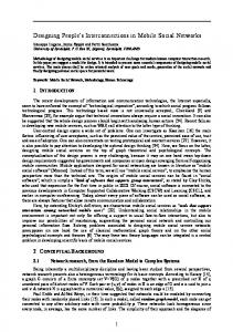
Digital signal processing (DSP) has become an important tool in consumer, communications, medical, and industrial products. A wide variety of approaches is used to implement DSP algorithms, ranging from the use of off-the-shelf microprocessors to field-programmable gate arrays (FPGA) to custom integrated circuits (IC) [37]. While programmable approaches continue to progress in performance, historical digital signal processors were unable to execute applications like rake receiver, evaluation of image sequences or radar signals [85, 106]. As programmable approaches progress, higher bit rate applications continue to gain momentum still favoring application-specific hardware. In addition, power consumption is of major concern in the design of portable devices, which favors application-specific hardware where large parallelism and low clock rate can be utilized. Unfortunately, the design of application-specific hardware is considered to be costly. This together with the ever-increasing design complexity and higher integration level have been the key drivers for system-on-chip (SoC) designs. Lower design costs require greater reuse of intellectual property, silicon implementation regularity, or other novel circuit and system architecture paradigms [57]. In order to improve the design productivity, increased reuse, freedom of choice, and pervasive automation should be utilized [33]. Parallelism of computation is often employed in application-specific hardware structures for DSP algorithms. One extreme is a fully parallel implementation where the operations in a signal flow graph are mapped directly onto functional units, which is referred to as a direct-mapped implementation. This way the maximum parallelism can be obtained allowing the minimum clock rate to be used, resulting in reduced energy per operation [17, 30]. Power efficiencies of direct-mapped hardware are up to four orders of magnitude greater than for general-purpose microprocessors, and this gap is increasing [57].

2

1. Introduction a)

x0 x8 x4 x12 x2 x10 x6 x14 x1 x9 x5 x13 x3 x11 x7 x15

interconnection

interconnection

interconnection

F2

F2

F2

F2

F2

F2

F2

F2

F2

F2

F2

F2

F2

F2

F2

F2

F2

F2

F2

F2

F2

F2

F2

F2

F2

F2

F2

F2

F2

F2

F2

F2 PE

X0 X8 X1 X9 X2 X10 X3 X11 X4 X12 X5 X13 X6 X14 X7 X15

b) 0 8 4 12 2 10 6 14 1 9 5 13 3 11 7 15

M M M M M M M M M M M M M M M M

PE PE PE PE PE PE PE PE interconnection

Fig. 1. 16-point radix-2 constant geometry FFT algorithm: a) signal flow graph, b) corresponding column structure. F2 : 2-point FFT. PE: processing element. M: multiplexer.

Direct-mapped implementations may result, however, in excessive throughput and area implying that mapping onto reduced computational resources could be economically useful. For such a design problem, linear mapping methods have been proposed [60, 85]. Most digital signal processing algorithms can be formulated as regular and iterative algorithms, which in turn are especially suitable for linear mapping to array processor structures [85]. These array processors consist of parallel processing elements computing the node functions of the signal flow graph, and an interconnection network which provides communication means between the processing elements. In the linear mapping methods, the dimensionality of signal flow graphs is reduced by using horizontal, vertical, or both projections, as described, e.g., in [85]. These mapping methods can be illustrated with fast Fourier transform (FFT) as an example. Basically, the parallel structures of FFTs can be divided into three categories: direct-mapped (fully parallel), column, and cascaded (pipeline) structures [42]. As an example, the signal flow graph of a radix-2 constant geometry FFT is depicted in Fig. 1(a) where the constant geometry refers to the constant interconnection topology between the processing columns. By applying the horizontal projection to the given signal flow graph, a column structure is obtained, as depicted in Fig. 1(b). In this structure, the computation is performed for a single column at a time and the data elements are reordered with hardwired interconnections.

3

a) x0 x8 x4 x12 x2 x10 x6 x14 x1 x9 x5 x13 x3 x11 x7 x15

interconnection 0 interconnection 1 interconnection 2

F2

F2

F2

F2

F2

F2

F2

F2

F2

F2

F2

F2

F2

F2

F2

F2

F2

F2

F2

F2

F2

F2

F2

F2

F2

F2

F2

F2

F2

F2

F2

F2

X0 X8 X1 X9 X2 X10 X3 X11 X4 X12 X5 X13 X6 X14 X7 X15

PE b) 15 7 11 3 13 5 9 1 14 6 10 2 12 4 8 0

PE

IN0

PE

IN1

PE

IN2

PE

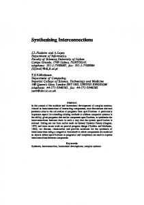
Fig. 2. 16-point radix-2 FFT algorithm: a) signal flow graph, b) corresponding cascade structure. PE: processing element. IN: interconnection network.

Cascaded structures are obtained by applying vertical projection to the signal flow graph. Consider the signal flow graph of a radix-2 FFT in Fig. 2(a), which is vertically projected resulting in a cascade structure illustrated in Fig. 2(b). In this structure, the computation is performed simultaneously on four processing columns. Such an approach implies that the interconnections require a temporal reordering of intermediate data elements, which is realized with an interconnection network having a storage capability. This is in contrast to the column structure where the interconnections are spatial and can be hardwired. Temporal interconnections are resulted also if both the horizontal and vertical projections are applied to a signal flow graph. Such a mapping produces a partial-column structure where the computation is performed for a part of the column at a time. Examples of the partial-column structures for a 16-point radix-2 constant geometry FFT are shown in Fig. 3. In all the previous parallel structures, managing the interconnections becomes crucial, which is the principal problem considered in this Thesis. The mapping onto reduced number of processing elements is made according to horizontal and vertical projections, which complicates the interconnections. Chronologically correct processing is maintained by delaying certain operands with registers or memory modules. Thus the interconnections cannot be hardwired, in general. Exceptions are direct-mapped and full column structures, where hardwired interconnections can be employed.

4

1. Introduction

1 0 9 8 5 4 13 12 3 2 11 10 7 6 15 14

M

3 1 2 0 11 9 10 8 7 5 6 4 15 13 14 12

M

7 3 5 1 6 2 4 0 15 11 13 9 14 10 12 8

M M M M M M M

M M M

M M

PE PE IN PE PE

PE IN PE

PE

IN

Fig. 3. Partial-column structures of 16-point radix-2 algorithm. PE: processing element. IN: interconnection network. M: multiplexer.

The interconnections considered in this Thesis are called stride permutations and they will be discussed in detail in the next chapter. These type of permutations have several practical applications. For example, consider a matrix transpose, which is a special case of stride permutations. Similarly, the common perfect shuffle permutation [105] is a stride permutation. The perfect shuffle has a close relation to several practical algorithms; e.g., Cooley-Tukey radix-2 FFT [24] algorithm can be scheduled into a form where the interconnections between the processing columns are perfect shuffles. In the same way, FFTs with other radices can be given in a form where interconnections are stride permutations. In this Thesis, hardware realizations of these stride permutations are referred to as stride permutation networks. Stride permutations can also be found in trellis coding and especially in Viterbi algorithm used for decoding convolutional codes. Convolutional encoders are often described with the aid of a shift register model [65]. Decoding of convolutional codes is represented with the aid of a trellis diagram [41], which is a state diagram of the convolutional encoder expressed in time. Trellis diagrams can be given in a form where operand accesses are made in stride permutation order, just like in FFTs. In addition, the processing nodes have similarities; in both algorithms, FFT and Viterbi, the number of input and output operands is K. Therefore, these types of algorithms are referred to as radix-K algorithms and their realizations as radix-K structures in the following. Typically, K is a power-of-two.

1.1. Objective and Scope of Research

5

Although the examples given in this Thesis consider FFT and Viterbi algorithms, other algorithms with the corresponding stride permutation topology exist, e.g., discrete sine, cosine, and Hartley transforms [4,108]. Currently, FFT is perhaps the most ubiquitous algorithm used to analyze and manipulate digital or discrete data [91]. It is used, e.g., in electroacoustic music and audio signal processing, medical imaging, image processing, pattern recognition, computational chemistry, error-correcting codes, spectral methods for partial differential equations, and mathematics [91]. Any time the analyzed or manipulated data set is very large and accuracy is essential, very large FFTs are required [26]. Example applications employing large FFTs are found in radio astronomy where FFTs of tens of gigapoints are used [26]. Viterbi algorithm was initially proposed for decoding of convolutional codes in [117]. Later on, it has been used as maximum-likelihood sequence estimator for detecting data signals in digital transmission [87, 99]. As a result, Viterbi algorithm has been adopted in consumer products like magnetic storage devices [86], modems [35, 53, 54], DVB [36], DAB [34], DVD players [47], and mobile phones [111]. It has also been used in other areas such as character recognition, voice recognition, and DNA analysis, to name few examples. The algorithm is so fundamental that one would expect ever-widening application [48].

1.1 Objective and Scope of Research The objective of this Thesis is to develop systematic design methods for stride permutation interconnections. Such design methods alleviate substantially automatic design generation. Therefore, the structures realizing the stride permutation interconnections are described with the aid of design parameters such as the size of permutation, stride, and the number of input/output ports. All the parameters are assumed to be powers-of-two. As the first objective, a systematic design method for stride permutation networks consisting of delay registers and multiplexers is to be developed. These networks are referred to as register-based stride permutation networks in the following. The problem to be solved is to derive the networks with the aid of decompositions of stride permutation matrices. The networks should have minimum register and multiplexer complexities.

6

1. Introduction

The second objective is to develop a systematic design method for stride permutation networks based on a parallel memory system. Such networks are called memorybased stride permutation networks in the following. The problem in this approach is to find an access scheme that supports all power-of-two stride permutations. The amount of memory and the complexities of control and interconnections should be kept in minimum.

1.2 Main Contributions In this Thesis, systematic design methods for stride permutations are developed. To summarize, the main contributions are the following: • Survey of previous work in hardware realizations of stride permutations. • Systematic method for deriving hardware structures based on decompositions of stride permutation matrices. – Decompositions of stride permutation matrices, which can be mapped directly onto hardware. – Register-based stride permutation networks, which have the lowest register and multiplexer complexities presented so far. • Two systematic methods for designing memory-based stride permutation networks: low control complexity scheme and low interconnection complexity scheme. – Low control complexity scheme, which supports stride and bit reversal permutations, uses minimum amount of memory, and results in simple row address generation. – Low interconnection complexity scheme, which uses minimum amount of memory and results in reduced interconnection complexity by rescheduling the operations. • Derivation of lower bound for register complexity in stride permutations.

1.3. Thesis Outline

7

1.2.1 Author’s Contribution The author derived the decompositions of stride permutation matrices and developed and analyzed the register-based stride permutation networks. In addition, derivation of the lower bound for register complexity as well as the comparison against other reported structures were carried out by the author. The studies on register-based stride permutation networks have been reported earlier in [109], [P1, P2, P3]. In general, these earlier networks do not result in the minimum register complexity thus the work has been continued in [P6] and [P7] where the design method resulting in minimum register complexity is introduced for the first time. The author was responsible for verifying the low control complexity scheme, which has been initially published in [P4]. In addition, the low interconnection complexity scheme, which has been published in [P5] and [P8], was developed and verified by the author. The author conducted the comparison against the earlier published schemes. The work reported in this Thesis has been published earlier in eight publications [P1P8]. Therefore, some chapters contain verbatim extracts from the publications. These extracts are under copyright of respective copyright holders. None of the publications has been used in another person’s academic thesis.

1.3 Thesis Outline To start with, permutations and their presentations are reviewed in Chapter 2. A class of permutations called bit-permute/complement permutations as well as its subclass, stride permutations, are defined. In Chapter 3, a review of previous work on the realizations of stride permutations is made. The review is divided into three parts: switching, register-, and memory-based networks. Some traditional interconnection means are reviewed followed by more application-specific structures. In the context of memory-based networks, parallel memory systems are defined, some principal access schemes are reviewed, and a stride permutation access scheme is defined. In addition, some parallel memory structures used in FFT and Viterbi computations are reviewed. Chapter 3 contains some material already published in [P4, P8]. In Chapter 4, a new systematic design method for register-based stride permutation networks is proposed. First, stride permutation matrices are decomposed into smaller

8

1. Introduction

block-diagonal matrices starting from a square matrix transpose. The square matrix transpose is the basis for other stride permutations, which are decomposed subsequently. Some examples of decompositions are provided with fixed design parameters. Then, the mapping of the decompositions onto hardware structures is discussed. A lower bound of register complexity is derived and register and multiplexer complexities of the proposed networks are given. The chapter is concluded with a comparison against the other reported register-based networks. Some parts of this Chapter have been published earlier in [P1–P3, P6, P7]. Memory-based stride permutation networks for stride permutations are developed in Chapter 5. First, a low control complexity scheme is defined by specifying the row and module addresses and control generation. Then, a low interconnection complexity scheme is developed where the rescheduling of operations is suggested followed by the definition of a row address generator. An example design is provided with fixed design parameters and complexity figures are given. At the end, an overview and comparison of different parallel memory structures for FFT and Viterbi algorithms are given. Some material in Chapter 5 has been reported in [P4, P5, P8]. Chapter 6 concludes the Thesis.

2. PERMUTATIONS

In this chapter a class of permutations referred to as stride permutations is reviewed. The stride permutations are a subclass of bit-permute/complement (BPC) permutations, which are named after the index mapping method, i.e., the permuted data sequence is obtained by permuting and complementing the index bits of the initial data sequence. In such a way, a rich number of permutations can be defined including, e.g., matrix transpose, bit reversal, vector reversal, shuffle permutations [25, 75]. The chapter is organized as follows. First, different representations of permutations are reviewed. Then, BPC permutations are defined according to [25] followed by the definition of a subclass of BPC permutations. This subclass considers stride permutations, which are discussed throughout the thesis. At the end of this chapter, some preliminaries for mathematical representation of stride permutations are given.

2.1 Definitions A permutation, in general, is defined as follows [72]: Definition 1 (Permutation): 1. The arrangement of any determinate number of things, as units, objects, letters, etc., in all possible orders, one after the other; called also alternation. 2. Any one of such possible arrangements. [72] Permutations can be represented in several different ways. One often used method is based on permutation matrices. Definition 2 (Permutation Matrix): A permutation matrix PN is an N × N matrix with all elements either 0 or 1, with exactly one 1 at each row and column. [74]

10

2. Permutations

As an example, a matrix P, ⎛

⎞ 0 1 0 ⎜ ⎟ P = ⎝ 0 0 1 ⎠, 1 0 0 is a permutation matrix. Let A be a matrix ⎞ ⎛ 1 2 3 ⎟ ⎜ A = ⎝ 4 5 6 ⎠. 7 8 9 Then PA is a row-permuted version of A, and AP is a column-permuted version of A: ⎞ ⎞ ⎛ ⎛ 3 1 2 4 5 6 ⎟ ⎟ ⎜ ⎜ AP = ⎝ 6 4 5 ⎠ . PA = ⎝ 7 8 9 ⎠ ; 9 7 8 1 2 3 Permutation matrices are orthogonal: if P is a permutation matrix, then P−1 =PT . The product of permutation matrices is another permutation matrix. [74] The second method for the representation of permutations is to use an index function f (i). With such an index function, the data sequence X, X = (x0 , x1 , . . . , xN−1 ), is reordered as Y , Y = (y0 , y1 , . . . , yN−1 ) where yi is given as yi = x f (i) ,

or

y f −1 (i) = xi .

(1) (2)

In this thesis, the index functions will be used as given in (1), where the data sequence X is reordered as Y , Y = (x f (0) , x f (1) , . . . , x f (N−1) ). Third method of using the index functions is based on their definition of bit positions of the index in binary form, as done in bit-permute/complement permutations.

2.2 Bit-Permute/Complement Permutations Initially, the BPC permutations were defined by Nassimi and Sahni in [75] where they suggested an algorithm to route data in a mesh-connected parallel computer. The suggested algorithm supports any permutation, which can be represented as permuting and complementing of the bits of a processor address. The bit permutation

2.2. Bit-Permute/Complement Permutations

11

is made according to bit index function, π(i), which is fixed, i.e., it is the same for each address. The bit permutation may also be accompanied by complementing the fixed set of address bits. Thus the name bit-permute/complement permutation. Since the processor address is obtained by permuting the address bits, it is required that the number of processors is a power-of-two [92]. Consider that permutation of elements is a one-to-one mapping of input addresses from the set {0, 1, . . . , N − 1} onto itself, i.e., the source address of element a = (an−1 , an−2 , . . . , a0 ) is mapped onto target address b = (bn−1 , bn−2 , . . . , b0 ), where n = log2 N. The leftmost bit represents the most significant bit. In BPC permutations, the target address b is formed from its source address a by applying a fixed bit permutation π(i) to the address bits and then complementing a fixed subset of bits of the result. The complementing is equivalent to exclusive-oring (XOR) by an n-bit complement vector c, c = (cn−1 , cn−2 , . . . , c0 ). A source address a maps to a target address b by the equation b j = aπ( j) ⊕ c j ,

j = 0, 1, . . . , n − 1,

(3)

where ⊕ represents a bitwise XOR operation. Besides [75], BPC permutations have been discussed, e.g., in [25, 32, 77, 92]. According to [25, 75], many familiar permutations fall into a class of BPC permutations. For example, a perfect shuffle permutation [105] is a BPC permutation defined as π( j) = j + 1 mod n , j = 0, 1, . . . , n − 1, (4) cj = 0 where mod represents a modulo operation. An example of perfect shuffle permutation applied to a 16-element data sequence is shown in Fig. 4(a). Another example is a bit shuffle permutation where the number of bits n is even. The bit shuffle permutation is expressed as π( j) = 2 j mod n , j = 0, 1, . . . , n − 1. (5) cj = 0 A bit shuffle permutation is illustrated with a 16-element data sequence in Fig. 4(b). Similarly, a bit reversal permutation belongs to BPC permutations. In the bit reversal permutation, the bits of the source address of each element (an−1 ,an−2 ,. . . ,a0 ) are

12

2. Permutations a) 0

0

b) 0

0

c) 0

0

d) 0

15 e) 0

1

8

1

1

1

8

1

0

14

1

4

2

1

2

4

2

4

3

9

3

5

3

12

2

13

2

8

3

12

3

12

4

2

4

2

4

5

10

5

3

5

2

4

11

4

1

10

5

10

5

5

6

3

6

6

6

6

6

9

6

9

7

11

7

7

8

4

8

8

7

14

7

8

7

13

8

1

8

7

8

2

9

12

9

9

9

9

9

6

9

6

10

5

10

12

10

5

10

5

10

10

11

13

11

13

11

13

11

4

11

14

12

6

12

10

12

3

12

3

12

3

13

14

13

11

13

11

13

2

13

7

14

7

14

14

14

7

14

1

14

11

15

15

15

15

15

15

15

0

15

15

Fig. 4. BPC permutations on 16-element data arrays: a) perfect shuffle, b) bit shuffle, c) bit reversal, d) vector reversal, and e) 4 × 4 matrix transpose.

reversed to form the element’s target address (a0 , . . . , an−2 , an−1 ), which is expressed as π( j) = n − 1 − j , j = 0, 1, . . . , n − 1. (6) cj = 0 An example of bit reversal permutation is given in Fig. 4(c). Furthermore, vector reversal permutations are BPC permutations. In vector reversal permutations, the source address i is mapped to the target address (N − 1) − i, i = 0, 1, . . . , N − 1, which is performed by complementing all the bits of the source address, i.e., π( j) = j , j = 0, 1, . . . , n − 1. cj = 1

(7)

An example of the vector reversal permutation is shown in Fig. 4(d). A matrix transpose can also be thought as a BPC permutation. Consider a transpose of an S × V matrix. The operation can be described with an SV -element vector as follows; first the elements of the matrix are read into a vector in column-wise. Then, the elements are reordered according to a permutation

π( j) = j + v mod s + v , j = 0, 1, . . . , s + v − 1. cj = 0

(8)

2.3. Stride Permutations

13

where s = log2 S, v = log2 V . After the permutation, the elements are written back into a S ×V matrix in column-wise. In Fig. 4(e), a 4 × 4 matrix transpose is depicted.

2.3 Stride Permutations The described matrix transpose is also known as a stride permutation; stride-by-S permutation of an N-element vector can be performed by dividing the vector into Selement subvectors, organizing them into S × (N/S) matrix form, transposing the obtained matrix, and rearranging the result back to the vector presentation [44]. This interpretation implies that the stride S has to be a factor of vector length, i.e., N rem S = 0 where rem denotes remainder after division. In the stride permutations, the address bits are shifted cyclically without complementation. Thus, they are also called shuffle permutations, as done in [29]. A stride-by-S permutation of an N-element sequence can be represented as

π( j) = j + s mod n , j = 0, 1, . . . , n − 1. cj = 0

(9)

Since the binary representation of permutations is used, only power-of-two strides are possible. In the following, the discussion is limited to power-of-two stride permutations. Another representation for stride permutations is given with an index function as follows; Definition 3 (Stride Permutation): Let us assume a vector X = (x0 , x1 , . . . , xN−1 ). Stride-by-S permutation reorders X as Y = (x fN,S (0) , x fN,S (1) , . . . , x fN,S (N−1) )T where the index function fN,S (i) is given as fN,S (i) = (iS mod N) + iS/N | N rem S = 0, i = 0, 1, . . . , N − 1

(10)

where · is the floor function. For the matrix representation of stride permutations, the stride-by-S permutation ma-

14

2. Permutations

trix of order N is defined as

[PN,S ]mn =

1, iff n = (mS mod N) + mS/N , 0, otherwise

m, n = 0, 1, . . . , N − 1.

(11)

For example, the permutation matrix P8,2 associated to stride-by-2 permutation of an 8-element vector is the following (blank entries represent zeros): ⎛ ⎞ 1 ⎜ ⎟ 1 ⎜ ⎟ ⎜ ⎟ ⎜ ⎟ 1 ⎜ ⎟ ⎜ ⎟ 1 ⎟. P8,2 = ⎜ ⎜ ⎟ 1 ⎜ ⎟ ⎜ ⎟ 1 ⎜ ⎟ ⎜ ⎟ 1 ⎝ ⎠ 1 By multiplying the source vector with a permutation matrix, the stride permutation is performed, i.e., Y = PN,S X where X and Y are the source and reordered vectors, respectively, and PN,S is the stride-by-S permutation matrix of order N. As an example, P8,2 (0, 1, 2, 3, 4, 5, 6, 7)T = (0, 2, 4, 6, 1, 3, 5, 7)T

(12)

where T represents a transpose. In this Thesis, the discussion is limited to practical cases where the strides and array lengths are powers-of-two, N = 2n , S = 2s . Some properties of stride permutations in such cases are given in the following.

2.4 Preliminaries for Matrix Representation of Stride Permutations For ordinary products of matrices, left evaluation is used, i.e., n

∏ Ai = (((A0 · A1 ) · A2 ) · . . . · An ).

(13)

i=0

The formulation used here is based on tensor products: tensor product (or Kronecker product) is denoted by ⊗. The proofs for the following theorems can be found, e.g., in [29] and [44].

2.4. Preliminaries for Matrix Representation of Stride Permutations

15

Theorem 1 (Factorization of stride permutations): Pa,bc = Pa,b Pa,c

(14)

Pabc,c = (Pac,c ⊗ Ib ) (Ia ⊗ Pbc,c )

(15)

where IK denotes the identity matrix of order K. Corollary 1 (Periodicity): Stride permutations are periodic with the following properties. 1) Period of P2n ,2s is lcm(n, s)/s where lcm(a, b) denotes the least common multiple of n and s. In other words, lcm(n,s)/s

I2n =

∏

P2n ,2s .

(16)

1

2) Consecutive stride permutations always result in a stride permutation: P2n ,2a P2n ,2b = P2n ,2(a+b) mod n .

(17)

Proof. Property 2) If a+b > n, the left side of (17) can be written as P2n ,2kn+(a+b) mod n = P2n ,2kn P2n ,2(a+b) mod n where k > 1 is an integer. By substituting 2n for S in (10), we find that P2n ,2n = P2n ,1 = I2n . Therefore, P2n ,2kn = I2n and the result follows. Property 1) Let us assume that period of P2n ,2s is k, thus ks mod n = 0, i.e., ks is a multiple of n. This implies that k is a multiple of n/s, i.e., k = mn/s. k has to be integer, thus s has to be a factor of mn. The smallest number fulfilling the requirement is lcm(n, s) and, therefore, k = lcm(n, s)/s. Theorem 2 (Relationship between tensor product and stride permutation): If Aa and Bb are matrices of order a and b, respectively, then, Aa ⊗ Bb = Pab,a (Bb ⊗ Aa ) Pab,b .

(18)

Theorem 3. The transpose of a matrix product is the product of the transposes in reverse order: (ABC)T = CT BT AT .

(19)

16

2. Permutations

Finally, a special permutation matrix JK of order K is defined as

or alternatively as

JK = I2 ⊗ PK/2,K/4 PK,2

(20)

JK = PK,K/2 I2 ⊗ PK/2,2 .

(21)

The permutation JK exchanges the odd elements in the first half of a vector with the even elements of the last half of the vector. Based on the properties of tensor product and stride permutations, the following property holds: JN ⊗ IM = IN/2 ⊗ P2M,2 JNM IN/2 ⊗ P2M,M ,

N = 2n > M = 2m .

(22)

3. PREVIOUS WORK

Managing data permutations in the parallel hardware implementations of digital signal processing algorithms is crucial. Especially in partial column and cascaded structures, the complexity of permutations is increased since data elements must be delayed in order to meet chronologically correct processing. In this chapter, three principal approaches for the hardware realization of stride permutations are reviewed: switching, register-, and memory-based networks. The focus in the review is on the scalability and stride permutation support of the networks. Similarly, the realization complexity in terms of registers and multiplexers and memory usage is studied. In addition, the complexity of design process is considered. The first section begins with common switching networks, which have been rigorously studied in supercomputing area. It is remarked that such networks cannot be utilized for stride permutations performed over less number of ports than the sequence size due to the absence of storage registers. For managing the storage problem, the register-based networks are studied in the second section. Such networks are divided into one- and two-dimensional networks and further into application specific networks. In order to reduce the complexity of such networks, a register minimization methodology is reviewed. The third section is limited to memory-based structures. At first, two principal types of memory systems are reviewed: time-multiplexed (interleaved) and spacemultiplexed (parallel) memory systems. Then, some principle access schemes are discussed including low order interleaving, row rotation, and linear transformation. After that, a specific access pattern called stride access, which is one of the common access patterns discussed in several research papers, is reviewed. From the stride access, the discussion is continued with a stride permutation access, which is rarely considered by the earlier research of parallel memory systems. Differences between stride access and stride permutation access are emphasized. At the end of this chap-

18

3. Previous Work

ter, a review of parallel Viterbi and FFT structures with parallel memory systems is made. The chapter is concluded with a brief summary.

3.1 Switching Networks Over the years, a lot of research effort has been placed on interconnection networks used in multiprocessor architectures for connecting processors and memories together. The problem of data interconnections is found also in other fields including telecommunications where routers are used for switching data packets [22], and driven by the growing integration level in silicon, also in system-on-chip (SoC) designs where networks-on-chip (NoC) are used for connecting components like processors, controllers, and memory arrays [9]. In general, there is a wide variety of applications where the realizations of data interconnections are needed. Interconnection networks can be classified, e.g., based on timing philosophy, switching methodology, or control strategy [10]. On the other hand, network topologies can be used in the classification; there are, e.g., single- and multistage networks which refer to topologies where one or several stages of switching elements are used, respectively. Furthermore, many permutations share commonalities thus the networks can also be classified based on the class of permutations they support. As an example, a class of networks for bit-permute/complement permutations is proposed in [2]. Because of such a wide variety, determining the best network for a certain application is a difficult task and requires a careful selection of the metrics for the comparison [66]. The discussion in this Thesis is limited to networks which support stride permutations. A network illustrated in Fig. 5 is called a crossbar network which is an example of switching networks performing arbitrary permutations between the input and outputs. In the figure, Q processing elements communicate through Q memories and the crossbar network provides conflict-free communication paths such that a processing element can access any memory module if there is no other element reading or writing in the same module. The paths between the inputs and outputs in the network are realized with Q2 crosspoint switches, which makes the network infeasible for large systems [98].

19

3.1. Switching Networks

B0

B1

BQ-1

PE0 PE1 crosspoint switch PEQ-1

Fig. 5. Crossbar network connecting Q processing elements to Q memory modules [98]. PE: processing element. B: memory module.

In general, the networks with the capability of passing all the N! permutations on N elements in one pass through the network are known as rearrangeable networks [8]. These rearrangeable networks are also called as permutation networks [15]. Stone presented in [105] shuffle/exchange (SE) networks based on perfect shuffle permutations. One stage in a Q-port SE network consists of a hardwired perfect shuffle permutation of size Q followed by Q/2 switches of type 2 × 2. Examples of such networks are depicted in Fig. 6 where a single-stage SE network and a log2 Q -stage SE network called Omega network [63] are shown. The capability of performing arbitrary permutations, i.e., rearrangeability, with the SE networks has been studied, e.g., in [67, 116]. In such papers, one of the main problems to be solved considers finding the minimum number of stages needed for performing arbitrary permutations. In case of a single-stage SE network, the minimum number of passes is studied. Although a theoretical lower bound of 2 log2 Q − 1 stages of 2 × 2 switches is known [118], the sufficiency of such bound for SE networks has neither been proved or disproved [116]. A well-known rearrangeable network is the Benes network [8], which is built in a recursive manner by using 2 × 2 switches. A Q-port Benes network consists of 2 log2 Q − 1 stages of Q/2 switches in parallel. An example of 8-port Benes network built up from 4-port Benes networks is shown in Fig. 7. For the Benes networks, studies have been conducted for developing schemes for setting the switches concurrently with data propagation, e.g., in [76, 90].

20

3. Previous Work a)

b)

c)

S

S

S

S

S

S

S

S

S

S

S

S

S

S

S

S

0

1

Fig. 6. 8-port shuffle/exchange networks: a) single-stage SE network, b) Omega network, and c) connection patterns. S: switch.

S

S

S

S

S

S

S

S

S

S

S

S

S

S

S

S

S

S

S

S

Fig. 7. 8-port Benes network where 4-port Benes network is shown with dashed lines. S: switch.

The drawback of switching networks, of which the preceding networks are examples, is that they cannot be used for stride permutations performed in parts with less number of ports than the size of the permutation. As an example, consider the perfect shuffle permutation of 8 data elements. With a single-stage SE network such permutation can be performed with straight connected switches, as depicted in Fig. 8(a). On the other hand, consider the same permutation divided into four parts such that two data elements enter the network at a time, as shown in Fig. 8(b). The network in this case is a 2-port SE network, which actually reduces to a 2-port switch. In such a case, the elements 0 and 4 should be the first two data elements at the output. However, the elements 0 and 1 enter the network at a time, thus the element 0 should be delayed two cycles until the element 4 is available at the input. With the switching networks, such an arrangement is not possible. Therefore, the networks where registers are used for delaying the data elements are discussed in the following. Such networks are referred to as register-based networks.

21

3.2. Register-Based Networks a)

b)

0

0

4

1

4

2

1

2

3

5

3

6

4

2

0

3

2

1

0

5

4

2

4

7

5

3

1

7

6

5

4

2

5

6

5

6

6

3

6

3

7

7

7

7

0

0

1

t=3

1

t=2 t=1 t=0

Fig. 8. Perfect shuffle permutation with: a) 8-port single-stage SE network, b) 2-port SE network resulting in conflicts. t: time instant.

3.2 Register-Based Networks Because the switching networks cannot be used for stride permutations performed over less number of ports than the sequence size, register-based networks are reviewed in this section. The variation among register-based networks is considerable thus the review is limited to networks which support stride permutations. The discussion is divided into one- and two-dimensional networks based on the network topologies; the one-dimensional networks operate over sequential data streams while the two-dimensional networks are applied to parallel data streams. In the initial context, some of the reviewed networks are referred to as data format converters. For simplicity, they are called as permutation networks in this Thesis.

3.2.1 One-Dimensional Networks In [96], Shung et al. proposed a one-dimensional permutation network based on shift exchange units (SEU), which supports arbitrary data permutations over sequential data streams. The structure of a SEU of size D, SEUD , is depicted in Fig. 9(a). It consists of a delay line of D registers and two multiplexers, which either inputs the data element into the delay line or bypasses it. The bypass results in the exchange of data elements which are D elements apart in the data stream. A one-dimensional permutation network consisting of log2 N − 1 cascaded SEUs is shown in Fig. 9(b). One method of reducing the network complexity is proposed by Parhi in [79, 82]. This systematic methodology minimizes the number of registers based on the life time analysis of data elements. In general, the data elements have different life times

22

3. Previous Work a)

ci

SEUD

M

b)

c1

c3

c5

SEU1

SEU2

SEU4

D

D D delays

c2(log N)-1 2 SEUN/2

M

c6

c4

c2

SEU4

SEU2

SEU1

Fig. 9. One-dimensional permutation network [96]: a) shift exchange unit (SEU), b) permutation network of log2 N − 1 stages of SEUs. N: number of data elements. D: number of delay registers. c: control signal. M: 2-to-1 multiplexer. D: delay register.

making the reuse of registers possible. In such a case, a new data element can be assigned to a register if the former data element is read out. Although the method was initially proposed for one-dimensional networks, it can be applied to two-dimensional networks as well. In Table 1, an example case of the life time analysis of a 4 × 4 matrix transpose is shown. The network operates in sequential manner, and the clock cycles for the data element input and output are denoted as tinput and tout put , respectively. The difference between the output and input cycles is denoted as tdi f f , i.e., tdi f f = tout put −tinput . The absolute value of the most negative tdi f f determines the minimum number of registers, and it is added to each tdi f f for obtaining the life time l(i) of a data element i. The life period denotes the cycles when the data element must be stored in the network. In case of the 4 × 4 matrix transpose over sequential data stream, overall nine registers are required. Based on the life time analysis, Parhi proposed several types of register-based permutation networks in [80]. The networks are divided into various classes according to the number and the size of the input and output words. However, the operation of all the networks is sequential although they may have multiple input and output ports. A forward-circulate register allocation scheme begins with first calculating the minimum number of registers and connecting them into a chain. The data elements are read in one at a time and forwarded to the next register if the register is available. Otherwise, the data element is circulated, i.e., read again by its current register. In

23

3.2. Register-Based Networks

Table 1. Life time analysis of data elements for one-dimensional 4 × 4 matrix transpose network [82]. tinput : clock cycle of data element input. tout put : clock cycle of data element output. tdi f f =tout put − tinput . l(i): life time of data element. data element

tinput

tout put

tdi f f

l(i)

life period

0 1 2 3 4 5 6 7 8 9 10 11 12 13 14 15

0 1 2 3 4 5 6 7 8 9 10 11 12 13 14 15

0 4 8 12 1 5 9 13 2 6 10 14 3 7 11 15

0 3 6 9 -3 0 3 6 -6 -3 0 3 -9 -6 -3 0

9 12 15 18 6 9 12 15 3 6 9 12 0 3 6 9

0→9 1 → 13 2 → 17 3 → 21 4 → 10 5 → 14 6 → 18 7 → 22 8 → 11 9 → 15 10 → 19 11 → 23 12 → 12 13 → 16 14 → 20 15 → 24

certain cases, the forward-circulate scheme results in deadlocks, which implies that the data element cannot be forwarded or circulated [80]. Compared to the previous scheme, a forward-backward allocation scheme results in a register chain with simpler control. The most important advantage, however, is that the forward-backward scheme never results in deadlocks. Thus, the scheme can be used for arbitrary permutations. In the scheme, all the data elements with life times less or equal to the number of registers are allocated in a forward manner until they are read out or they reach the last register. Data elements that cannot be forwarded are backward allocated to some available registers so that required feedback connections are minimized. A 4 × 4 matrix transpose network based on the forward-circulate register allocation scheme is shown in Fig. 10(a). In such a case, each register has a feedback connection from its output and a multiplexer in its input for circulating the data elements. In Fig. 10(b), a 4 × 4 matrix transpose network based on the forward-backward allocation scheme is illustrated. It contains less multiplexers and the same amount of registers as the network based on the forward-circulate scheme. Later on in [81],

24

3. Previous Work

a) M M

D0

M

D1

M

D2

M

D3

M

D4

M

D5

M

D6

M

D7

M

D8

b) M M

D0

D1

D2

M

D3

D4

D5

M

D6

D7

D8

Fig. 10. 4×4 matrix transpose networks based on a) forward-circulate, b) forward-backward register allocations [80]. D: register. M: multiplexer.

Parhi applied the forward-backward register allocation scheme to data permutations in video applications. Applying one-dimensional networks to permutations in parallel data streams requires that either the frequency of the network is increased or that multiple one-dimensional networks are used in parallel. In the latter case, additional interconnection lines between the networks may be required, which increases the network complexity. For managing the interconnection, register, and multiplexer complexities, the networks, which are initially designed to operate over parallel data streams, are proposed. Such networks are called two-dimensional networks based on their topology, and they are discussed in the following.

3.2.2 Two-Dimensional Networks The general approach in two-dimensional permutation networks is that the data elements are reordered with switching elements on parallel delay lines. In these networks, an exchange of data elements between the delay lines is often needed, which in turn results in additional multiplexers and connection wirings. Although the minimization of register complexity is still one of the design objectives, there are several schemes where also the reduction of multiplexer and interconnection complexities and power consumption are devoted to. Next, the discussion is continued with twodimensional permutation networks supporting arbitrary permutations.

25

3.2. Register-Based Networks a)

time Input

t=1

t=2

t=3

t=4

t=5

t=6

t=7

0 1 2 3 4 5 6 7 8 9 10 11 12 13 14 15

D0 D1 D2 D3

0 1 2 3 4 5 6 7 8 9 10 11 3 13 14 15 0 1 2 3 4 5 6 7 2 9 10 11 3 7 14 15

D4 D5 D6 D7 D8 D9 D10D11

0 1 2 3 1 5 6 7 2 6 10 11 3 7 11 15

Output

0 4 8 12 1 5 9 13 2 6 10 14 3 7 11 15 b) M D0

D1

D2

D3

M

M

D4

D5

D6

D7

M

M

M

D8

D9

D10

D11

M

M

M

Fig. 11. Two-dimensional 4 × 4 matrix transpose network [6]: a) register allocation table, b) resulting network. M: multiplexer. D: register.

Bae and Prasanna presented in [6, 7] a design methodology for two-dimensional permutation networks resulting in the minimum number of registers. In Fig. 11, the methodology is illustrated with a 4 × 4 matrix transpose where four data elements are read in and written out in parallel. First, the minimum number of registers is determined. Then, the data is allocated to the registers such that at each clock cycle the parallel shifting is carried out. When all the data elements are available for the output, they are written out immediately. A backward allocation of the data elements is illustrated with the arrows in the register allocation table in Fig. 11(a). Such allocation is needed when the parallel shifting moves the data elements forward in the delay lines and there is not enough registers before the output. Moving the data elements inside the network and passing the data elements to output imply a need for multiplexers. The circles in Fig. 11(a) denote that the data element is passed to output. The resulting structure of 4 × 4 transposer is illustrated in Fig. 11(b). It is worth noting that the methodology has limitations among the stride permutations: it does not support cases where the number of ports is less than the stride.

26

3. Previous Work

In a low-power register allocation scheme suggested by Srivatsan et al. in [103, 104], the main objective is the reduction of power consumption, not the minimization of area although the minimum number of registers is obtained. In addition, the proposed scheme supports arbitrary permutations. Compared to the previous schemes, the data elements stay in a single register as long as possible instead of moving forward at each cycle. The resulting networks have gated clocks, more multiplexers, and larger area compared to the Parhi’s one-dimensional networks [104]. As an example, due to the reduced data element transitions, the power consumption of a one-dimensional 4 × 4 matrix transposer is shown to be 42% lower and area two times larger compared to Parhi’s network in Fig. 10(b) [104]. Majumdar and Parhi proposed a register allocation scheme for arbitrary permutations in [71]. The resulting network has a two-dimensional structure where an attempt is placed on the minimization of interconnection wirings. The proposed approach begins with the life time analysis for determining the minimum number of registers. Thereafter, the network is constructed where the number of parallel delay lines is equal to the number of input ports. Available interconnection wirings are reused, if possible, and clock gating is exploited for power savings. In general, the described design methodologies for two-dimensional networks involve heuristics, which makes an automated design generation difficult [6]. Such design methodology can be given as an integer linear programming (ILP) model, which is resolved with an ILP solver in order to determine the network structure, i.e., the register allocation, interconnections, and the placement of multiplexers, as done in [103, 104]. This is computationally a very intensive task especially when large number of registers is used. It may take considerable amount of time to find a solution which obviously is a drawback on the automated design generation. In addition, control generation may be complex because of the arbitrary structure of the networks.

3.2.3 Application Specific Networks The previous networks support arbitrary permutations thus they are not designed for a particular application. Instead, the aim in designing of such networks has been to support as many permutations as possible. In the following, the discussion is continued with register-based networks, which are designed for stride permutations. Often, such networks can be found, e.g., in FFT, DCT, or Viterbi algorithm implementations.

27


2

6

0

1

7

0

8

2 10 4 12 6 14

8

9 10 11 12 13 14 15

1

9

3 11 5 13

3

4

5

7 15

16 17 18 19 20 21 22 23

16 24 18 26 20 28 22 30

24 25 26 27 28 29 30 31

17 25 19 27 21 29 23 31

32 33 34 35 36 37 38 39

32 40 34 42 36 44 38 46

40 41 42 43 44 45 46 47

33 41 35 43 37 45 39 47

48 49 50 51 52 53 54 55

48 56 50 58 52 60 54 62

56 57 58 59 60 61 62 63

49 57 51 59 53 61 55 63

0

8 16 24 4 12 20 28

0

8 16 24 32 40 48 56

1

9 17 25 5 13 21 29

1

9 17 25 33 41 49 57

2 10 18 26 6 14 22 30

2 10 18 26 34 42 50 58

3 11 19 27

7 15 23 31

3 11 19 27 35 43 51 59

32 40 48 56 36 44 52 60

4 12 20 28 36 44 52 60

33 41 49 57 37 45 53 61

5 13 21 29 37 45 53 61

34 42 50 58 38 46 54 62

6 14 22 30 38 46 54 62

35 43 51 59 39 47 55 63

7 15 23 31 39 47 55 63

Fig. 12. Example of iterative method for 8 × 8 matrix transpose according to [16].

In [16], Carlach et al. proposed an iterative method for the transpose of X × X square matrices, X = 2x . The method can be described with successive submatrix transposes as depicted in Fig. 12. In the first step, the matrix is divided into 2×2 submatrices and each submatrix is transposed. In the second step, the resulting matrix is divided into 4×4 submatrices and each submatrix is interpreted to consist of four 2×2 blocks and such a matrix is transposed in blockwise. By continuing such steps x times the entire matrix is transposed. The realization of the described method is shown in Fig. 13(a) consisting of delay-switch-delay (DSD) units depicted in Fig. 13(b). The DSDD unit has two data paths both of them having D registers for delaying the data elements and a 2 × 2 switch for swapping the elements between the paths. The described network has the minimum number of registers and it can be applied for square matrix transposes performed over X parallel data streams where X is a power-of-two. A commutator is a generic permutation unit in structures where one processing element is used, e.g., in [73], or in cascaded (pipelined) structures [20,56,107] where several processing elements operate in parallel and intermediate data permutations are performed with aid of commutators, initially proposed by Rabiner and Gold in [88]. An example of 4-port commutator, which can be used for data permutations, e.g., in

28

3. Previous Work a)

b) DSD 1

DSD 2

DSD 4

DSD 1

DSD 2

DSD 4

DSD 2

DSD 4

DSD 1

DSD 2

DSD 4

D delays

D delays D

clk DSD 1

c

DSDD ...

D

S

0

...

D

D

1

Fig. 13. Permutation network for 8 × 8 matrix transpose: a) network structure, b) delayswitch-delay (DSD) unit and switch connection patterns, S: switch. D: register. c: control. clk: clock. a)

b) D D D D D D

D D

S

D

D D D

Fig. 14. Commutator for radix-4 FFT: a) structure, b) connection patterns. D: register. S: switch.

radix-4 FFTs, is shown in Fig. 14(a) and the corresponding connection patterns in Fig. 14(b). An example of cascade structures employing such commutator is illustrated in Fig. 15 with a 64-point radix-4 FFT structure proposed by Jung et. al in [56]. In [21], a comparison of different commutators for radix-4 FFTs is given. The drawback of the commutators is that the switch becomes a complex unit when the number of ports is increased. Kovac and Ranganathan suggested in [59] a matrix transpose network where the transpose is carried out according to its direct interpretation, i.e., rows in and columns out. The data elements are read in and written out one element at a time. After all the data elements are read in the network, they are copied in parallel to the cor-

D-12 PE

D-4 D-8 D-12

S

D-4 D-8

PE PE

D-3 D-1 D-2

S

D-2 D-1

PE PE PE

D-3

Fig. 15. Cascaded 64-point FFT structure [56]. PE: processing element. D-X: chain of X registers. S: switch.

29


Input

D

D D

D

D D

D D

D

D D

D D

D D

D

D

D

D D

D

D D

D D

D

D

D

D

D

D D

D D

D D

D

D

D D

D D

D

D

D

D D

D

D

D

D

D

D

D

D

D

D

D

D

D

D

D

D

D

D

D

D

D

D

D

D D

D

D

D

D

D

D

D

D

D

D

D

D D

D

D

D

D

D

D D

D

D

D

D

D

D

D

D D

D

D

D

D

D

D

D

D D

D

D

D

D

D

D

D

D D

D

D

D

D D

D D

D

D Output

Fig. 16. One-dimensional network for 8 × 8 matrix transpose [59]. D: register.

responding adjacent registers, which are connected in column wise. A drawback of such approach is that the latency is increased since all the data elements must be in the network before the first column can be written out. Another drawback is that the approach does not result in the minimum register complexity but requires 2N 2 registers for an N × N matrix transpose. In Fig. 16, such a network is illustrated for 8 × 8 matrix transposes. In [2], Alnuweiri and Sait proposed two-dimensional networks for BPC permutations. In Fig. 17(a), the principal block diagram of such a network is depicted. The network consists of five permutation stages; three of them are hardwired permutations and two consist of parallel N/Q × N/Q matrix transposes where N is the number of data elements in the sequence and Q is the number of ports in the network. For the matrix transposes, they applied a network which performs the transposes according to its direct interpretation; a column is written in at a time, and after all the columns are available, the rows are read out one at a time. An example of the matrix transpose network is depicted in Fig. 17(b), which is capable of performing 4 × 4 matrix transposes. A drawback of these networks is that they do not result in the minimum number of registers. In [13], Bòo et al. proposed a structure for stride permutations based on parallel tapped first-in, first-out (FIFO) buffers, as depicted in Fig. 18(a). The operation of

30 a)

3. Previous Work

I0 IN/Q-1

IQ-1

matrix transpose

matrix transpose

N/Q x N/Q

N/Q x N/Q

matrix transpose

matrix transpose

N/Q x N/Q

N/Q x N/Q

matrix transpose

HW

HW

matrix transpose

b)

O0

N/Q x N/Q

N/Q x N/Q

ON/Q-1

M

HW

D

OQ-1

Fig. 17. A two-dimensional network for BPC permutations proposed in [2]: a) principal block diagram, b) 4 × 4 matrix transpose network. M: multiplexer. D: register. N: sequence size. Q: number of ports. HW: hardwired permutation.

such buffer is the following; first several data elements are written in consecutive FIFO locations, then the shift of several elements is performed, and finally, the data elements are read out from the tapped outputs. Such an approach requires complex write, shift, and read schemes and the system is actually a multi-rate system requiring FIFOs to operate at frequency higher than the sample clock. An example of a FIFObased two-dimensional network is depicted in Fig. 18(b). It consists of parallel FIFObuffers and an additional hardwired permutation stage.

a)

b)

FIFO D D D D

FIFO D D 0

1

D (N/Q)-1

D

FIFO

2(N/Q)-1

D D D D HW

Fig. 18. FIFO-based approach to stride permutations according to [13]. a) FIFO buffer, b) 4-port permutation network. N: sequence size. Q: number of ports. D: register. HW: hardwired permutation.

3.3. Stride Permutations with Parallel Memories

31

3.3 Stride Permutations with Parallel Memories When permuted data sequences are long and considerable amount of storage is required, memory-based permutation networks are better alternatives than register-based networks. In such an approach, parallel memories are employed for storing the data and switching networks are used for providing required connection patterns between processing elements and memory modules. The principal problems in parallel memory approaches are to minimize the memory consumption and switching network complexity while maximizing the data transfer rate between memories and processing elements. Several techniques have been proposed to increase data transfer rates between memory and computational resources in processor architectures. This memory bottleneck results from the unequal improvement rates of processors performance and memory access time. According to [50], the performance of microprocessors has been improving at a rate of 55 percent per year. At the same time, the access time of DRAM memories has been improving at less than ten percent per year. Thus, there exists a processor-memory performance gap, which increases roughly at the rate of 50 percent per year [50]. In digital signal processors, the computation of inherent parallel algorithms is made only with limited degree of parallelism. For example, the computation of Viterbi algorithm in Texas Instruments’ TMS320C54x digital signal processor is simplified with a compare, select, and store unit (CSSU). With such an unit, two trellis states can be computed in five clock cycles [49]. In Texas Instruments’ TMS320C6416 processor, on the other hand, the parallelism is increased to four cascaded radix2 processing elements by the augmented Viterbi coprocessor, which computes eight states of the 256-state trellis in a cycle [52,110]. Suppose that the parallelism could be varied according to design constraints. In such a case, the open question is that how to access the data elements in order to maximize the overall computation performance. One solution is to allow several simultaneous accesses to the memory, which implies that the memory system should have several ports. Multiport memories can be used but they are an expensive solution especially when the number of ports is large. The more area-efficient method is to use several independent memory banks or modules, which can be accessed in parallel. The principal problem in such memory systems is to distribute data over multiple modules in such a way that the parallel access is

32

3. Previous Work a)

b)

B0

B1

... BQ-1

... Processor

B0

B1

... BQ-1

Interconnection Network

... PE0

PE1

... PEQ-1

Fig. 19. Classification of memory systems: a) interleaved (time-multiplexed) memories and b) parallel (space-multiplexed) memories [93, 101]. B: memory module. PE: processing element.

possible. However, there is no general-purpose solution to the distribution problem and several methods have been proposed, which assume that parallel accesses are most likely to be made to subsections of data arrays.

3.3.1 Parallel Memory Systems One method for increasing the data transfer rate between memory and processing elements is memory interleaving where data is distributed over multiple independent memory modules. Such memory systems can be divided into time and space multiplexed systems [93]. In time-multiplexed memory system according to [45], the processor submits requests to the Q modules serially using the input bus. If space is available in the buffer, the request is queued and the input bus is released to be used for the next request. If no buffer space is available, the bus blocks until a buffer is released. Results are placed in the output buffers and are sequenced onto the output bus in the corresponding order. In the following, time-multiplexed memories are referred to as interleaved memories according to [101]. The principal block diagram of an interleaved memory system can be seen in Fig. 19(a). Space-multiplexed memories are used in single instruction/multiple data (SIMD) processing, i.e., several access requests are sent to the memory system over multiple buses, thus the memory latency is not hidden. The memory system requires an interconnection network for providing communication paths between processing elements and memory modules. In the following, the space-multiplexed memories are called parallel memories according to [101]. The principal block diagram of a parallel memory system is illustrated in Fig. 19(b).


33

In both the previous systems, interleaved and parallel memory systems, the memory bandwidth is increased by allowing several simultaneous memory accesses to different memory modules. If Q accesses can be distributed over Q modules such that all the modules are referenced, Q-fold speedup can be achieved. Unfortunately, the operands to be accessed in parallel often lie in the same memory module thus the parallel access cannot be performed resulting in performance degradation. Such a situation is referred to as a conflict. The principal problem in the described memory systems is to find a method to distribute data over the memory modules in such a way that conflicts are avoided. For this research problem, a traditional assumption has been that the parallel accesses are most likely to be made to the subsections of matrices, e.g., rows, columns, or diagonals. In order to avoid the conflicts, it has been suggested that the number of memory modules should be larger than the parallel accessed data elements, which is referred to as an unmatched memory system [114]. In the following, only matched memory systems [114] are considered where the number of memory modules is equal to the number of parallel accessed data elements.

3.3.2 Access Scheme The method of distributing data over memory modules is referred to as an access scheme, which is a function mapping addresses into storage locations. When an Nelement array is distributed over Q memory modules, the access scheme performs two mappings; it maps a log2 N-bit address a = (an−1 , an−2 , . . . , a0 )T into a log2 Qbit module address, ma, where · is a ceiling function, and into a row address, ra, defining the storage location in the selected memory module. The most simple access scheme is to obtain row and module addresses by extracting bit fields from the address a, i.e., ra = a/Q;

(23)

ma = < a >Q

(24)

where < · >x represents the modulo x. Such a scheme, low order interleaving, is illustrated in Fig. 20(a). This scheme performs well in linear, i.e., stride-by-1 access but the performance is degraded when other type of access patterns are used [46]. In order to support a larger set of access patterns, a row rotation, i.e., skewed scheme was introduced by Budnik and Kuck in [14]. Formally the address mapping can be

34

3. Previous Work

a) ma 0 0 4 8 12 16 20 24 28

1 1 5 9 13 17 21 25 29

2 2 6 10 14 18 22 26 30

3 3 7 11 15 19 23 27 31

ra

b) ma 0 0 7 10 13 16 23 26 29

1 1 4 11 14 17 20 27 30

2 2 5 8 15 18 21 24 31

3 3 6 9 12 19 22 25 28

c) ma 0 0 5 10 15 16 21 26 31

ma

2 2 7 8 13 18 23 24 29

3 3 6 9 12 19 22 25 28

d) ma 0 0 5 10 15 17 20 27 30

ra

ra

a4 a3 a2 a1 a0

1 1 4 11 14 17 20 27 30

a4 a3 a2 a1 a0

1 3 6 9 12 18 23 24 29

2 2 7 8 13 19 22 25 28

3 1 4 11 14 16 21 26 31

ra

a4 a3 a2 a1 a0

+

a4 a3 a2 a1 a0 T

ma ma

matrix multiplication ma

Fig. 20. Examples of access schemes for 32-element vector on 4-module system: a) low order interleaving, b) row rotation, and linear transformations according to method c) in [46] and d) in [78].

described as follows ra = a/Q; ma = < a + a/N >Q .

(25) (26)

When Q = 2q , the module address is formed simply by extracting two log2 Q-bit fields from the address a and adding the fields together as shown in Fig. 20(b). Often a prime number of memory modules has been used since it typically results in a larger set of conflict-free access patterns. The inflexibility of the traditional row rotation schemes is illustrated by the following theorem [43]. Theorem 4. An N × N matrix, N = 2n , cannot be stored into N memory modules by any row rotation scheme such that all the rows, columns, and diagonals can be accessed conflict-free. The prime number of modules implies that the address computation needs a modulo operation of the number, which is not a power-of-two. Such an operation requires large circuitry. Furthermore, the prime number of memory modules often results in low memory utilization, i.e., not all the memory locations are allocated [64]. In [119], Wijshoff and Leeuven generalized a row rotation scheme as a periodic storage scheme, which supports irregular and overlapped access patterns. A row rotation


35

scheme supporting power-of-two number of memory modules was proposed by Deb in [31], where the principal idea was to partition the scheme into several subschemes, i.e., a different subscheme is applied to each part of the entire data vector. This results in need to support several schemes instead of a single scheme. In [40], Frailong et al. introduced a scheme where the address mapping is a linear transformation based on modulo-2 arithmetic. This implies that the arithmetic is realized with bit-wise XOR operations, thus modulo operations are not needed and the carry delays of adders used in row rotation schemes are avoided. Linear transformation schemes are often called as XOR schemes. The address mappings in linear transformation can be expressed with binary transformation matrices V and T as ra = Va;

(27)

ma = Ta.

(28)

It should be noted that in this representation the least significant bit of a is in the bottom of the vector. Matrices V and T are row and module transformation matrices, respectively. Often V consists of ones in the main diagonal thus the row address ra is obtained simply by extracting the (n − q) most significant bits of the address a, i.e., ra = (an−1 , an−2 , . . . , aq )T .

(29)

The module transformation matrix T is often expressed in the following form ma = Ta = (TH |TL ) a

(30)

where TL is the rightmost q × q square matrix in T and TH is the remaining q × (n − q) matrix in T . An example of linear transformation is depicted in Fig. 20(c) and the corresponding matrix T is

0 1 0 1 0 T= . (31) 0 0 1 0 1 Harper observed in [46] that, in general, linear transformations have two advantages over row rotation schemes: the computation of module addresses is independent on the number of memory modules and the scheme has flexibility in performing address mappings. These linear transformation schemes have been analyzed in several papers and the basic requirement for the data distribution has been derived by Sohi in [101] as follows.

36

3. Previous Work

Theorem 5. An interleaved memory system has a unique storage location for each addressed element iff the matrix TL has full rank. The matrix has a full rank when all the rows (and columns) are linearly independent. In [45], Harper suggested that T should have full rank and, in particular, the main diagonal of T should consists of 1’s. Missing 1’s in the main diagonal may result in poor performance for linear access. In addition, off-diagonal 1’s complicate the construction of address generators.

3.3.3 Stride Access One specific, often used access pattern is a stride access where the indices in consecutive accesses differ by a constant S resulting in a sequence of addresses (i, i+S, i+2S, i+3S, . . ., i+(S −1)S) for some starting address i. When such an access is performed in parallel, every Sth element of an array is accessed concurrently. Stride accesses occur often in application programs, especially in matrix computations, e.g., when accessing the rows and columns of a matrix. It is also often used in image processing where image data is accessed in forms of rectangles, grids, or chessboards. When a vector x = (x0 , x1 , . . .)T is accessed with stride S in a system containing Q memories, a single parallel access is referencing to elements (xi , xi+S , xi+2S , . . . , xi+(Q−1)S )T . In [50, 100], it has been suggested that by including the stride access in current microprocessors, the execution of SIMD multimedia instructions could be improved. In [78], Norton and Melton proposed a linear transformation for matched systems, which supports several power-of-two strides. The proposed module transformation matrix forms a recursive pattern of repeating triangles. Such a matrix can be generated with a recursive rule: each element is XOR’ed with its neighbors to the right and above. The following condition was given in [78,84] for the transformation matrix T : Theorem 6. A conflict-free power-of-two stride access starting at address 0 in a 2q module system requires that all q × q submatrices of matrix T are nonsingular. As an example, when mapping a 32-element array over four memory modules, the module transformation matrix T is the following

1 1 1 1 1 T= . (32) 1 0 1 0 1


37

The contents of the memories in this case are illustrated in Fig. 20(d). Furthermore, the realization of a module address generator in [78] is based on matrix multiplication as seen in the Fig. 20(d). The implementation is complex, especially if several array lengths need to be supported. A linear transformation scheme supporting linear and single stride accesses is reported by Harper [45]. Conflict-free stride access can be performed for any array length and any initial address. The implementation is extremely simple requiring only bitwise XOR operations and a shifter for address field extraction. In [46], Harper considered a support for several strides and proposed an access scheme for strides of type σ2s where σ is relatively prime to 2. However, the number of memory modules needs to be greater than the number of parallel accesses. Valero et al. [113] considered power-of-two stride accesses based on linear transformations for vector processor architectures. The principal idea in the scheme is to support several conflict-free power-of-two stride accesses to data arrays with any given initial address. The authors also showed that in such a case it is necessary to use an unmatched memory system. In [114, 115], they continued with extending the scheme to larger number of strides, both in matched and unmatched systems. In [46], Harper investigated stride accesses with the aid of transformation periodicity referring to the minimum period of the sequence of module numbers generated when consecutive addresses are used as the input sequence. This results in the following requirement. Theorem 7. In matched memory system, S = 2s stride access over Q = 2q memories is conflict-free iff the linear transformation matrix T is a) periodic SQ and

(33)

b) < (a + iS)T >Q = < (a + jS)T >Q iff < i >Q = < j >Q .

(34)

The condition a) guarantees that the access is conflict-free regardless of the array length and initial address of the array. The condition b) defines that each memory module is referenced only once in Q parallel accesses. It can be shown that under the previous constraints a conflict-free access scheme supporting several strides cannot be designed [45].

38

3. Previous Work

3.3.4 Stride Permutation Access The need for stride permutation access can be illustrated with an example of Viterbi decoding in Fig. 21. It can be seen that the read operations are performed in different order than the write operations; in Fig. 21(a), the operands are read in stride-by-8 order, P16,8 , and the results are stored in stride-by-1, i.e., linear order, P16,1 . In order to minimize memory area, the results should be stored into the same memory locations where the operands were obtained. However, after the first iteration the results will be in stride-by-2 order PN,2 , not in linear order, PN,1 , as intended originally. According to Corollary 1, the next read access should be in PN,N/4 order to compensate the previous additional reordering. Respectively, the next read should be according to PN,N/8 . Eventually it is found that log2 N different strides are needed, i.e., all the strides of power-of-two from 1 to N/2. The lack of the stride access schemes for stride permutations is illustrated with the example in Fig. 20 where 32-element array (0, 1, . . . , 31) is distributed over four meXt

a) xt

D

D xt-1

b)

D xt-2

D xt-3 xt-4

h(xt, ..., xt-n) = g(Xt, Xt+1) Xt-1 0 1 2 3 4 5 6 7 8 9 10 11 12 13 14 15

PE

P16,8

yt

Xt

x1,t x0,t

D

D

D

D

h(xt, ..., xt-n) = g(Xt, Xt+1)

Xt

Xt-1

0 1 2 3 4 5 6 7 8 9 10 11 12 13 14 15

0 1 2 3 4 5 6 7 8 9 10 11 12 13 14 15

PE

P16,4

yt

Xt 0 1 2 3 4 5 6 7 8 9 10 11 12 13 14 15

Fig. 21. Single shift register convolutional encoders and allowed state transitions: a) encoder with 1-bit input and b) encoder with 2-bit input. xt : input at time instant t. Xt : state at time instant t. yt : output at time instant t. D: bit register. PE: processing element.


39

mory modules. The possible stride permutation accesses in this case are P32,1 , P32,2 , P32,4 , P32,8 , and P32,16 . The low order interleaving in Fig. 20(a) allows only conflictfree access for stride-by-1 access, P32,1 , and all the others introduce conflicts. The row rotation and linear transformation schemes in Fig. 20(b) and (c), respectively, provide conflict-free access for P32,1 , P32,2 , and P32,4 . By noting that the elements 0, 8, and 16 are stored into the same module, we find that accesses P32,8 and P32,16 introduce conflicts. Especially the perfect shuffle access P32,16 is difficult: the accesses should be performed in the following order: ([0, 16, 1, 17], [2, 18, 3, 19], [4, 20, 5, 21], [6, 22, 7, 23], [8, 24, 9, 25], [10, 26, 11, 27], [12, 28, 13, 29], [14, 30, 15, 31]). The linear transformation scheme in Fig. 20(d) has conflict only in this access pattern. In the previous access schemes considered in this Thesis, the stride access has been defined to access every Sth element while in the stride permutation access, the access pattern wraps into the beginning of the array. Especially in the perfect shuffle access PN,N/2 , the elements apart from 1 and N/2 need to be accessed, which is not supported by the stride access. This illustrates the main difference between the stride access and stride permutation access.

3.3.5 Parallel Memories in FFT and Viterbi Processors Next, a review is made of several parallel structures for FFT and Viterbi algorithms where parallel memories are used for managing the stride permutations. Note that cache-based structures [5] as well as cascaded (pipelined) structures [39, 68] are left out. Instead, the discussion is limited to partial and full column structures where one or several radix-2k processing elements are placed in parallel and where the stride permutations are performed with memory modules and switching networks. The simplest method to avoid conflicts in parallel data access is to use double size memory where the other half acts as a write and the other as a read memory. The roles are swapped at the next stage from which the name ”ping-pong” storage scheme is given. In such a case, the size of the memory becomes significant if the number of stored data elements is large. Therefore, in-place storage schemes where only the minimum amount of memory is used, i.e., one memory location for each data element, are attractive alternatives. However, as already mentioned in [89], there is a price to be paid for this memory economy implying increased address generation and interconnection complexities.

40

3. Previous Work

Starting from the structures with a single processing element, Pease proposed in [83] that for radix-2 FFT computation the data elements can be distributed over two memory modules based on their parity index. Based on this observation, Cohen developed in [23] an address generator for the radix-2 FFT computation. The address generator was simplified by Ma in [70] at the expense of additional registers in the data path in order to avoid conflicts. Chang et al. proposed in [18, 19] a radix-2 FFT structure where three dual-port memory modules of sizes N/2 are used. Thus the scheme is not an in-place one. All the previous examples were proposed for the radix-2 FFTs. In [55], Johnson gave a general solution for the data access in radix-2k FFT computation but again it was assumed that a single butterfly is computed at a time. This scheme was applied by Son et al. [102] to the FFT processor for OFDM systems, which computes a single radix-4 butterfly at a time and uses four dual-port memory modules for the data storage. In the field of Viterbi decoders, similar issues have been considered as in the FFT processors for memory access. In [11], Biver et al. proposed an in-place access scheme for radix-2 Viterbi decoders with a single processing element. At the other extreme, Fettweis and Meyr in [38] considered full column Viterbi decoders where all the whole trellis stage is computed at a time. Such a decoder was employed by Black and Meng in [12] for a 32-state trellis computed with eight radix-4 processing elements in parallel. In this case, there is no need for the data storage since the operands can be circulated via hardwired connections. Shung et al. proposed in [96, 97] a radix-2k Viterbi decoder shown in Fig. 22. The operation of the decoder can be described as follows. First, each processing element reads K data elements from Q memory modules in parallel, K = 2k . The computation is made in K cycles and after each cycle, the results are stored into other Q memory modules. Between these two memory arrays, the data is reordered with a QK-port Benes network. In certain cases, the Benes network can be omitted since the scheme results in hardwired connections, but in order to find such solutions, a heuristic simulation is required, which is computationally an intensive task [96]. In [27, 28], Daneshagaran and Yao proposed a method for designing long constraint length Viterbi decoders. This method can be applied to radix-2k decoders with various number of trellis states and parallel processing elements. The main idea is to gather the operational nodes into clusters such that the data dependencies between them are minimized. This way the connections between the clusters are minimized

41


K K

K

PE0 PE1 PEQ-1

1 1

1

B B

B

K

K

K

K

Benes Network K

K

B B

B

K K

K

Fig. 22. Radix-2k Viterbi decoder proposed in [96]. PE: processing element. B: memory module. K = 2k .

and can be hardwired. Each cluster is realized with 2k radix-2k processing elements, 2k memory modules, and a k-stage shuffle-exchange network providing 2k different permutations for the data passed to other clusters. As an example, consider 212 -state radix-8 Viterbi decoder, which computes 64 states in parallel. In such a case, there are eight clusters each consisting of eight radix-8 processing elements, eight dual-port memory modules and a three-stage shuffle-exchange network, as depicted in Fig. 23. The proposed clustering is not a general solution and, therefore, linear or mesh arrays must be used for emulating the connections when clustering cannot be applied [28]. Hidalgo et al. suggested in [51] a radix-2k FFT structure based on earlier published design methodology for the parallel structures of discrete trigonometric transforms proposed by Argüello et al. in [3]. The structure is scalable such that there can be 2k+i , i < n, processors in parallel, each with a processing and permutation section. While the processing section computes the radix-2k butterflies, the permutation section reorders the results before their storage into a dual-port memory. The structure of the permutation section becomes more complex when the radix is increased. However, the memory remains as a single dual-port memory regardless of the design 1

8

1

8

1

8

1

8

1

8

1

8

1

8

1

8

PE PE PE PE PE PE PE PE

1 1 1 1 1 1 1 1

1

1

B

1

1

B

1

1

B

1

B

B

1

Shuffle/ Exchange Network

1 1

1

1

B

1

1

B

1

1

B

Fig. 23. Cluster structure of 212 -state radix-8 Viterbi decoder with 64 parallel PEs in [27,28]. PE: processing element. B: memory module.

42

3. Previous Work PS

PE

D D

M D

2

Dual-Port Memory

2

Fig. 24. Radix-2 FFT processor structure in [51]. PE: processing element. D: delay register. M: multiplexer. PS: permutation section.

parameters. An example of the radix-2 processor is depicted in Fig. 24. In order to maintain the conflict-free data access, additional registers are needed in the permutation section. Similar approach, i.e., a dual-port memory with additional registers in the data path was proposed by Träber in [112] for the radix-2 Viterbi decoders. The number of processing elements is parametrizable in powers of two and the resulting data is reordered with a register-based permutation network before the storage into a single dual-port memory. In Fig. 25, a general block diagram of the decoder is shown. The scheme uses an in-place update method but requires additional registers for maintaining the conflict-free data access. Also Kwak et al. suggested in [61] a radix-2 Viterbi decoder, where the number of processing elements is scalable in powers of two. The data is stored into two dual-port memory modules, which are in-place updated, and reordered both on read and write data paths with relatively complex switching networks. The proposed scheme incomplete since no row address generation is specified. Shieh et al. proposed in [94] a partial column Viterbi decoder with 2k processing elements, k < n. The data is in-place updated in Q dual-port memories, Q = 2q , and reordered with Q-to-1 multiplexers, which complicates the structure when parallelism is increased. The given structure is illustrated in Fig. 26. Later on, the same authors

PE0 RegisterBased Network

Dual-Port Memory PEQ/2-1

Fig. 25. Radix-2 Viterbi decoder proposed in [112]. Q = 2q . PE: processing element.


M PE0

B0

43

M M M

PEQ/K-1

M

M

BQ-1

Fig. 26. Radix-2k Viterbi decoder with Q dual-port memory modules according to [94]. PE: radix-2k processing element of 2k input and output ports. M: multiplexer. B: dualport memory module.

suggested in [95] a DAB channel decoder based on the given structure. In addition, Lo et al. presented in [69] an FFT processor based on the same scheme, where the computation is performed with a single radix-2 processing element. Because the design method in [94] resulted in complex interconnections, Wu et al. continued in [120] by rescheduling the computations and obtained a structure with simplified switching networks. The same authors continued their work in [121], where they proposed a radix-2k decoder, which has a hardwired permutation network between the processing elements and memory modules. However, the parallelism has been limited to cases where n is a multiple of q. Also Kim et al. considered in [58] the simplification of data permutations in radix-2 Viterbi decoders and proposed a structure, which consists of Q/2 processing elements, Q/2 switches of type 2 × 2, and Q memory modules, as depicted in Fig. 27. The given method was employed by Zhu and Benaissa in [122] to a radix-2 Viterbi decoder, which exploits

PE0

S

PEQ/2-1

S

HW

B0 B1

BQ-2 BQ-1

Fig. 27. Radix-2 Viterbi decoder with Q dual-port memory modules proposed in [58]. PE: radix-2 processing element. S: 2-to-2 switch. B: dual-port memory module. HW: hardwired permutation. Q = 2q .

44

3. Previous Work

four parallel processing elements and eight dual-port memory modules. The decoder has been implemented on an FPGA and is reconfigurable to support array sizes N, N ∈ {64, 128, 256, 512}.

3.4 Summary Managing the stride permutations in partial-column and cascaded structures is essential due to the time dependencies of data elements. In this chapter, previous work on the hardware realizations of stride permutations were reviewed. Three principal approaches were covered: switching, register-, and memory-based networks. In the first section, it was shown that the traditional switching networks are not applicable when the size of permutation is larger than the number of ports. For such problems, register-based networks were covered in the second section where also the minimization of the number of registers was reviewed. The discussed register-based networks can be divided into two categories: networks supporting arbitrary permutations and networks supporting stride permutations. Furthermore, they can also be divided into one- and two-dimensional networks based on network topology. In the one-dimensional networks, the operation is sequential although they may have several input and output ports. For parallel data streams, two-dimensional networks have been proposed for reducing the multiplexer and interconnection complexities. In FFT and Viterbi structures, register-based permutation networks are common, and some examples of such structures were given. The design process of several reviewed register-based networks exploited heuristic methodology, which has drawbacks in the automated design generation. On the other hand, the networks supporting stride permutations were often design specific, which limits their extensive usage. In addition, the minimum number of registers was not always obtained. In the third section, some principal parallel memory access schemes from supercomputing area were reviewed. An introduction to stride access was given followed by a definition of stride permutation access. The difference between these two access schemes was remarked. Based on the given survey in supercomputing area, no schemes were found which supported the stride permutation access. However, in FFT and Viterbi implementations, some parallel memory structures for stride per-

3.4. Summary

45

mutations were exploited but many of them had substantial limitations on the design parameters. It was remarked that the in-place update method saves memory with additional complexity in address generation and interconnections. In some structures, such complexity was reduced by assigning additional registers to data paths.

46

3. Previous Work

4. REGISTER-BASED STRIDE PERMUTATION NETWORK

Register-based networks are a competent solution for managing the stride permutations in cascaded and partial column structures, especially when relatively small amount of data needs to be stored in the permutation. Based on the review in previous chapter, many reported approaches were design specific affecting that the resulting networks cannot be used for all power-of-two strides or sequence sizes. In addition, many structures were one-dimensional aimed at permutations over sequential data streams. The two-dimensional structures employed often a heuristic design method, which is relatively complex. Many reported approaches resulted also in the excessive number of registers. In this chapter, a systematic design methodology for register-based power-of-two stride permutation networks is proposed. The networks are constructed based on the decompositions of stride permutations into smaller, more easily implementable permutations. Such decompositions can be obtained in many ways, although it makes sense only if they lead to an efficient implementation. As design parameters, the sequence size, number of input/output ports, and stride are used, which are denoted by N, Q, and S, respectively. All the design parameters are powers-of-twos. The permutations are represented with Boolean matrices and the approach is to obtain sparse matrix decompositions where as many as possible of the resulting matrices are block diagonal matrices of size smaller or equal to the number of ports in the network. The proposed design methodology can be applied to various stride permutation networks where Q data elements are read in and written out at a time from overall N elements, Q = 2q , N = 2n , 0 ≤ q ≤ n − 1. Thus Q input and output ports are needed in the networks. In addition, the networks support power-of-two strides S, S = 2s , 0 ≤ s ≤ n − 1. They also reach the theoretical lower bound on register complexity. Compared to the earlier designs, the networks result also in the less number of multi-

48

4. Register-Based Stride Permutation Network

plexers. The presented networks have regular topology and they are created without heuristics, which make them attractive for automated design procedures. In such cases, only one VHDL description of the networks is needed where the design parameters N, Q, and S are given as generics. This description can be synthesized to any stride permutation network simply by fixing the given design parameters. In the following, the decomposition of a square matrix transpose is derived first, since it is the basis for other stride permutations, which are decomposed thereafter. After deriving the decompositions, their realizations are discussed. The lower bound of register complexity is derived, which is shown to be equal to the numbers of registers in the proposed networks. At the end, a comparison against the earlier networks is made. The chapter is closed with a summary.

4.1 Decompositions of Permutation Matrices 4.1.1 Square Matrix Transpose Network The basis of the proposed approach to stride permutations is the transpose of a square matrix: if an S × S matrix is represented in array form, i.e., the columns are concatenated, the matrix transpose corresponds to stride-by-S permutation of order S2 , PS2 ,S [44]. For this purpose, consider the iterative method for S × S matrix transpose, S = 2s , proposed by Carlach et al. [16]. In the first step, the exchange of elements with indices 2i + 1 + 2S j and 2i + S + 2S j is made, 0 ≤ i, j < S/2. All the other elements remain intact. In general, this operation requires an exchange of the odd elements of a column with the even elements of the next column, which is the operation performed by permutation J2S . Since the entire matrix contains S/2 column (0) pairs, the permutation matrix PS2 of order S2 realizing the first step is (0)

PS2 = IS/2 ⊗ J2S .

(35)

In the second step, two 2-by-2 blocks are exchanged, i.e., the elements with indices 4i + l + 2 + 4S j and 4i + l + 2S + 4S j are exchanged, l = 0, 1, 0 ≤ i < S/2, 0 ≤ j < (1) S/4. The permutation matrix PS2 corresponding to the second step is (1)

PS2 = IS/4 ⊗ J2S ⊗ I2 .

(36)

In the following steps, the same procedure is repeated; the size of the exchanged blocks is doubled at each recursion, thus at ith step the corresponding permutation

4.1. Decompositions of Permutation Matrices

49

(i)

matrix PS2 is

(i)

P22s = I2s−i−1 ⊗ J2s+1 ⊗ I2i ,

i = 0, 1, . . . , s − 1.

(37)

Based on the previous discussion, a decomposition for stride-by-S permutation of order S2 , PS2 ,S , is given as follows P22s ,2s

(s−1)

= P22s

(1) (0)

. . . P22s P22s =

0

∏

i=s−1

(i)

P22s =

0

∏

I2s−i−1 ⊗ J2s+1 ⊗ I2i .

(38)

i=s−1

An example of such a decomposition for 8 × 8 matrix transpose is illustrated in Fig. 28(a). In certain cases, however, the permutations of type JA ⊗ IB introduce difficulties in realizations. In order to change the order of the matrices, the property in (22) can be utilized. When applied to (37), the following form is obtained: (i)

P22s = I2s−i−1 ⊗

I2s ⊗ P2i+1 ,2 J2s+i+1 I2s ⊗ P2i+1 ,2i ,

i = 0, 1, . . . , s − 1.

(39)

By substituting this to (38), it can be seen that at consecutive steps i and i + 1, the (i) (i+1) permutations PS2 and PS2 result in the following: (i+1) (i) P22s P22s = I2s−i−2 ⊗ I2s ⊗ P2i+2 ,2 J2s+i+2 I2s ⊗ P2i+2 ,2i+1 [I2s−i−1 ⊗ I2s ⊗ P2i+1 ,2 J2s+i+1 I2s ⊗ P2i+1 ,2i =I2s−i−2 ⊗ I2s ⊗ P2i+2 ,2 J2s+i+2 I2s ⊗ P2i+2 ,2i+1 I2 ⊗ P2i+1 ,2 (I2 ⊗ J2s+i+1 ) I2s+1 ⊗ P2i+1 ,2i

(40)

By referring to the definition of matrix JN in (21), JN = PN,N/2 (I2 ⊗ PN/2,2 ), it can be seen that the term (I2s ⊗ P2i+2 ,2i+1 (I2 ⊗ P2i+1 ,2 )) in (40) can be replaced with (I2s ⊗ J2i+2 ), which results in (i+1) (i) P22s P22s = I22s−i−2 ⊗ P2i+2 ,2 (I2s−i−2 ⊗ J2s+i+2 ) (I22s−i−2 ⊗ J2i+2 ) (I2s−i−1 ⊗ J2s+i+1 ) I22s−i−1 ⊗ P2i+1 ,2i .

(41)

This approach is continued similarly at the third step, i.e., (i+2) (i+1) (i) P22s P22s P22s = I22s−i−3 ⊗ P2i+3 ,2 (I2s−i−3 ⊗ J2s+i+3 ) I22s−i−3 ⊗ P2i+3 ,2i+2 I22s−i−2 ⊗ P2i+2 ,2 (I2s−i−2 ⊗ J2s+i+2 ) (42) (I22s−i−2 ⊗ J2i+2 ) (I2s−i−1 ⊗ J2s+i+1 ) I22s−i−1 ⊗ P2i+1 ,2i ,

50


a)

col 0

col 1

col 2

col 3

col 4

col 5

col 6

col 7

(I4⊗J16)(I2⊗J16⊗I2) (J16⊗I4) 0 0 0 0 1 8 8 8 2 2 16 16 3 10 24 24 4 4 4 32 5 12 40 12 6 6 20 48 7 14 28 56 8 1 1 1 9 9 9 9 10 3 17 17 11 11 25 25 12 5 5 33 13 13 13 41 14 7 21 49 15 15 29 57 16 16 2 2 17 24 10 10 18 18 18 18 26 19 26 26 20 20 6 34 21 28 14 42 22 22 22 50 23 30 30 58 24 17 3 3 11 11 25 25 19 19 26 19 27 27 27 27 28 21 7 35 29 29 15 43 23 30 23 51 31 31 31 59 32 4 32 32 40 12 33 40 20 48 34 34 56 28 35 42 36 36 36 36 44 44 37 44 52 52 38 38 60 60 39 46 33 5 40 33 41 13 41 41 49 21 42 35 57 29 43 43 37 37 44 37 45 45 45 45 53 53 46 39 61 61 47 47 34 6 48 48 42 14 49 56 50 22 50 50 58 30 51 58 38 38 52 52 46 46 53 60 54 54 54 54 62 62 55 62 35 7 56 49 43 15 57 57 23 51 58 51 31 59 59 59 47 47 60 53 48 48 61 61 55 55 62 55 63 63 63 63

b)

col 0

col 1

col 2

col 3

col 4

col 5

col 6

col 7

(I4⊗J16)(I16⊗J4) (I2⊗J32) (I8⊗J8) 0 0 0 0 0 1 8 2 16 4 8 8 8 2 2 12 3 10 24 10 16 4 4 4 4 5 12 6 20 20 12 24 12 6 6 28 7 14 28 14 8 1 1 1 1 9 9 3 5 17 9 9 9 10 3 11 11 11 13 25 12 5 5 5 17 21 13 13 7 21 13 13 25 14 7 29 15 15 15 29 16 16 16 2 2 18 6 17 24 18 10 18 18 24 10 26 26 19 26 14 18 6 20 20 20 22 21 28 22 22 28 26 14 22 22 23 30 30 30 30 24 17 17 3 3 19 19 7 25 25 11 25 11 26 19 27 27 27 27 15 19 7 28 21 21 23 23 23 29 29 29 27 30 23 15 31 31 31 31 31 32 32 32 32 32 36 33 40 34 48 40 40 40 34 34 44 56 35 42 42 36 36 36 36 48 52 38 37 44 52 44 44 56 38 38 60 60 39 46 46 33 33 40 33 33 37 35 41 41 49 41 41 41 42 35 45 57 43 43 43 37 44 37 37 49 39 45 45 53 53 45 45 57 46 39 61 47 47 47 61 34 34 48 48 48 50 38 50 49 56 56 42 50 50 42 58 46 51 58 58 50 38 52 52 52 54 54 54 53 60 60 46 58 54 54 62 55 62 62 62 35 35 56 49 49 51 39 51 57 57 57 43 58 51 43 59 47 59 59 59 39 51 60 53 53 55 55 55 61 61 61 47 59 62 55 63 63 63 63 63

J64

(I8⊗P8,2) 0 0 8 32 16 8 40 24 16 32 40 48 24 48 56 56 1 1 33 9 9 17 41 25 33 17 41 49 25 49 57 57 2 2 34 10 10 18 26 42 18 34 50 42 26 50 58 58 3 3 35 11 11 19 27 43 19 35 51 43 27 51 59 59 4 4 36 12 12 20 44 28 36 20 52 44 28 52 60 60 5 5 37 13 13 21 45 29 21 37 45 53 53 29 61 61 6 6 38 14 14 22 46 30 22 38 46 54 54 30 62 62 7 7 39 15 23 15 31 47 23 47 48 55 31 55 63 63

Fig. 28. Decomposition of 8 × 8 matrix transpose according to: a) (38), b)(44).

51


where the term (I22s−i−3 ⊗ P2i+3 ,2i+2 )(I22s−i−2 ⊗ P2i+2 ,2 ) is replaced with (I22s−i−3 ⊗ J2i+3 ), which results in (i+2) (i+1) (i) P22s P22s P22s = I22s−i−3 ⊗ P2i+3 ,2 (I2s−i−3 ⊗ J2s+i+3 ) (I22s−i−3 ⊗ J2i+3 ) (I2s−i−2 ⊗ J2s+i+2 ) (43) (I22s−i−2 ⊗ J2i+2 ) (I2s−i−1 ⊗ J2s+i+1 ) I22s−i−1 ⊗ P2i+1 ,2i . By continuing the described approach, the decomposition in (38) can be given in a form where the middle terms consist of repetitive terms of type (IA ⊗ JB ), and where only two terms of type (IC ⊗ PD ) are located at the both ends. The rightmost term (I22s−i−1 ⊗ P2i+1 ,2i ) can actually be left out since it results in an identity matrix, i.e., (I22s−1 ⊗ P2,1 ) = I22s , when i = 0. As a result, the decomposition in (38) can be written as (s−1)

P22s ,2s = P22s

(1) (0)

. . . P22s P22s 0 = (I2s ⊗ P2s ,2 ) ∏ (I2s−i−1 ⊗ J2s+i+1 ) (I22s−i−1 ⊗ J2i+1 ) .

(44)

i=s−1

This decomposition is illustrated in Fig. 28(b). Finally, the decomposition of a square matrix transpose can be derived by combining both the previous principal decompositions in (38) and (44), i.e., by using the inter(i) (i) pretations of PS2 in (37) and (39). The definition of PS2 in (39) can be used in the first q steps and the remaining s − q steps are performed with the definition in (37). This approach results in a decomposition where each 2q × 2q submatrix is first transposed using (39) and then the remaining steps are performed using (37). Therefore, the combined decomposition of a square matrix transpose can be written as I2s−m−1 ⊗ J2s+1 ⊗ I2m (I22s−q ⊗ P2q ,2 ) ·

q

P22s ,2s =

∏

m=s−1 0

∏

(I2s−i−1 ⊗ J2s+i+1 ) (I22s−i−1 ⊗ J2i+1 ) ,

0 ≤ q ≤ s.

(45)

i=q−1

4.1.2 One-Dimensional Network In the following, a stride-by-2s permutation is decomposed into successive stride-by2 permutations, which can be efficiently mapped onto a one-dimensional network.

52


The stride-by-2n−1 permutation of 2n -element sequence can be decomposed into consecutive P4,2 permutations as follows n−2

P2n ,2n−1 = ∏ I2n−i−2 ⊗ P4,2 ⊗ I2i .

(46)

i=0

By applying (15), a stride-by-S permutation can be given as P2n ,2s = (P2s+1 ,2s ⊗ I2n−s−1 )(I2 ⊗ P2n−1 ,2s ) .

(47)

In order to reduce the size of P2n−1 ,2s in (47), this factorialization can be recursively applied until the size of the permutation equals to 2S, which is given as P2n ,2s =

n−s−1

∏

I2i ⊗ P2s+1 ,2s ⊗ I2n−(s+i+1) .

(48)

i=0

Permutations P2s+1 ,2s in (48) can be further decomposed to P4,2 permutations according to (46), and thus (48) can be rewritten as n−s−1 s−1 (49) P2n ,2s = ∏ I2i ⊗ ∏ (I2s− j−1 ⊗ P4,2 ⊗ I2 j ) ⊗ I2n−(s+i+1) , i=0

j=0

which can be further simplified to P2n ,2s =

n−s−1 s−1

∏ ∏

I2s+i− j−1 ⊗ P4,2 ⊗ I2n+ j−s−i−1 .

(50)

i=0 j=0

4.1.3 Two-Dimensional Network Next, a decomposition of stride-by-S permutation for two-dimensional networks is considered. In order to determine the network structure, three parametrizable decompositions of a stride permutation are derived in the following. In these decompositions, a modified stride R is used, R = min(S, N/S) .

(51)

The decompositions derived for P2n ,2r are used as the basis for decompositions of stride-by-S permutations, P2n ,2s , which are obtained as following S < N/S P2n ,2r (2q ), . (52) P2n ,2s (2q ) = T q P2n ,2r (2 ), otherwise


53

The previous statement can be described as follows: if the stride S is smaller than N/S, R equals to S and the obtained stride-by-R permutation network can be used directly for stride-by-S permutations. On the contrary, if the stride S is the same or larger than N/S, the obtained stride-by-R permutation network must be reversed for stride-by-S permutations, i.e., the network is flipped horizontally so that the output ports become input ports and vice versa. Next, three different decompositions are derived based on the design parameters N, R, and Q. The decompositions are illustrated with two matrices, R × N/R and Q × N/Q, which are both initialized with N data elements written in column-wise. In the R × N/R matrix, such an initialization results in stride-by-R ordered rows, which are reordered into stride-by-R ordered columns with the given decomposition. By applying the same decomposition to the Q × N/Q matrix, the elements are reordered also in column-wise stride-by-R order. Such a matrix describes the operation of a permutation network since the number of rows equals to the number of ports of the network.

CASE 1,

Q > N/R

In this case, the number of ports is greater than the ratio of the sequence size and modified stride, and the following theorems are obtained. Theorem 8. The number of ports Q is always larger than stride R, if Q > N/R. Proof. Assume R = min(S, N/S) = S in (51). Substituting S for R in the case constraint, Q > N/R, results in Q > N/S > S. Thus it can be concluded that Q > R when R = S. The same is true if R = min(S, N/S) = N/S. Substituting N/S for R in the case constraint results in Q > N/(N/S), i.e., Q > S > N/S. Thus it can be concluded that Q > R, also when R = N/S. Corollary 2. The number of ports Q is always larger than N/Q, if Q > N/R. Proof. Consider the case constraint Q > N/R, which can be written according to Theorem 8, Q > R, as Q > N/R > N/Q.

54

4. Register-Based Stride Permutation Network a)

b)

N/Q 0 1

Q

N-Q

0 QR/N N/Q

c)

N/Q Q

0 QR/N Q

N-Q

QR/N

d)

N/Q R-QR/N

N/Q

N/Q 0 QR/N R 2R

R-QR/N

QR/N R-QR/N 1

R

R

N-Q 1

N/Q

Q

R-QR/N R-1 R

Q-1 2Q-1

R Q+R

R

N-1

Q-1 2Q-1

N-1

N-1

N-1

Fig. 29. Decomposition in Case 1 illustrated with Q × N/Q matrix: a) initial data order, b) data after (53), c) after (54), and d) data in column-wise stride-by-R order.

To illustrate the decomposition in this case, consider Q × N/Q and R × N/R matrices depicted in Fig. 29(a) and Fig. 30(a), respectively. A column of the matrix in Fig. 29(a) consists of a block of Q elements taken as an input by a permutation network at a time. The network performs a stride-by-R permutation so the elements in the Q-port output should appear in stride-by-R order. Thus, if a decomposition is derived, which defines how the data in the matrix is reordered from the initial order into a column-wise stride-by-R order, the actual operation of the network is described. The same decomposition can be applied to the R × N/R matrix depicted in Fig. 30(a). Since Q > R, the block of Q data elements takes Q/R columns as illustrated with dashed lines. In order to give a better view of the data permutations, the elements in stride-by-R order are represented from the lightest to the darkest gray color. Thus, in both the matrices, the gray shades should be reordered such that the leftmost columns have the lightest shades while the rightmost columns have the darkest shades. Such operation corresponds to the permutation of N data elements into a column-wise stride-by-R order. Next, the data elements are reordered into a column-wise stride-by-R order in a stepby-step manner. Considering the initial data order in the given matrices, the first operation is to reorder the data such that submatrix transposes can be applied for ha-

55


Q/R

Q/R

a) QR/N

0 1

Q/R

Q-R Q Q+R

R

QR/N QR/N R

R-QR/N QR/N Q-1

R-1

b)

N-1 N/R Q/R

Q/R 0 R QR/N

Q/R

Q-R Q Q+R

N/Q R-QR/N 1 R N/Q

c)

Q/R 0 R Q Q+R

Q/R

Q/R R-QR/N

Q-R QR/N

N/Q

R N/Q

N-Q 1 Q+1

N-1 Q/R

Q/R

d) 0 R 2R

QR/N

Q/R R-QR/N

R

N-1

Fig. 30. Decomposition in Case 1 illustrated with R × N/R matrix: a) initial data order, b) data after applying (53) c) after (54), and d) data in column-wise stride-by-R order.

56


ving the lightest gray shades on the left and darkest on the right columns. This prior permutation can be determined based on the matrix in Fig. 29(a). In this case, the maximum size of the transpose is limited by the number of columns, N/Q, according to Corollary 2, Q > N/Q, i.e., the number of rows is greater than the number of columns. Thus the maximum size of square submatrix transposes is N/Q × N/Q. Applying the transposes directly does not make sense since the elements in QR/N successive rows illustrated with the same gray shade should be found in the same column in the final stride-by-R ordered matrix, and transposes would split such elements into different columns. Therefore, prior to transposes, a row permutation is made by picking up every QR/Nth row, which is best illustrated with Fig. 30(a,b), and such a permutation is given as I2n−r ⊗ P2r ,2q+r−n .

(53)

As a result, N/Q × N/Q submatrices are obtained with rows of unique gray shade as depicted in Fig. 29(b) and such submatrices can be transposed as 1 (54) (I2q ⊗ P2n−q ,2 ) ∏ (I2n−q−i ⊗ J2q+i )(I2n−i ⊗ J2i ) . i=n−q

The effect of N/Q × N/Q transposes is seen in Fig. 29(c) and Fig. 30(c). However, the data elements in blocks of Q require further permutation since they are still not in stride-by-R order. Instead, the stride-by-R elements are R elements apart in a block of Q elements. Permutation of them in stride-by-R order is done by picking every Rth element in such Q-element blocks, given as I2n−r ⊗ P2q ,2r ,

(55)

which corresponds to a row-wise read of data in Q × Q/R submatrices in Fig. 30(c) and writing them back into the same submatrix in column-wise order. The final column-wise stride-by-R ordered matrices are depicted in Fig. 29(d) and Fig. 30(d).

CASE 2,

Q ≤ N/R

∧

Q≥R

The initial data matrices are shown in Fig. 31(a) and Fig 32(a) and the decomposition follows the same principle as in the previous case, i.e., the data elements in the matrices are reordered into column-wise stride-by-R order. The number of ports is larger

57

4.1. Decompositions of Permutation Matrices N/Q

a) R 0 R

Q

b) R

R 0 Q

QR-Q QR

1

QR+1

QR-Q R R+1

R Q+R R

R+1

R

c)

R

Q

R-1 QR QR+1

R

R-1 Q

1

R

0

1

R

R+1

d)

R R-1

Q+R

N/(QR) 0

QR QR+1

QR

N/(QR) 1 QR+1

R QR+R

R+1

2R 2R+1

2R

2R+1

Q-R

Q-R

2R-1 QR+R

Q

Q

N/(QR) R-1 2R-1

Q

Q+R

Q+R

QR-R

QR-R

Fig. 31. Decomposition in Case 2 illustrated with Q × N/Q matrix: a) initial data order, b) data after applying (56) c) after (57), and d) data in column-wise stride-by-R order.

or equal to the modified stride, i.e., Q ≥ R, so there are Q/R data elements located in R elements apart in blocks of size Q, and such elements should be found in the same column of the final matrix. Any transpose larger than R × R would split them into different columns, which is undesirable. Thus, in the first step, the R × R submatrices are transposed as (I2n−r ⊗ P2r ,2 ) ∏ (I2n−q−i ⊗ J2q+i )(I2n−i ⊗ J2i ) 1

(56)

i=r

for having the blocks of size Q with the same gray shade. An example of R × R submatrix is illustrated with a bolded line in Fig. 31(a) and the resulting matrices after the submatrix transposes are depicted in Fig. 31(b) and Fig. 32(b).

58

4. Register-Based Stride Permutation Network Q

a) Q/R

Q

Q/R

0 R

Q-R Q

Q/R QR-Q

Q/R

Q/R

Q/R

QR-R QR QR+R QR+1

1 R R-1

N/R

Q

b) Q/R

Q/R Q-R 1 R+1

0 R

Q/R R-1

Q Q/R

Q/R

Q/R

QR+1

QR

Q R QR-Q

QR-R Q

c) Q/R

Q

Q/R

Q/R R-1

Q/R

Q/R

0

1

R

R+1

QR+R

N/R2

N/R2

QR

Q/R

QR+1

R QR-R

d) 0 R

QR QR+R

1 R+1

QR+1 QR+R+1

N/R2 R-1 2R-1

R QR-R

Fig. 32. Decomposition in Case 2 illustrated with R × N/R matrix: a) initial data order, b) data after applying (56) c) after (57), and d) data in column-wise stride-by-R order.

In the next step, the elements within the same gray shade are reordered into stride-byR order. Such a permutation can be described as a row-wise read of Q data elements in the R × Q/R submatrices in Fig. 32(b) and writing them back in column-wise. This operation corresponds to picking up every Rth row in the Q × N/Q matrix in Fig. 32(b), and is given as I2n−q ⊗ P2q ,2r . The resulting matrices are depicted in Fig. 31(c) and Fig. 32(c).

(57)


59

In the final step, the Q-element blocks are reordered. Consider the Q × N/Q matrix in Fig. 31(c) where the columns in the same gray shade are found in R columns apart. By picking every Rth column, all N elements are obtained in column-wise stride-by-R order. Such permutation is given as P2n−q ,2r ⊗ I2q ,

(58)

and the final stride-by-R ordered matrices are depicted in Fig. 31(d) and Fig. 32(d).

Q ≤ N/R

CASE 3,

∧

Q NR ⎪ ⎪ ⎨(P n−q r ⊗ I q )(I n−q ⊗ P q r )(I n−r ⊗ P r ) 2 2 ,2 2 ,2 2 ,2 2 2 q n r P2 ,2 (2 )= 1 ⎪ · ∏i=r [(I2n−q−i ⊗ J2q+i )(I2n−i ⊗ J2i )], Q ≤ NR ∧ Q ≥ R ⎪ ⎪ ⎪ ⎪ (P2n−q ,2r ⊗ I2q )(I2n−q ⊗ P2q ,2 ) ∏1i=q [(I2n−q−i ⊗ J2q+i ) ⎪ ⎪ ⎩ Q ≤ NR ∧ Q < R. ·(I2n−i ⊗ J2i )](I2n−q−r ⊗ P2r ,2r−q ⊗ I2q ), (62) The modified stride R is used in the decompositions for simplicity. However, the aim is to have a network for the stride-by-S permutation thus the modified stride R has to be replaced with S. This can be done according to (52), which defines that if S < N/S, the given decompositions in (62) can be used as such by replacing 2r with 2s . In other case, the given decompositions must be transposed, which can be interpreted as inverting the stride-by-R permutation network. As a summary, the stride-by-S networks are constructed based on the decompositions in (62) and only if S ≥ N/S, the obtained networks are inverted.

Decomposition Examples In order to illustrate the decompositions for two-dimensional networks, examples for each case are provided with fixed parameters. In the examples, the decompositions are illustrated in step by step with a Q × N/Q matrix, which also describes the operation of the Q-port permutation network, i.e., the network takes a single column as input at a time. In Case 1, Q > N/R, the example is given with parameters N = 32, R = 4, and Q = 16. The resulting decomposition is given according to (62) as (I2 ⊗ P16,4 )(I16 ⊗ P2,2 )J32 (I16 ⊗ J2 )(I8 ⊗ P4,2 ), which can be further simplified to (I2 ⊗ P16,4 )J32 (I8 ⊗ P4,2 ). Let us remark that the decomposition is read in opposite order, i.e., the first permutation to be performed is (I8 ⊗ P4,2 ), as illustrated with the data matrix in Fig. 35. Such a permutation is an example of spatial permutations since it can be done with hardwirings. In the second step, 2 × 2 submatrices are transposed with J32 . This permutation is an example of temporal permutations, which implies a need for a dynamic

63


0

16

0

16

0

2

0

2

1

17

2

18

16

18

4

6

2

18

1

17

1

3

8

10

3

19

3

19

17

19

12 14

4

20

4

20

4

6

16 18

5

21

6

22

20

22

20 22

6

22

5

21

5

7

24 26

23

28 30

7

23

7

23

21

8

24

8

24

8

10

1

3

9

25

10

26

24

26

5

7

10

26

9

25

9

11

9

11

11

27

11

27

25

27

13 15

12

28

12

28

12

14

17 19

13

29

14

30

28

30

21 23

14

30

13

29

13

15

25 27

31

29

31

29 31

15

31

15

I8⊗P4,2

J32

I2⊗P16,4

Fig. 35. Decomposition example in Case 1 with design parameters N = 32, R = 4, Q = 16.

unit. The last permutation is a row permutation (I2 ⊗ P16,4 ) and the final column-wise stride-by-R ordered matrix is shown on the right in Fig. 35. In Case 2, (Q ≤ N/R) ∧ (Q ≥ R), the example in is given with design parameters N = 32, R = 4, and Q = 4 resulting in (P8,4 ⊗ I4 )(I8 ⊗ P4,4 )(I8 ⊗ P4,2 )(I16 ⊗ P2,2 )(I4 ⊗ J8 )(I16 ⊗ J2 ) according to (62). The given decomposition can be further simplified to (P8,4 ⊗I4 )(I8 ⊗P4,2 )(I4 ⊗J8 ). In the first step, 4×4 submatrix are transposed, given as (I8 ⊗ P4,2 )(I4 ⊗ J8 ). Then, the columns are reordered with (P8,4 ⊗ I4 ) and the resulting matrix is obtained in column-wise stride-by-4 order as illustrated in Fig. 36. In Case 3, (Q ≤ N/R)∧(Q < R), the example is given with parameters N = 32, R = 4, and Q = 2, resulting in (P16,4 ⊗ I2 )(I16 ⊗ P2,2 )(I8 ⊗ J4 )(I16 ⊗ J2 )(I4 ⊗ P4,2 ⊗ I2 ). By discarding the terms that equal to identity matrix, the decomposition is simplified to (P16,4 ⊗ I2 )(I8 ⊗ J4 )(I4 ⊗ P4,2 ⊗ I2 ). In the first step, a column permutation is made where every R/Qth column is picked up in Q × R submatrices, i.e., (I4 ⊗ P4,2 ⊗ I2 ). In the second step, 2 × 2 submatrices are transposed as (I8 ⊗ J4 ). Finally, in the third step, the columns are reordered according to (P16,4 ⊗ I2 ). The given decomposition is illustrated in Fig. 37.

64


0

4

8

12 16 20 24 28

1

5

9

13 17 21 25 29

2

6

10 14 18 22 26 30

3

7

11 15 19 23 27 31

(I8⊗P4,2)(I4⊗J8) 0

1

2

3

16

17

18

19

4

5

6

7

20

21

22

23

8

9

10

11

24

25

26

27

12

13

14

15

28

29

30

31

P8,4⊗I4 0

16

1

17

2

18

3

19

4

20

5

21

6

22

7

23

8

24

9

25 10 26 11 27

12 28 13 29 14 30 15 31

Fig. 36. Decomposition example in Case 2 with design parameters N = 32, R = 4, Q = 4.

0

2

4

6

8

10 12 14 16 18 20 22 24 26 28 30

1

3

5

7

9

11 13 15 17 19 21 23 25 27 29 31

I4⊗P4,2⊗I2 0

4

2

6

8

12 10 14 16 20 18 22 24 28 26 30

1

5

3

7

9

13 11 15 17 21 19 23 25 29 27 31

I8⊗J4 0

1

2

3

8

9

10 11 16 17 18 19 24 25 26 27

4

5

6

7

12 13 14 15 20 21 22 23 28 29 30 31

P16,4⊗I2

0

8

16 24

1

9

17

25

2

10

18

26

3

11 19 27

4

12 20 28

5

13

21

29

6

14

22

30

7

15 23 31

Fig. 37. Decomposition example in Case 3 with design parameters N = 32, R = 4, and Q = 2.

4.2. Realization Structures

65

4.2 Realization Structures Next, realizations of the derived decompositions are given. The discussion begins with the basic switching units and their capability to perform different permutations. Then the realizations of square matrix transposes are reviewed followed by a realization of stride-by-S permutation over a one-dimensional network. Last, the realizations of stride-by-S permutations over two-dimensional networks are given.

4.2.1 Basic Switching Units For the realization of temporal permutations, a 2-port DSD and a 1-port SEU are used as the basic switching units. In the DSDD unit, there are 2D registers in total and a 2 × 2 switch, as illustrated in Fig. 13(b). With DSD units, the permutations originated from the folding of J permutations can be realized: a JK permutation over Q ports can be realized with Q/2 parallel DSDD/(2Q) units as shown in Fig. 38(a,b). Furthermore, all permutations of type (IM ⊗ JK ) can be mapped on the same Q-port structure independent on M, M = 2m . As an example, a 2-port realization of (I2 ⊗ J16 ) is given in Fig. 38(c), which can be used for all (IM ⊗ J16 ) permutations, M = 2m , m = 0, 1, 2, . . . . In SEUD , there are D registers and two 2-to-1 multiplexers, as shown in Fig. 9(a). In principle, SEUD can exchange the data elements D apart in a sequential data stream. Therefore, SEUK/2−1 can be used to realize JK permutations for sequential data streams. In addition, a Q-port structure can be obtained for (JK ⊗ IQ ) permutations by placing Q SEUK/2−1 in parallel. In general, permutations of type (IN ⊗ JK ⊗ IMQ ) can be realized with Q SEUM(K/2−1) units in parallel, M = 2m , Q = 2q , K = 2k . As an example, a 2-port realization of (J16 ⊗ I2 ) is illustrated in Fig. 39(a). Furthermore, SEUs can be applied to permutations of type (P4,2 ⊗ IQK ) over Q ports, which are realized with a network where Q SEUK units operate in parallel, since the Q-element subsequences to be exchanged are K cycles apart, Q = 2q , K = 2k . Permutations of type (IM ⊗ P4,2 ⊗ IQK ) can also be mapped onto the same Q-port structure, M = 2m . As an example, a 2-port realization of (P4,2 ⊗ I4 ) is illustrated in Fig. 39(b).

66


a) c I0 I1 I2 I3

DSD 1 DSD 1

clk

c) c I0 I1

DSD4

clk

O0 O1 O2 O3

clk I0 I1 I2 I3 c O0 O1 O2 O3

clk I0 O0 I1 O1 c O0 O1

b) 0 1 2 3

4 5 6 7 0 4 2 6

c I0 I1 I2 I3

1 5 3 7

DSD4 DSD 4

clk

clk I0 I1 O0 I2 O1 I3 O2 c O3 O 0 O1 O2 O3

0 1 2 3

4 5 6 7

8 9 10 11

12 13 14 15

16 17 18 19

20 21 22 23

24 25 26 27

28 29 30 31

0 4 8 12 1 5 9 13 16 20 24 28 17 21 25 29 2 6 10 14 3 7 11 15 18 22 26 30 19 23 27 31

0 2 4 6 8 10 12 14 16 18 20 22 2426 28 30 1 3 5 7 9 11 13 15 17 19 21 23 2527 29 31 0 2 4 6 1 3 5 7 16 18 20 22 17 19 21 23 8 10 12 14 9 11 13 15 2426 28 30 2527 29 31

Fig. 38. Permutations with DSD units: a) J8 , b) J32 , c) I2 ⊗ J16 and corresponding timing diagrams. c: control. clk: clock. a)

c I0

SEU3

O0

I1

SEU3

O1

c

b)

clk clk I0 I1 c O0 O1

0 2 4 6 8 10 12 14 16 18 20 22 2426 28 30 1 3 5 7 9 11 13 15 17 19 21 23 2527 29 31

0 8 4 12 2 10 6 14 16 16 24 20 28 18 26 22 30 1 9 5 13 3 11 7 15 17 17 25 21 29 19 27 23 31

I0

SEU2

O0

I1

SEU2

O1

clk clk I0 I1 c O0 O1

0 2 4 6 8 10 12 14 1 3 5 7 9 11 13 15

0 2 8 10 4 6 12 14 1 3 9 11 5 7 13 15

Fig. 39. Permutations with SEUs: a) J16 ⊗ I2 and b) P4,2 ⊗ I4 and corresponding timing diagrams. c: control. clk: clock.

4.2.2 Networks for Square Matrix Transpose The decomposition of a square matrix transpose is given in (45). By assigning q = 0 in (45), a decomposition for one-dimensional network is obtained. This contains only permutations of type (IA ⊗ JK ⊗ IB ) which are realized by cascading s SEUs in increasing order of size as in Fig. 40. Since the network will be used as a part of twodimensional networks, it is referred to as a sequential permutation network SPNS2 ,S for brevity. By assigning q = s in (45), a decomposition is obtained for a network where the number of ports equals to the stride. In the resulting decomposition, there are three different types of permutations to be realized. The permutation (I2s−i−1 ⊗ J2s+i+1 ) over 2q ports, i < q, can be realized with 2q−1 DSD2s+i−q units in parallel. The other

67

4.2. Realization Structures s SEUs SEU(2s-1)

SEU21(2s-1)

SEU2s-1(2s-1)

SPNS2,S

Fig. 40. One-dimensional permutation network for square matrix transpose. S = 2s .

I 2 x -1

DSD21

DSD20 HW

DSD2x-1

HW

HW

DSD2x-1

O0 I2q-x⊗P2x,2

I 2 x -2

DSD21

I2q-x⊗J2x

I1

DSD20

I2q-3 ⊗ J23

I0

I2q-2 ⊗ J22

x DSD stages

HW

O1 O 2 x -2 O 2 x -1

MTNX

Fig. 41. Permutation network for X × X matrix transpose over X ports. X = 2x . HW: hardwired permutation.

permutations, (I22s−i−1 ⊗ J2i+1 ) and (I22s−q ⊗ P2q ,2 ), represent spatial permutations since their sizes are at most the number of ports; order of J2i+1 and P2q ,2 is at most 2q , i < q. Such permutations are realized with hardwirings. In Fig. 41, the resulting network for X × X matrix transpose over X ports is depicted. The network will be used as a part of two-dimensional networks for power-of-two strides where it is referred to as a matrix transpose network (MTNX ) for brevity. In cases where 0 < q < s, the decomposition in (45) is realized as depicted in Fig. 42. In the decomposition, the first term of type (IA ⊗ JK ⊗ IB ) results in s − q SEU stages. The other terms follow the realization of X × X matrix transpose network over X ports, i.e., they result in q stages of DSD units coupled with hardwired permutation stages.

4.2.3 Networks for Power-of-Two Strides In (50), a stride-by-S permutation of order N is decomposed into smaller permutations of type (IA ⊗ P4,2 ⊗ IB ), which can be realized with consecutive SEUs, as depicted in Fig. 43. This network will also be used as a part of two-dimensional networks where it is referred to as SPNN,S , N = S2 .

68

4. Register-Based Stride Permutation Network cs-1

c0

SEU20(2s-1) ... SEU2s-q-1(2s-1)

O1

...

...

HW SEU20(2s-1) ...

SEU2s-q-1(2s-1)

DSD2s-1 HW ... HW

HW

O0

...

DSD2s-q+1

DSD2s-q

P2q,2

J2q

...

...

DSD2s-1

...

I2q-1

I2q-3⊗J23

I2q-2

DSD2s-q+1 ...

...

I1

... DSD2s-q

I2q-2⊗J22

I0

SEU2s-q-1(2s-1)

SEU20(2s-1)

q DSD stages

O2q-1

s-q SEU stages

Fig. 42. Principal block diagram of 2q -port network for 2s × 2s matrix transpose. HW: hardwired permutation. n-s blocks s SEUs

s SEUs SEU2s-1

SEU2s-2

SEU20

SEU2s

SEU2s-1

SEU21

s SEUs SEU2n-2

SEU2n-3

SEU2n-s-1

SPNN,S

Fig. 43. One-dimensional stride permutation network for power-of-two strides. N = 2n . S = 2s . n = 2s.

The decomposition of stride permutations for two-dimensional networks in (62) is divided into three different cases. In Case 1, Q > N/R, starting in opposite order, the first permutation to be made is (I2n−r ⊗ P2r ,2q+r−n ), which can be hardwired because the size of the permutation, 2r , is smaller than the number of ports according to Theorem 8. The next three terms are due to 2n−q × 2n−q submatrix transposes, which can be done with 2q−n parallel MTN2n−q units since 2n−q is smaller than the number of ports according to Corollary 2. The final term (I2n−q ⊗ P2q ,2r ) can be hardwired since its size equals to the number of ports. A general block diagram of the resulting network is depicted in Fig. 44(a). In Case 2, Q ≤ N/R ∧ Q ≥ R, the first three terms correspond to submatrix transposes of size 2r × 2r performed with 2q−r parallel MTN2r units. The next permutation, (I2n−q ⊗ P2q ,2r ), can be hardwired since its size equals to the number of ports. The final permutation (P2n−q ,2r ⊗ I2q ) reorders Q-element blocks and can be realized with 2q parallel SPN2n−q ,2r units. The resulting network is depicted in Fig. 44(b). In Case 3, Q ≤ N/R ∧ Q < R, the first permutation to be made is (I2n−q−r ⊗ P2r ,2r−q ⊗ I2q ), which reorders the Q-element blocks. This permutation is realized with 2q parallel SPN2r ,2r−q units. The following 2q × 2q submatrix transposes can be done with

69

4.2. Realization Structures b)

a) I0

O0

I0

MTN2n-q

P2q,2r

I 2n-q+1-1

I2q-r ⊗ P2r,2q+r-n

I 2n-q-1 I 2n-q

I 2q-2n-q

O 2n-q-1

I 2r-1

O 2n-q

I 2r

HW

I0

SPN2n-q,2r

O 2r-1

SPN2n-q,2r

O 2r

O 2n-q+1-1

I 2r+1-1

SPN2n-q,2r

O 2r+1-1

O 2q-2n-q

I 2q-2r

SPN2n-q,2r

O 2q-2r

SPN2n-q,2r

O 2q-1

MTN2r HW

c)

HW

MTN2r

MTN2n-q

I 2q-1

O0

MTN2r

P2q,2r

MTN2n-q

SPN2n-q,2r

O 2q-1

I 2q-1

SPN2r,2r-q

HW

SPN2n-q,2r

O0

SPN2n-q,2r

O 2q-1

MTN2q

I 2q-1

SPN2r,2r-q

Fig. 44. Principal block diagrams of two-dimensional permutation networks for a) Case 1, b) Case 2, and c) Case 3. HW: hardwired permutation.

a MTN2q unit. The final term (P2n−q ,2r ⊗ I2q ) reorders Q-element blocks and thus it can be realized with 2q parallel SPN2n−q ,2r units. A block diagram of the network is illustrated in Fig. 44(c). The given two-dimensional networks are described for the PN,R permutations. According to (51), the decompositions of such permutations are converted into decompositions of PN,S by the transpose, if S ≥ N/S. As a result, each term in the decomposition is transposed and their order is reversed, which corresponds to reversing the data flow in the given networks. This operation is illustrated with fixed design parameters in the following. Consider a stride-by-4 permutation of 32 elements is made over 16 ports, P32,4 (16), i.e., the design parameters are N = 32, Q = 16, and S = 4. According to (51), the modified stride R = S = 4 thus the decomposition is made according to Case 1 since Q > N/R resulting in (I2 ⊗ P16,4 )(I16 ⊗ P2,2 )J32 (I16 ⊗ J2 )(I8 ⊗ P4,2 ). By noting that P2,2 and J2 result in identity matrices, the decomposition can be simplified to (I2 ⊗ P16,4 )J32 (I8 ⊗ P4,2 ) and the corresponding network is depicted in Fig. 45(a). As shown, the only temporal permutations are 2 × 2 submatrix transposes, J32 , which are realized with eight parallel MTN2 units. The other terms represent spatial permutations and can be realized as hardwired.

70


Consider a stride-by-8 permutation of 32 data elements made over 16 ports, i.e., N = 32, Q = 16, and S = 8. In this case, the modified stride R = 4 and thus the decomposition is exactly the same as in the previous example. By transposing it, the decomposition for P32,8 (16) is obtained resulting in (I8 ⊗ P4,2 )J32 (I2 ⊗ P16,4 ). The corresponding network is depicted in Fig. 45(b). As seen, the network is obtained by reversing the network in Fig. 45(a). Next, a stride-by-4 permutation of 32 elements is made over four ports, P32,4 (4), i.e., N = 32, Q = 4, and S = R = 4. The decomposition is made according to Case 2 resulting in (P8,4 ⊗ I4 )(I8 ⊗ P4,2 )(I2 ⊗ J16 )(I8 ⊗ J4 )(I4 ⊗ J8 ) and the corresponding network is given in Fig. 45(c). By transposing the decomposition, the decomposition for P32,8 (4) is obtained as (I4 ⊗ J8 )(I8 ⊗ J4 )(I2 ⊗ J16 )(I8 ⊗ P4,2 )(P8,2 ⊗ I4 ). The resulting network is depicted in Fig. 45(d). In the last example, a stride-by-4 permutation of 32 elements is made over two ports, P32,4 (2), i.e., N = 32, Q = 2, and S = R = 4. The decomposition is made according to Case 3 resulting in (P16,4 ⊗ I2 )(I8 ⊗ J4 )(I4 ⊗ P4,2 ⊗ I2 ). By noting that terms (P16,4 ⊗ I2 ) and (I4 ⊗ P4,2 ⊗ I2 ) are actually temporal square matrix transposes, SPN22s ,2s in Fig. 40 is used for their realizations. The resulting network shown in Fig. 45(e). By transposing the given decomposition, a decomposition for P32,8 (2) is obtained as (I4 ⊗ P4,2 ⊗ I2 )(I8 ⊗ J4 )(P16,4 ⊗ I2 ), and the corresponding network is depicted in Fig. 45(f).

4.3 Complexity Analysis The complexity of the networks is analysed according to the number of registers, D, and multiplexers, M. Thus, the complexity of DSDD unit is 2D registers and two multiplexers. Similarly, the complexity of SEUD is D registers and two multiplexers. In this section, the number of multiplexers and registers of the proposed networks are given. In order to show the area-efficiency of the proposed networks, the lower bound of register complexity in stride permutations is derived.

4.3.1 Lower Bound of Register Complexity The minimum number of registers can be obtained with the methodology proposed by Parhi in [80], which is illustrated in Table 1. This methodology can be applied

71

4.3. Complexity Analysis a)

MTN2

c) MTN4

b)

SPN8,4

DSD1

DSD1

DSD1

DSD2

DSD1

DSD1

DSD1

DSD2

DSD1

DSD1

SEU1

SEU2

SEU1

SEU2

SEU1

SEU2

SEU1

SEU2

DSD1

SEU1

SEU2

SEU1

SEU2

SEU1

SEU2

SEU1

d)

DSD1

DSD1

SEU2

DSD2

DSD1

DSD2

DSD1

DSD1

e) SPN 4,2 DSD1

SEU1

DSD1

SEU1 DSD1

MTN2 DSD1

SPN16,4 SEU3

SEU6

SEU3

SEU6

DSD1

f) DSD1

I4⊗P4,2

DSD1

SEU6

SEU3

SEU6

SEU3

DSD1

SEU1 SEU1

P16,4

Fig. 45. Permutation networks for: a) P32,4 (16), b) P32,8 (16), c) P32,4 (4), d) P32,8 (4), e) P32,4 (2) and f) P32,8 (2) permutations.

to arbitrary permutations and it requires a new life time analysis of data elements whenever the permutation is changed. Based on such methodology, it is not convincing to claim that all the proposed networks reach the minimum register complexity. Therefore, closed-form expressions of the minimum number of registers in stride permutations are derived where the same parameters are used as in the proposed networks. This will prove the efficiency of the proposed networks in terms of register usage. Consider a one-dimensional permutation network, which reads sequentially N elements, reorders them, and writes the reordered elements sequentially out. Suppose the elements in the input and output sequences are in the same order, i.e., the network performs a stride-by-1 permutation. In such a case, it is obvious that no registers are needed since the input sequence can be passed directly to output. As the second example, suppose the network exchanges the first and the last element in the sequence, which implies that the first N − 1 elements must be stored, the last element is passed from the input to output, and the stored elements are written out one by one. Permu-

72


N/S

a) O I0 0 O1 O2 I1 S

S

b) 1

O0

ON/S-1 IN-S

I2

S IN-1

OS-1

1

I0 IN/Q-S/Q IN/Q-1

1 1

Fig. 46. Determining the minimum number of registers in a) one-dimensional stride-by-S network and b) square matrix transpose network.

tation of the stored elements in such a case does not affect to the number of required registers, N − 1. Thus, it can be concluded that the minimum number of registers in a one-dimensional permutation network equals to the maximum distance the element is moved in the sequence during the permutation. In the stride-by-S permutations, such an element is the (N − S)th element in the N-element input sequence. The stride-by-S permutation of N elements with a one-dimensional network can be described with an S × N/S matrix shown in Fig. 46(a). The matrix is initialized with N data elements written in column-wise, and the input and output data elements of the network are illustrated with the dashed and grey boxes, respectively. As shown, the input data sequence is represented by the elements in column-wise while the output sequence consists of elements taken in row-wise. In such a case, the elements in the input sequence are in stride-by-1 order and the elements of the output sequence in stride-by-S order. Note that the input and output sequences are continuous, i.e., in the one-dimensional networks the sequence takes N clock cycles. The (N − S)th element in the input sequence, which has the maximum relocation distance, is illustrated with a black dot. Such element is passed straight to output when it is available in the input port. Meanwhile, when such bypassing occurs, the number of stored data elements in the network equal to the lower bound of the number of registers. In Fig. 46(a), the stored data is illustrated with a bolded line composing of overall (S − 1)(N/S − 1) data elements, which is the lower bound of register complexity in one-dimensional stride-by-S permutation networks. Consider a square matrix transpose made over Q ports, Q ≤ S, depicted in Fig. 46(b). In this case, the input and output data consists of blocks of Q elements. When the

73

4.3. Complexity Analysis

a)

b)

N/R

N/R (QR)/N

O0 R

I0

I1

R

IN/Q-1

I0

Q

Q

O0

ON/(QR)-1

1 IN/Q-1

I1

Q/R

Q/R N/R

c)

Q

I0

Q

Q

O0

ON/(QR)-1

1 IN/QR/Q

Q-1

R IN/Q-1

1

Fig. 47. Determining the minimum number of registers for two-dimensional stride permutation networks in a) Case 1: Q > N/R, b) Case 2: (Q ≤ N/R) ∧ (Q ≥ R), and c) Case 3: (Q ≤ N/R) ∧ (Q < R).

input block contains an element with the maximum relocation distance, the element is passed to output and the rest Q − 1 elements in the block are stored among the other (S − 1)2 elements, thus the lower bound for square matrix transpose networks is (S − 1)2 + Q − 1 registers. Next, the lower bound of the number of registers is given for the two-dimensional stride-by-R networks. The obtained lower bound is the same for the two-dimensional stride-by-S networks since they are the same or reversed versions of stride-by-R networks. Consider Case 1 depicted in Fig. 47(a). In this case, the element with the maximum relocation distance is in the last Q-element input block, and is outputted together with the elements in the first QR/N rows. Meanwhile, the other N − Q elements must be stored, which is the lower bound of the number of registers in this case. Similar approach is used in Case 2 depicted in Fig. 47(b), where the lower bound of the number of registers is N − N/R. In Case 3 depicted in Fig. 47(c), the lower bound of the number of registers is (R − 1)(N/R − 1) + Q − 1, i.e., N − R − N/R + Q.

74


4.3.2 Register and Multiplexer Complexities of Proposed Networks The numbers of registers, D, and multiplexers, M, in the proposed networks can be determined from the given general block diagrams. In case of the square matrix transpose network in Fig. 42, the numbers of registers and multiplexers are given as follows. D22s ,2q = 22s − 2s+1 + 2q ;

M22s ,2q = (s − q)2q+1 + q2q

(63)

By comparing D22s ,2q to the derived lower bound for the square matrix transpose, (S − 1)2 + Q − 1, it can be seen that they are equal. Thus the proposed square matrix transpose networks meet the minimum register complexity. By assigning q = 0 in (63), the numbers of registers and multiplexers of the onedimensional square matrix transpose network in Fig. 40 are obtained. These are given as follows. DSPN22s ,2s = (2s − 1)2 ;

MSPN22s ,2s = 2s

(64)

Furthermore, by assigning x = q = s in (63), the numbers of registers and multiplexers of the MTN2x network are obtained as follows. DMTN2x = 22x − 2x ;

MMTN2x = x2x

(65)

For the one-dimensional stride-by-S permutation network in Fig. 43, the numbers of registers and multiplexers are given as DSPN2n ,2s = (2s − 1)(2n−s − 1);

MSPN2n ,2s = 2s(n − s).

(66)

By comparing DSPN2n ,2s to the derived lower bound, (S − 1)(N/S − 1), it can be seen that they are equal, and thus it can be concluded that the proposed SPN2n ,2s network has the minimum register complexity. Finally, the complexities of two-dimensional stride-by-two permutation networks in Fig. 44 are given as ⎧ 2q−n M ⎪ Q > N/R MTN2n−q , ⎨ 2 q−r q 2 MMTN2r + 2 MSPN2n−q ,2r , Q ≤ N/R ∧ Q ≥ R (67) M2n ,2r ,2q = ⎪ ⎩ 2q M q SPN2r ,2r−q + MMTN2q + 2 MSPN2n−q ,2r , Q ≤ N/R ∧ Q < R ⎧ 2q−n D ⎪ Q > N/R MTN2n−q , ⎨ 2 q−r q 2 DMTN2r + 2 DSPN2n−q ,2r , Q ≤ N/R ∧ Q ≥ R (68) D2n ,2r ,2q = ⎪ ⎩ 2q D q Q ≤ N/R ∧ Q < R. SPN2r ,2r−q + DMTN2q + 2 DSPN2n−q ,2r ,

75

4.3. Complexity Analysis

Consider Case 1, Q > N/R, in (68). By rewriting D2n ,2r ,2q as D2n ,2r ,2q = 22q−n DMTN2n−q = 22q−n (22(n−q) − 2n−q ) = 2n − 2q = N − Q,

Q > N/R,

(69)

it can be concluded that the proposed network in Case 1 results in the derived minimum number of registers, N − Q. Consider Case 2, Q ≤ N/R ∧ Q ≥ R, in (68). By rewriting D2n ,2r ,2q as D2n ,2r ,2q = 2q−r DMTN2r + 2q DSPN2n−q ,2r = 2q−r (22r − 2r ) + 2q (2r − 1)(2n−q−r − 1) = 2q+r − 2q + 2n − 2q+r − 2n−r + 2q = 2n − 2n−r = N − N/R,

(Q ≤ N/R) ∧ (Q ≥ R),

(70)

it can be seen that it equals to the derived minimum number of registers, N − N/R. Finally, consider Case 3, Q ≤ N/R ∧ Q < R, in (68). In this case, the derived lower bound of the number of registers is N − R − N/R + Q. By rewriting the D2n ,2r ,2q , in (68) as D2n ,2r ,2q = 2q DSPN2r ,2r−q + DMTN2q + 2q DSPN2n−q ,2r = 2q (2r−q − 1)(2q − 1) + 22q − 2q + 2q (2r − 1)(2n−q−r − 1) = 2q+r − 2r − 22q + 2q + 22q − 2q + 2n − 2r+q − 2n−r + 2q = 2n − 2r − 2n−r + 2q = N − R − N/R + Q,

(Q ≤ N/R) ∧ (Q < R),

(71)

it can be seen that it equals to the lower bound. Thus, it can be concluded that all the proposed networks have the minimum register complexity. Based on the given numbers of registers D, the latency L of the proposed networks is given as L = D/Q.

(72)

76


Table 2. Comparison of permutation networks realizing 2s × 2s matrix transpose. Q: number of ports. D: number of registers. M: number of 2-to-1 muxes. L: latency. # Q D M L

[59] 1 22s+1 22s − 1 22s + 1

[96] 1 3 2s 2 −2 2 8s − 2 22s + 1

[P2] 1 (2s − 1)2 2s2 s (2 − 1)2

[80] 1 (2s − 1)2 2(2s − 1) (2s − 1)2

Proposed 1 (2s − 1)2 2s (2s − 1)2

[16] 2s 2s 2 − 2s s2s s 2 −1

Proposed 2s 2s 2 − 2s s2s s 2 −1

4.4 Comparison The proposed permutation networks are compared in the following against the stateof-the-art networks reviewed in Chapter 3. In Table 2, the comparison of the square matrix transpose networks is given. In case of the one-dimensional networks, Q = 1, it can be concluded that the proposed SPN22s ,2s network results in less complexity than the other one-dimensional networks in terms of the number of multiplexers and registers. From the proposed two-dimensional square matrix transpose networks, MTN22s is taken as an another example. As seen, the complexity of MTN22s equals to the network of Carlach et al. in [16]. However, the network supports only S × S transposes over S ports while the proposed networks support the transposes over Q ports, Q = 2q , 0 ≤ q ≤ 2s. For other strides permutation networks, the results are shown in Table 3. In this case, the results cannot be given in general form as in the previous square matrix transposes due to variations in the network generation procedures. Instead, the comparison is made with fixed parameters, i.e., the sequence size, stride and number of ports are fixed. All the compared networks reach the theoretical lower bound on register complexity. However, the design methodologies differ which has also an effect on the network topologies. In [6, 104], a heuristic design methodology is used for determining the number of multiplexers and their placement as well as the register and multiplexer interconnections. A drawback of networks in [6] is that they cannot be used when the number of ports is less than the stride. In the proposed and Parhi’s networks [80], a systematic design methodology is employed. Such design methodology is applicable to automated design procedures whereas the heuristic design methodology may be too complex. However, the topologies of the Parhi’s networks are strictly one-dimensional.

77

4.5. Summary

Table 3. Comparison of power-of-two stride permutation networks all resulting in minimum register complexity. NA: not applicable. D: number of registers. M: number of 2-to-1 multiplexers. Stride permutation P16,4 (4) P32,2 (2) P32,4 (4) P64,8 (8) P16,4 (1) P32,2 (1) P32,4 (1) P64,8 (1) M [6] [104] [80] Proposed D

12 16 NA 8 12

30

40

56

NA 14 16

NA 24 24

NA 24 56

NA 23 6 4 9

NA

NA

NA

30 8 15

32 12 32

14 6 49

Design methodology heuristic heuristic systematic systematic

4.5 Summary To conclude this chapter, the main results are summarized. In this chapter, a systematic design methodology for register-based power-of-two stride permutation networks was proposed. The networks were derived based on the decompositions of stride permutation matrices into smaller, more efficiently implementable permutations. The permutations were represented with Boolean matrices and the obtained decompositions were mapped directly onto hardware structures consisting of interconnection wirings, registers, and multiplexers. The number of registers in the networks was shown to be equal to the derived theoretical lower bound. In addition, the number of multiplexers was shown to be lower than in the other state-of-the-art networks. The attractive feature of the proposed networks is that they can be generated without heuristics. Such a property is useful especially in an automated design generation.

78


5. MEMORY-BASED STRIDE PERMUTATION NETWORKS

When permuted data sequences are long and considerable amount of storage is required, memory-based permutation networks are better alternatives than register-based networks. In the memory-based approach, the data is split into several parallel memories, which are accessed concurrently. When the scheme uses only one memory location per data element, it is referred to as an in-place scheme. As a drawback, in-place schemes tend to have more complex control generation and interconnection networks. The aim in this chapter is to design systematic parallel memory access schemes for stride permutations. Since the complexity in such schemes comprises of control complexity and interconnection complexity, solutions for these two problems are provided in the following. As the first proposal, a scheme resulting in simple control generation is developed. The scheme uses an in-place data storage and supports all power-of-two stride permutation accesses. The second proposed scheme simplifies the interconnection complexity by minimizing the different connection patterns between the processing elements and memory modules. Similarly to the first scheme, it uses also an in-place data storage method and supports all power-of-two stride permutations. The outline of this chapter is the following. First the low control complexity scheme is to be developed. Initial assumptions are given followed by the definition of the scheme. Then, validation of the scheme and an address generator are discussed. As the second proposal, the low interconnection complexity scheme is to be developed followed by a design example, row address generation, and complexity evaluation. Then both the schemes are compared against the earlier published schemes. The chapter is closed with a brief summary.

80

5. Memory-Based Stride Permutation Networks

5.1 Low Control Complexity Scheme

Based on the review of different memory access schemes in Chapter 3, it was concluded that when an N-element data array is accessed according to a stride permutation, there is a need to support several strides. Often the array lengths are powers-of-two which implies that all the power-of-two strides from 1 to N/2 need to be supported. Furthermore, the numbers of system elements, e.g., processing elements or memory modules, are often powers-of-two. In this section, a conflict-free parallel access scheme supporting power-of-two stride permutations is proposed. The aim in designing of the scheme is at low control complexity, hence the name low control complexity scheme. Since the parallel computation of radix-K algorithms has been used as the main motivation throughout the thesis, a principal block diagram of the low control complexity scheme for such computation is illustrated in Fig. 48. In this case, an N-element data array is stored into Q parallel dual-port memory modules of size N/Q, which are accessed concurrently. The computation is managed with Q/K parallel processing elements, each with K inputs and outputs, which require that the input data is in stride-by-S order, thus the Q input data elements must be reordered with a switching network. The results of computations are reordered with another switching network before their storage into the memory modules. The proposed method is based on linear transformations since they suit well to systems with a power-of-two number of memory modules. Although Theorem 7 suggests that a conflict-free access scheme supporting multiple strides cannot be designed, the constraints may be relaxed with the following assumptions: a) the array length is constant and power-of-two, N = 2n , b) the array is stored in n-word boundaries, c) the number of memory modules is a power-of-two, Q = 2q , and d) the strides in stride permutation access are powers-of-two, S = 2s . Assumption a) implies that constraints on the initial address need to be set resulting in the assumption b). Such a constraint has already been used in several commercial DSP processors for performing circular addressing [62]. Assumption c) implies that the address mapping should produce a q-bit memory module address and a (n − q)-bit row address. Assumption d) is actually a practical assumption in digital systems.

5.1. Low Control Complexity Scheme

81

B0 BK-1

Switching Network

Switching Network

PE0

BQ-K

PEQ/K-1

BQ-1 Control

Row Address Generator

Fig. 48. Block diagram of radix-K computation kernel for low control complexity scheme. B: dual-port memory module. PE: processing element. N = 2n , Q = 2q , K = 2k .

5.1.1 Access Scheme To start with, a row address ra = (ran−q−1 , ran−q−2 , . . . , ra0 )T can be obtained according to (29) by extracting the (n − q) most significant bits from the address a: rai = ai+q ,

i = 0, 1, . . . , n − q − 1 .

(73)

The given assumptions define that the transformation matrices will be specific for each array length N and the number of modules Q. However, the stride is not anymore a parameter for the matrix. Therefore, a new notation is given for the linear transformation matrix: TN,Q , which defines clearly the array length and number of modules. In the following, the linear transformation matrix TN,Q is determined based on the other earlier reported transformation matrices reviewed in Chapter 3. The discussion in Chapter 3 relating to the example in Fig. 20 implies that the periodicity of the linear transformation scheme used in the example is not large enough, which is seen by comparing the order of elements in each row; the ordering repeats after the fourth column, i.e., the period is 16. This is due to the fact that the module address is generated by using only four bits from the address. As a solution, the periodicity can be increased by adding the number of bits affecting the module address. This is already suggested by Valero et al. [115] for unmatched memory systems but the additional bit fields are only copied, not included into the bit-wise XOR operations. A special case of perfect shuffle access was proposed by Cohen [23], where two elements are accessed from a two-memory system, Q = 2. In such a case, the module

82

5. Memory-Based Stride Permutation Networks a)

b)

ra a5 a4 a3 a2 a 1 a0

ma

ma 0 0 5 10 15 17 20 27 30 34 39 40 45 51 54 57 60

1 1 4 11 14 16 21 26 31 35 38 41 44 50 55 56 61

2 2 7 8 13 19 22 25 28 32 37 42 47 49 52 59 62

3 3 6 9 12 18 23 24 29 33 36 43 46 48 53 58 63

Fig. 49. Access scheme for 64-element array on 4-module system corresponding to transformation matrix in (74): a) module address generation and b) contents of memory modules.

address is defined by the parity of the address, thus the transformation matrix T2n ,2 is a vector of n elements of 1’s. This implies that the additional bits should be included into the bit-wise XOR operations, i.e., each row in TN,Q should contain multiple 1’s. Harper suggested the use of diagonals in [45] thus the obvious solution would be to add diagonals to T . This approach is illustrated with an example where a 64-element array is distributed over four memory modules resulting in the transformation matrix T64,4 ,

T64,4 =

1 0 1 0 1 0 0 1 0 1 0 1

.

(74)

This will result in the storage depicted in Fig. 49 and it is easy to see that all the stride permutation accesses with power-of-two strides from 1 to 32 are conflict-free. Performed simulations verified that the transformation matrix can be designed by filling the matrix with q × q diagonals in cases where n rem q = 0; transformation matrices Ti2q ,2q can be obtained by concatenating i identity matrices Iq . The next question is how the matrix is formed in other cases, i.e., when n rem q = 0. For this purpose, additional 1’s need to be included into TN,Q . Harper [45] added such 1’s as diagonals or antidiagonals off from the main diagonals. Sohi proposed in [101] an approach where the main diagonals may contain 0’s thus the additional 1’s are spread over the matrix for fulfilling the full rank requirement. As a drawback of such a method, the rows may contain large number of ones, thus the number of


83

bits needed in XOR-operations is increased. The effect is even worse in the scheme proposed by Norton and Melton [78] where the rows may contain different number of 1’s; one row is full of 1’s, another contains only a single 1. From the implementation point of view, this is extremely uncomfortable when several array lengths need to be supported since the transformation matrix will be different for each array length. In such a case, the number of bits XOR’ed together varies from 1 to n. The previous discussion implies that the additional bits should be concentrated to the right part of TN,Q , i.e., to TL in the original matrix T in (30). Such an arrangement eases the configuration of the address generation when the array length changes. If the 1’s are in matrix TH , the address bits ai , which need to be included into XOR operations may change requiring multiplexing. Now, if all the configurations are performed for the least significant bits of a, these are always in the same position independent on the array length. Therefore, in cases where n rem q = 0, the transformation matrix is filled with diagonals starting from the right lower corner and, if there is not enough space available in the left of the matrix, a partial diagonal is placed. The remaining partial diagonal wraps back to the right and the filling is started from the rightmost column of TN,Q in a row, which is above the row where the last 1 in the leftmost column was placed. If the diagonal will hit the top row, it will be continued from the bottom row in the preceding column. All in all, (n + q − gcd(q, < n >q )) ones will be used in T2n ,2q where gcd(·) is the greatest common denominator and < · >x is the modulo x. The entire access scheme can be formalized as follows: ln,q (i)

mai =

a< jq+i>n , i = 0, 1, . . . , q − 1 ;

k=0

ln,q (i) = (n + q − gcd(q, < n >q ) − i − 1) /q

(75)

where ⊕ denotes bit-wise XOR operation. The row address is obtained according to (73). This approach provides a solution to the example shown in Fig. 20 and results in the transformation matrix T32,4 ,

0 1 0 1 1 T32,4 = . (76) 1 0 1 0 1 The contents of the memory modules stored according to T32,4 is illustrated in Fig. 50.

84


b)

ra a 4 a 3 a 2 a 1 a0

ma

ma 0 0 7 10 13 19 20 25 30

1 3 4 9 14 16 23 26 29

2 2 5 8 15 17 22 27 28

3 1 6 11 12 18 21 24 31

Fig. 50. Access scheme for 32-element array on 4-module system corresponding to transformation matrix in (76): a) module address generation and b) contents of memory modules.

It can be seen that the all the following stride permutation accesses are supported; P32,1 : ([0, 1, 2, 3], [4, 5, 6, 7], [8, 9, 10, 11], [12, 13, 14, 15], [16, 17, 18, 19], [20, 21, 22, 23], [24, 25, 26, 27], [28, 29, 30, 31]); P32,2 : ([0, 2, 4, 6], [8, 10, 12, 14], [16, 18, 20, 22], [24, 26, 28, 30], [1, 3, 5, 7], [9, 11, 13, 15], [17, 19, 21, 23], [25, 27, 29, 31]); P32,4 : ([0, 4, 8, 12], [16, 20, 24, 28], [1, 5, 9, 13], [17, 21, 25, 29], [2, 6, 10, 14], [18, 22, 26, 30], [3, 7, 11, 15], [19, 23, 27, 31]); P32,8 : ([0, 8, 16, 24], [1, 9, 17, 25], [2, 10, 18, 26], [3, 11, 19, 27], [4, 12, 20, 28], [5, 13, 21, 29], [6, 14, 22, 30], [7, 15, 23, 31]); P32,16 : ([0, 16, 1, 17], [2, 18, 3, 19], [4, 20, 5, 21], [6, 22, 7, 23], [8, 24, 9, 25], [10, 26, 11, 27], [12, 28, 13, 29], [14, 30, 15, 31]), i.e., all the power-of-two strides from 1 to N/2 are conflict-free. Also bit reversal access is supported, e.g., ([0, 16, 8, 24], [4, 20, 12, 28], [2, 18, 10, 26], [6, 22, 14, 30], [1, 17, 9, 25], [5, 21, 13, 29], [3, 19, 11, 27], [7, 23, 15, 31]). The presented access scheme has been verified with simulations by generating storage organizations and verifying that each access is conflict-free. For a given array length N = 2n , the number of memory modules Q was varied to cover all the possible numbers of powers-of-two, i.e., Q = 20 , 21 , . . . , 2n−1 . For each parameter pair (N, Q),


85

all the stride permutation accesses were performed with strides covering all the possible powers-of-two: S = 20 , 21 , . . . , 2n−1 and each parallel access was verified to be conflict-free. Similarly, the bit reversal accesses were verified to be conflict-free. The power-of-two array lengths were iterated from 21 to 220 . Since no conflicts were found, it can be stated that the presented access scheme provides conflict-free stride permutation and bit reversal accesses in practical cases. Thus, the scheme supports two main access schemes present in FFT computations: stride permutation and bit reversal.

5.1.2 Row Address Generation Before going into implementations, the effect of varying N on the structure of TN,Q is studied. Since the number of modules is determined during the design time, Q is a constant. As an example, module transformation matrices for 16 and 64-module systems are illustrated in Fig. 51. As the first remark, the matrices contain two principal diagonal structures: concatenated diagonals from the bottom-right corner to left and additional off-diagonals. The concatenated diagonals imply that the address a should be divided into q-bit fields and a bit-wise XOR is performed between these fields. Since the concatenated diagonals in the matrix for a shorter array are included in the matrix for longer arrays, several array lengths can be supported easily; shorter arrays can be supported by feeding 0’s to the most significant address bits. The second remark is that the off-diagonals affect at most the q − 1 least significant bits of the address a. In fact, (75) dictates that the number of 1’s in off-diagonals is q − gcd(q, < n >q ). The structure of off-diagonals depends on the relation between n and q but, since q is constant, the structure depends on the array length only. However, there are only q different structures; the off-diagonal structure has periodic behavior when the array length is increasing. In Fig. 51, one complete period is shown and T8192,64 would have the same off-diagonal structure as T128,64 . The structure of off-diagonals implies that several array lengths can be supported if a predetermined control word configures additional hardware to perform the functionality of the off-diagonals. Such a configuration is actually simple by noting that the form of off-diagonals in different array lengths indicates rotation of the least significant bits in a. The number of bits rotated depends on the relation between n and q.

86


1 0 0 0

1 1 0 0

0 1 1 0

0 0 1 1

0 0 0 1

1 0 0 0

0 1 0 0

1 0 1 0

0 1 0 1

0 0 1 0

0 0 0 1

1 0 0 0

0 1 1 0

0 0 1 1

1 0 0 1

0 1 0 0

0 0 1 0

0 0 0 1

1 0 0 0

0 1 0 0

0 0 1 0

0 0 0 1

1 0 0 0

0 1 0 0

0 0 1 0

0 0 0 1

1 0 0 0

1 1 0 0

0 1 1 0

0 0 1 1

1 0 0 0

0 1 0 0

0 0 1 0

0 0 0 1

1 0 0 0

0 1 0 0

1 0 1 0

0 1 0 1

T32,16

T64 ,16

T128 ,16

T256 ,16

T512 ,16

T1024 ,16

0 = 0 0 1

0 = 0 1 0

0 0 0 1

0 = 0 1 0

0 1 = 0 0

1 0 = 0 0

0 = 0 0 1

b)

1 0 0 0 0 0

1 1 0 0 0 0

0 1 1 0 0 0

0 0 1 1 0 0

0 0 0 1 1 0

0 0 0 0 1 1

0 0 0 0 0 1

1 0 0 0 0 0

0 1 0 0 0 0

1 0 1 0 0 0

0 1 0 1 0 0

0 0 1 0 1 0

0 0 0 1 0 1

0 0 0 0 1 0

0 0 0 0 0 1

1 0 0 0 0 0

0 1 0 0 0 0

0 0 1 0 0 0

1 0 0 1 0 0

0 1 0 0 1 0

0 0 1 0 0 1

0 0 0 1 0 0

0 0 0 0 1 0

0 0 0 0 0 1

1 0 0 0 0 0

0 1 0 0 0 0

0 0 1 0 1 0

0 0 0 1 0 1

1 0 0 0 1 0

0 1 0 0 0 1

0 0 1 0 0 0

0 0 0 1 0 0

0 0 0 0 1 0

0 0 0 0 0 1

1 0 0 0 0 0

0 1 1 0 0 0

0 0 1 1 0 0

0 0 0 1 1 0

0 0 0 0 1 1

1 0 0 0 0 1

0 0 1 0 0 0

0 0 0 1 0 0

0 0 0 0 1 0

0 0 0 0 0 1

1 0 0 0 0 0

0 1 0 0 0 0

0 0 1 0 0 0

0 0 0 1 0 0

0 0 0 0 1 0

0 0 0 0 0 1

T128 ,64

T256 ,64

T512 ,64

T1024 ,64

T2048 ,64

T4096 ,64

0 1 = 0 0 0 0

1 0 = 0 0 0 0

0 1 0 0 0 0

0 0 = 0 0 1 0

0 0 = 0 1 0 0

0 0 1 = 0 0 0

0 0 = 0 0 0 1

Fig. 51. Transformation matrices for module address generation in: a) 16 and b) 64-module systems.

According to the previous remarks, the computation of the module address ma is given as follows. First, the address a is divided into q-bit fields, F i , starting from the least significant bit of a, i.e., F i = (aiq+q−1 , aiq+q−2 , . . . , aiq+1 , aiq )T . If e =< n >q > 0, the e most significant bits of a exceeding the q-bit block border are extracted as a bit vector L, i.e., L = (an−1 , an−2 , . . . , an−e )T .

(77)

Next, a q-bit field X = (xq−1 , xq−2 , . . . , x0 ) is formed by extracting the (q − gcd(q, e)) least significant bits of the address a and placing zeros to the most significant bits; T X = 0, . . . , 0, aq−gcd(q,e)−1 , . . . , a1 , a0 .

(78)

The X is rotated g =< n − q >q bits left to obtain a bit vector O = (oq−1 , . . . , o0 )T ,

87

5.2. Low Interconnection Complexity Scheme

i.e., O = rotq (X)

(79)

where rotg (·) denotes g-bit left rotation (circular shift) of the given bit vector, i.e., rotg (ak−1 , ak−2 , . . . , a0 )T = (ak−g−1 , ak−g−2 , . . . , a0 , ak−1 , . . . , ak−g+1 , ak−g )T .

(80)

Finally the module address ma is obtained by performing bit-wise XOR operation between the vectors Fi , X, and L: ⎧ ⎨ oi ⊕ n/q−1 a jq+i , i≥e j=0 . (81) mai = n/q−1 ⎩ li ⊕ oi ⊕ a , i < e jq+i j=0 A block diagram of the module address generation according to the previous interpretation is illustrated in Fig. 52. This block diagram contains a rotation unit shown in Fig. 53, which computes the vector O. The unit obtains q − 1 least significant bits of a as an input and the gcd(q, e) − 1 most significant bits of input are zeroed, thus the q − gcd(q, e) least significant bits are passed through, to form a q-bit vector X = (0, . . . , 0, aq−gcd(q,e)−1 , aq−gcd(q,e)−2 , . . . , a1 , a0 )T . These bits can be selected with the aid of a bit vector f = ( fq−2 , . . . , f1 , f0 ))T , where the q − gcd(q, e) least significant bits are 1’s and the gcd(q, e) − 1 most significant bits are 0’s. A bit-wise AND operation is performed with the input vector and the obtained vector X is then rotated g bits to the left, the q-bit vector O is obtained.

5.2 Low Interconnection Complexity Scheme In this section, a scheme is developed, which reduces interconnection complexity between processing elements and parallel memory modules. The previous scheme required two switching networks, which performed several connection patterns for data permutations. In order to simplify these networks, the number of connection patterns should be minimized, which is the approach exploited in this scheme. However, it may require more complex address generation than in the previous scheme. A principal block diagram of the structure the proposed scheme is aimed at is illustrated in Fig. 54. As seen the number of switching networks has been reduced to one.

88


e bits

q bits

an-1 ... an-e+1 an-e ajq+q-1 ... L

ajq+1 ajq

F ºn/qß-1 ...

...

q bits aq-1 aq-2 ... a1

...

a0

F0 ...

...

maq-1 maq-2 .. . mae-1

.. . .. .

ma1 ma0 ... Rctrl

aq-2

a1

a0

Rotation

oq-1 oq-2 o1 o0 ...

FSctrl

Fig. 52. Block diagram of module address generation in low control complexity scheme. Rctrl: rotation control. FSctrl: field selection control. aq-2 aq-3 field selection control

a1

a0

f0 f1 fq-3 fq-2 0

... X

rotation control

g

x1 xq-1 xq-2 xq-3 Rotation to LEFT

x0

...

oq-1 oq-2 oq-3

o1

o0

Fig. 53. Block diagram of rotation unit in module address generation.


89

PE0

PEQ/K-1

Switching Network (SN)

B0 BK-1

BQ-K BQ-1

Control

Row Address Generator

Fig. 54. Block diagram of radix-K computation kernel for low interconnection complexity scheme. PE: processing element. B: dual-port memory module. Q: number of memory modules. Q = 2q . K = 2k .

By investigating a signal flow graph whose computation is managed with radix-2k processing elements, it can be seen that each such element has 2k input and output operands. By allowing the operands to deviate from the initial order, it may be possible to simplify the overall permutations when accessing them in memory modules. Similarly, the order of computation can be changed, i.e., it is not necessary to compute the computational nodes from top to bottom order in the signal flow graph. Exploiting these two remarks cause that the permutation between the computational stages will be altered from the original stride permutation. However, if such changes reduce the interconnection complexity with little additional costs in row address generation, it may be attractive especially when the parallelism of computation is large.

5.2.1 Operation Scheduling Consider a radix-2k , N-element signal flow graph, where all the operations in a computation stage are computed at a time, i.e., Q = N. In such a case, the data elet ments are read in F = (F0 , F1 , . . . , FN−1 )T order where Fa = d t−1 f (a) , and di denotes the ith data element at stage t. After computations, the resulting data elements are in t G = (G0 , G1 , . . . , GN−1 )T order where Ga = dg(a) . The mapping functions used for definition of F and G are f (a) and g(a), respectively, and they are defined as f (a) = < a2n−k >2n +a2n−k /2n ;

(82)

g(a) = a,

(83)

for a = 0, 1, . . . , 2n − 1.

90


a) 0 1 2 3 4 5 6 7 8 9 10 11 12 13 14 15 16 17 18 19 20 21 22 23 24 25 26 27 28 29 30 31

PE0 PE1 PE2 PE3 PE4 PE5 PE6 PE7 PE8 PE9 PE10 PE11 PE12 PE13 PE14 PE15 P32,16

0 1 2 3 4 5 6 7 8 9 10 11 12 13 14 15 16 17 18 19 20 21 22 23 24 25 26 27 28 29 30 31

b) F 0 16 1 17 2 18 3 19 4 20 5 21 6 22 7 23 8 24 9 25 10 26 11 27 12 28 13 29 14 30 15 31

G c) F'

PE0 PE1 PE2 PE3 PE4 PE5 PE6 PE7 PE8 PE9 PE10 PE11 PE12 PE13 PE14 PE15

0 1 2 3 4 5 6 7 8 9 10 11 12 13 14 15 16 17 18 19 20 21 22 23 24 25 26 27 28 29 30 31

0 16 1 17 18 2 19 3 5 21 4 20 23 7 22 6 8 24 9 25 26 10 27 11 13 29 12 28 31 15 30 14

G' d)


0 1 2 3 5 4 7 6 10 11 8 9 15 14 13 12 16 17 18 19 21 20 23 22 26 27 24 25 31 30 29 28

F'

B0 B1 B2 B3 B0 B1 B2 B3 B0 B1 B2 B3 B0 B1 B2 B3 B0 B1 B2 B3 B0 B1 B2 B3 B0 B1 B2 B3 B0 B1 B2 B3

0 16 1 17 18 2 19 3 5 21 4 20 23 7 22 6 8 24 9 25 26 10 27 11 13 29 12 28 31 15 30 14


G' SN

H

0 1 2 3 5 4 7 6 10 11 8 9 15 14 13 12 16 17 18 19 21 20 23 22 26 27 24 25 31 30 29 28

0 2 1 3 5 7 4 6 8 10 9 11 13 15 12 14 18 16 19 17 23 21 22 20 26 24 27 25 31 29 30 28

B0 B1 B2 B3 B0 B1 B2 B3 B0 B1 B2 B3 B0 B1 B2 B3 B0 B1 B2 B3 B0 B1 B2 B3 B0 B1 B2 B3 B0 B1 B2 B3

Fig. 55. Operation scheduling in case n = 5, k = 1, and q = 2: a) initial computation stage, b) proposed changes, c) after rescheduling, d) mapping onto two processing elements. F: data element read order. G: data element write order. H: data element storage order. PE: processing element. B: memory module. SN: switching network.

In other words, the data elements are read in stride-by-2(n−k) order while the resulting data appear in stride-by-1 order [1, 13]. An example of the computation stage, where data elements are read in stride-by-16 order, is shown in Fig. 55. In such a case, the orders of data element read and write are given with F and G, respectively. By reducing the parallelism of computation (Q < N), the complexity of interconnections increases. In order to simplify these interconnections, the following approach is proposed. First, the PE inputs are directly connected to Q memory modules, which implies that the switching network between the memory modules and PEs inputs is discarded. In addition, F and G are reordered by redefining the mapping functions f (a) and g(a) through linear transformations, hence a is expressed in binary notation as a = (an−1 , . . . , a1 , a0 )T where an−1 refers to the most significant bit. The trans-


91

formation is based on Boolean matrices X, Y , and Z and arithmetic operations are defined over the Galois field GF(2) where multiplication and addition correspond to bitwise AND and XOR operations, respectively. The new mapping functions are: f (a) = Xa,

(84)

g (a) = Ya.

(85)

As a result, the input data elements are read in F order, Fa = d t−1 f (a) , while the resulting data elements appear in G order, Ga = dgt (a) . Furthermore, the resulting data elements are ordered into H = (H0 , H1 , . . . , HN−1 )T where Hh(a) = dat , h(a) = Za.

(86)

From H, the data elements are stored in blocks of Q into the memory modules. In Fig. 55, the operation rescheduling is shown for 32-element array computed with two radix-2 PEs. Initially, the input data is read in stride-by-16 order while the results are given in stride-by-1 order, as depicted in Fig. 55(a). These orders are now changed by the operation rescheduling. The arrows in Fig. 55(b) indicate the swapping of data elements and the framed PEs represent the change in the PEs’ order from the initial top to bottom order. The result is depicted in Fig. 55(c), which can be mapped onto two PEs, as shown in Fig. 55(d). As a benefit of the rescheduling, the number of different connection patterns is reduced to two, which can be realized with a single switching network requiring only four 2-to-1 multiplexers in this case. The construction of the transformation matrices X, Y , and Z is described in the following where [X]i, j represents an entry at row i and column j, and [X]0,0 is in the lower right corner of the matrix. A matrix with i rows and j columns and full of zeros or ones is denoted as 0i× j or 1i× j , respectively. An identity matrix of order i is denoted as Ii . Let us first define a q × n matrix T as T = (U, 11×n/q ⊗ Iq ), where U is a q× < n >q matrix defined as 1, ( j =< i >n−q ) ∧ (1 < n/q < 2) . [U]i, j = 0, otherwise Eg., if n = 5, and q = 2 the matrix T will be

0 1 0 1 0 T= . 0 0 1 0 1

(87)

(88)

92


Next, the transformation matrix Y is defined with the aid of T as

In−q 0n−q×q , Y= T which, in case of n = 5, and q = 2, is ⎛ 1 ⎜ 0 ⎜ ⎜ Y =⎜ 0 ⎜ ⎝ 0 0

0 1 0 1 0

0 0 1 0 1

0 0 0 1 0

(89)

⎞

0 0 0 0 1

⎟ ⎟ ⎟ ⎟. ⎟ ⎠

The transformation matrix X is derived from Y as [X]i, j = [Y ]n , j , which, in case n = 5, q = 2, and k = 1, becomes ⎛ 0 0 1 0 ⎜ 1 0 0 0 ⎜ ⎜ X =⎜ 0 1 0 0 ⎜ ⎝ 0 0 1 0 0 1 0 1

(90) ⎞

1 0 0 0 0

⎟ ⎟ ⎟ ⎟. ⎟ ⎠

For the definition of the transformation matrix Z, the matrix T is modified as [T ]i, j = [T ]i,< j−k>n ,

(91)

and is then used as a part of Z as

Z=

In−q 0n−q×q T

.

(92)

Hence, the transformation matrix Z in case of n = 5, q = 2, and k = 1 is ⎞ ⎛ 1 0 0 0 0 ⎜ 0 1 0 0 0 ⎟ ⎟ ⎜ ⎟ ⎜ Z = ⎜ 0 0 1 0 0 ⎟. ⎟ ⎜ ⎝ 0 0 1 0 1 ⎠ 1 0 0 1 0 The generation of the transformation matrices X, Y , and Z can also be given as the following procedure:


93

1. Initialize X, Y , and Z as identity matrices of order n. 2. Define matrix T according to (87). 3. Replace the lowest q rows in X and Y with T . 4. Shift the rows in X cyclically by k downwards. 5. Shift the columns in T cyclically by k rightwards. 6. Replace the lowest q rows in Z with T .

5.2.2 Row Address Generation The operation scheduling defines the data allocation to memory modules and, furthermore, the order the data appear at the PEs’ input/output ports. As the input ports are directly connected to the memory modules, the row address generator is responsible for providing the addresses for Q memory modules such that the processing elements receive the data elements in correct order. In case of a full column structure, i.e., Q = N, no storage is needed and thus no row address needs to be computed. Let A(t,i, j) be the row address for module i at jth data element access at computation stage t. The row addresses for Q memory modules are constructed in the following where x >> y is a cyclic shift of x by y bits towards least significant bit (LSB), and x ⊕ y represents a bitwise XOR of x and y: 1. Compute the base address C(t, j) =

j >> kt

(93)

where j = 0, 1, . . . , 2n−q − 1. 2. Define (n − q) × (n − q) matrix W as ⎧ ⎪ ⎨ 1, i = j ∨ ((n − q)/q ≥ 2 ∧ i < k∧ [W ]i, j = j < n/q − 1∧ < j >q = 1) ⎪ ⎩ 0, otherwise 3. Compute a correction coefficient i, t =0 E (t,i) = (W E (t−1,i) ) >> k, otherwise (t−1,i)

(t−1,i)

(t−1,i) T ) ;

where E (t−1,i) = (En−q−1 , En−q−2 , . . ., E0

i = 0, 1, . . . , 2k − 1.

(94)

(95)

94


4. Compute a correction coefficient ⎧ ⎪ t ∨i = 0 ⎨ 0, (t,i) (t−1,i) D = >> k) ⊕ i, k > n − q (D ⎪ ⎩ E (t,i) ⊕ D(t−1,i) , otherwise

(96)

where i = 0, 1, . . ., 2k − 1; i=(ik−1 , ik−2 , . . ., ik−q ) and (t−1,i) = (D(t−1,i) , D(t−1,i) , . . ., D(t−1,i) D n−q−q ). n−q−1 n−q−2 5. Compute a row address for module i at access j at stage t as A(t,i,2

n−q −1)

A(t,i, j) = D(t,K ) ⊕C(t, j)

),

(97)

where i = 0, 1, . . . , 2q − 1; j = 0, 1, . . ., 2n−q − 1. The row address A(t,i, j) is computed by taking a bitwise XOR between the correction coefficient D(t,2k ) and the base address C(t, j) . Because only 2k coefficients are used in the XOR operation, 2k different row addresses are resulted for all the 2q modules at each access instant j.

5.2.3 Design Example To illustrate the proposed scheme, a design case is considered where a radix-2, 32element signal flow graph is computed with two PEs, as illustrated in Fig. 55. In such a case, the design parameters are n = 5, q = 2, and k = 1. The input and output data is in the order specified by F and G , respectively, as depicted in Fig. 55(c). The output data is further reordered with a switching network in the order given by H. The corresponding block diagram of the kernel is depicted in Fig. 56. Computation of the row address begins with generation of the base address C(t, j) . As the base address is computed by cyclically shifting the (n − q)-bit access index j, the period of C(t, j) is lcm(n − q, k)/k where lcm(x, y) denotes the least common multiple of x and y. In the given example case, the period is lcm(3, 1)/1 = 3 resulting in the base address C(t, j) as follows: C0 = (0, 1, 2, 3, 4, 5, 6, 7), C1 = (0, 4, 1, 5, 2, 6, 3, 7), C2 = (0, 2, 4, 6, 1, 3, 5, 7), C3 = (0, 1, 2, 3, 4, 5, 6, 7), .. .

t =0 t =1 t =2 t =3 .. .


95

A(t,0,j)A(t,1,j) SN

B0

PE0

B1 B2

PE1

B3 A(t,3,j)A(t,2,j)

Fig. 56. Block diagram of radix-2 computation kernel in example case when n = 5, k = 1, q = 2. PE: processing element. SN: switching network. B: dual-port memory module. A(t,i, j) : row address.

Next, the correction coefficient E (t,i) is defined according to (95). As a result, E (t,0) equals zero irrespective of t and E (t,1) becomes E (t,1) = 1, 4, 2, 1, 4, 2, 1, . . . where t = 0, 1, 2, 3, 4, 5, 6, . . . . In step 4 of the row address generation procedure, the correction coefficient D(t,i) is defined. In this case, D(t,0) is always zero and D(t,1) is a bitwise XOR between E (t,1) and D(t−1,1) resulting in D(t,1) = 0, 4, 6, 7, 3, 1, 0, 4, 6, . . . where t = 0, 1, 2, 3, 4, 5, 6, 7, 8, . . . Finally, in step 5, the row address A(t,i, j) is computed and two different address sequences are obtained: A(0,2i) A(1,2i) A(2,2i) A(3,2i) A(4,2i) A(5,2i) .. .

= = = = = =

(0, 1, 2, 3, 4, 5, 6, 7), (0, 4, 1, 5, 2, 6, 3, 7), (0, 2, 4, 6, 1, 3, 5, 7), (0, 1, 2, 3, 4, 5, 6, 7), (0, 4, 1, 5, 2, 6, 3, 7), (0, 2, 4, 6, 1, 3, 5, 7), .. .

t =0 t =1 t =2 t =3 t =4 t =5 .. .

96


B0 B t=0 1 B2 B3

0 0 2 1 3

row index 1 2 3 4 5 6 7 5 8 13 18 23 26 31 7 10 15 16 21 24 29 4 9 12 19 22 27 30 6 1114 17 20 25 28

B0 B t=1 1 B2 B3

0 1 2 3 0 8 18 26 7 15 21 29 1 9 19 27 6 14 20 28

4 5 6 7 5 13 23 31 2 10 16 24 4 12 22 30 3 11 17 25

5 6 7 26 13 31 21 2 16 27 12 30 20 3 17

0 1 2 3 4 5 6 7 B0 0 5 8 13 18 23 26 31 B t = 3 1 29 24 2116 15 10 7 2 B2 1 4 9 12 19 22 27 30 B3 28 25 2017 14 11 6 3

0 1 2 3 4 5 6 7 B0 0 8 18 26 5 13 23 31 B 2416 10 2 29 2115 7 t = 4 B1 2 1 9 19 27 4 12 22 30 B3 2517 11 3 28 2014 6

0 1 2 3 4 5 6 7 B0 0 18 5 23 8 26 13 31 B t = 5 1 16 2 21 7 2410 2915 B2 1 19 4 22 9 27 12 30 B3 17 3 20 6 2511 2814

0 1 2 3 B0 0 18 5 23 B 15 2910 24 t = 2 B1 2 1 19 4 22 B3 14 2811 25

4 8 7 9 6

Fig. 57. Data evolution in four memory modules in the example case with design parameters n = 5, k = 1, q = 2.

A(0,2i+1) A(1,2i+1) A(2,2i+1) A(3,2i+1) A(4,2i+1) A(5,2i+1) .. .

= = = = = =

(0, 1, 2, 3, 4, 5, 6, 7), (4, 0, 5, 1, 6, 2, 7, 3), (6, 4, 2, 0, 7, 5, 3, 1), (7, 6, 5, 4, 3, 2, 1, 0), (3, 7, 2, 6, 1, 5, 0, 2), (1, 3, 5, 7, 0, 2, 4, 6), .. .

t =0 t =1 t =2 t =3 t =4 t =5 .. .

where i ∈ {0, 1}. The evolution of the data elements in four memory modules based on the presented row address generation is depicted in Fig. 57. When t = 0, only write operations are made corresponding to the initialization of memory modules. In Fig. 57, the contents of the modules are shown after the write operations. When t = 6, the memory contents return back to the initial order and thus the sequence starts over.

5.2.4 Implementation Complexity Based on the given row address generation procedure, implementation issues are discussed in the following. Complexity figures of the scheme are given in terms of the number of multiplexers, registers, and logic gates. In addition, flexibility to support various data array sizes is discussed. Finally, complexity of the switching network is reviewed in terms of different connection patterns.

97

5.2. Low Interconnection Complexity Scheme E (t,0) j0

jn-q-1

(t,i) En-q-1

E (t-1,i) n-q-1

n-q (t,1)

E 0(t,i) D(t-1,i) n-q-1

(t-1,i) Evq+k-1

(t-1,i) E (t-1,i) vq+1 Evq

E (t-1,i) E (t-1,i) k k-1

E (t-1,i) E (t-1,i) 1 0

D(t-1,i) E 0

n-q

j>>t

>> k (t,j) Cn-q-1

(t,j) C0

D C

D0(t,i)

D(t,i) n-q-1 (t,i)

E (t,K-1)

n-q

n-q

D C

n-q

E

E (t,0)

(t,j)

E (t,i) E (t,i) 1 0

E (t,i) n-q-1

D

(t,1)

n-q

D

(t,K-1)

D

n-q

D(t,K-1) n-q-1

D0(t,K-1)

A(t,K-1,j) n-q-1

A(t,K-1,j) 0

(t,K-1+vK,i)

n-q

A

A

n-q (t,0,j)

A

n-q

(t,i)

n-q

D0(t,1)

(t,1) Dn-q-1

(t,1,j)

An-q-1 (t,1+vK,i)

A

A(t,1,j) 0 n-q

(t,j)

C0(t,j)

Cn-q-1

(t,0,j)

A(t,0,j) n-q-1 (t,0+vK,i)

A0 n-q

A

n-q

n-q (t,1,j)

A

(t,Q-1,j)

A

Fig. 58. Row address generator. i = {0, . . . , 2k − 1}. x >> y: cyclic shift of x towards the LSB by y bits. K = 2k . vK < Q, v = 0, 1, 2, 3, . . . .

To begin with, the functionality of row address generator can be divided into four operational parts based on the generated coefficient, i.e., C, D, E, and A generators, as depicted in Fig. 58. Next, the realizations of such generators are discussed in detail. The (n−q)-bit base address C(t, j) is produced by the C generator at each data element access j with cyclic shifting. Index j is cyclically shifted right by kt bits, which in general requires multiplexers due to variable length shifting. While k is constant, t is not, hence the cyclic shift is variable. In the E generator, 2k (n − q)-bit coefficients are computed. In Fig. 58, a general illustration of the coefficient generation is shown where only XOR ports and registers are needed. The operation is described as follows: the (n − q)-bit E (t−1,i) is divided into (n − q)/q fields starting from the LSB side. From each field, k LSBs are taken and the bits from the same position of the fields are XOR’ed together resulting into k bits that form the LSBs of the intermediate result. The (n − q − 1 − k) MSBs are taken as such from E (t−1,i) into the cyclic shift which is then conveniently made with hardwirings of bits as it is constant. Hence, the only hardware requirements come from the storage of 2k (n − q)-bit coefficients, and 2k (n − q)/q-input XOR ports.

98


Table 4. Complexity of row address generator given in number of 2-to-1 multiplexers, 1-bit registers, and 2-input logic ports. C D E A

Multiplexers ((n − q)/k − 1)(n − q) if < n − q >k = 0 (n − q − 1)(n − q) otherwise none none none

Registers

XOR

AND

n−q

n−q

n−q

(n − q)(2k − 1) (n − q)(2k − 1) none k k (n − q)2 ((n − q)/q − 1)2 none none (n − q)(2k − 1) none

In the D generator, a bitwise XOR of D(t−1,i) and E (t,i) is made requiring XOR ports and registers for storing the D(t−1,i) coefficients, i ∈ {0, 1, . . . , K − 1}. Because D(t,0) is zero with all t, only 2k − 1 coefficients need to be XOR’ed. Thus the number of 2-input XOR ports is (n − q)(2k − 1) where n − q is the coefficient size in bits. A special case occurs when k > n − q. In such a case, the < n >q MSBs of D(t−1,i) are cyclically shifted right by k bits, which is simply a hardwiring of bits, and the result is XOR’ed with < n >q MSBs of index i to produce D(t,i) . In the A generator, the row address A(t,i, j) is computed with K − 1 bitwise XOR operations between D(t,K ) and C(t, j) , where only (n − q)(2k − 1) XOR ports are required, i ∈ {0, 1, . . . , Q − 1}. The < · >K operator in D(t,K ) causes that the result of a bitwise XOR operation is used as row address for Q/K different memory modules. As an example, the D(t,0) is always zero, thus A(t,0+vK, j) is a straight copy of the base address C(t, j) ,vK < Q, v = 0, 1, 2, 3, . . . . The complexity figures of the proposed row address generator are shown in Table 4, where the figures are given in terms of 1-bit 2-to-1 multiplexers, 2-input logic gates, and 1-bit registers. It is worth noting that these complexity figures are given with base 2 logarithms of the actual design parameters, i.e., n = log2 N, q = log2 Q, k = log2 K. In certain cases, it may be useful to support different array lengths N. In such a case, the PEs remain unchanged but the data element connectivity changes, and thus, some modifications to the presented row address generator have to be done. In the generation of C(t, j) , the sequence length of binary up counter has to be configurable. In addition, the number bits in the cyclic shift varies, as j changes. This will require more multiplexers, in general. In the generation of E (t,i) , the number of bits taken into XOR operations has to be controlled, i.e., the unnecessary MSBs must be masked. Furthermore, the cyclic shift becomes more complex since the number of bits varies


99

requiring multiplexers for control. In the generation of D(t,i) , there is also a cyclic shift in case k > (n − q), which has to be controlled with multiplexers if n changes. As a conclusion, the presented row address generator can be modified with minor supplementary logic to support variable size n. In order to estimate the complexity of the switching network, the number of required connection patterns, CP, is given as ⎧ ⎪ (< n >q = 0) ∨ ((n/q < 2) ∧ (< q >n−q = 0)) ⎨ 1, k CP = 2, (n/q > 2) ∧ (< n >q = 0) ⎪ ⎩ 2min(βα/β,k) , otherwise

(98)

where · is the ceiling function, min(·,·) and max(·,·) return the minimum and maximum value, respectively, and α and β are defined as α = max(< n >q − < q >n−q , < n >n−q ) β = min(< n >q − < q >n−q , < n >n−q ). The upper bound for CP is 2k , which requires 2q (2k − 1) multiplexers of type 2to-1. On the contrary, multiplexers are totally avoided when CP = 1 and thus the switching network is simply a hardwired network. When < n >q = 0, an interesting case is found where the connection pattern is a stride-by-2(q−k) permutation. This can be exploited when several array lengths are supported; k and q are constants, and the same hardwired network can be used for each n, when < n >q = 0. For example, consider the case where k = 1, q = 1 and n is varied. It is found that for each even n, the connection pattern is a stride-by-2 permutation. Configuration of the proposed scheme for variable array lengths and radices is illustrated with an example. Consider a 16-port kernel, Q = 16, where the array lengths are N = {16, 64, 256} and radices K = {2, 4}. The required connection patterns in this case are shown in Fig. 59(a-d) and the corresponding switching networks in Fig. 59(e-g). The switching network in Fig. 59(e) supports radix-2 algorithms of lengths N = {16, 64, 256}. Correspondingly, the switching network in Fig. 59(f) can be used for radix-4 algorithms of array lengths N = {16, 64, 256}. The combined switching network in Fig. 59(g) realizes all the given connection patterns in Fig. 59(a-d).

100


a)

b) B0 B1 B2 B3 B4 B5 B6 B7 B8 B9 B10 B11 B12 B13 B14 B15

PE0 PE1 PE2 PE3 PE4 PE5 PE6 PE7

c) B0 B1 B2 B3 B4 B5 B6 B7 B8 B9 B10 B11 B12 B13 B14 B15

PE0 PE1 PE2 PE3 PE4 PE5 PE6 PE7

e)

f)

d) B0 B1 B2 B3 B4 B5 B6 B7 B8 B9 B10 B11 B12 B13 B14 B15

PE0

PE1

PE2

PE3

B0 B1 B2 B3 B4 B5 B6 B7 B8 B9 B10 B11 B12 B13 B14 B15

PE0

PE1

PE2

PE3

g)

S

S

S

S

S

S

S

S

S

S

S

S

S

S

S

S

S

S

M M M M M M M M M M M M M M

Fig. 59. Connection patterns and corresponding switching networks for 16-port kernel: a) N = {16, 256}, K = 2, b) N = 64, K = 2, c) N = {16, 256}, K = 4, d) N = 64, K = 4, e) switching network for (a,b), f) switching network for (c,d), g) switching network for (a,b,c,d). PE: processing element. B: dual-port memory module. S: switch. M: multiplexer.

5.3 Comparison In the following the proposed two schemes, the low control complexity and low interconnection complexity schemes, are compared against the other reported schemes. An overview of different memory-based scalable structures of radix-2k FFT and Viterbi algorithms is given followed by a brief comparison. In general, the overall complexity of a storage scheme depends on the size and type of memory, the complexities of interconnections, and control generation. In many schemes, dual-port memories are used because of the simultaneous read and write operations. However, the number of parallel memories varies as several data elements may occupy one memory word. In addition, the interconnections differ as hardwired

101

5.3. Comparison Table 5. Overview of memory-based scalable structures for radix-2k algorithms. Scalability

Interconnections In-Place Modules RA PEs Cycles Limitations

≤ q ≤ n − k 2 × 2 switches >2q = 0, 2 × 2 switches / qq = 0 hardwired Proposed 1 2q , k ≤ q ≤ n muxes Proposed 2 2q , k ≤ q ≤ n muxes/hardwired [27, 28] [96, 97]

2q , k

2q , < 2n

yes no

2q 2q+1

yes 2q no 2q

yes yes yes yes yes yes yes

single 2q 2q−k 2q 2q 2q 2q

yes no yes yes yes yes yes

2q−1 2q−1 2q−k 2q−k 2q−k 2q−k 2q−k

2k 2k 1 1 1 1 1 1 1

− multiport memories radix-2 radix-2 − − − − −

networks are supported by some schemes while multistage interconnection networks are required in other schemes. An overview of memory-based scalable structures for radix-2k algorithms is shown in Table 5. The low control complexity scheme is referred to as Proposed 1 and the low interconnection complexity scheme as Proposed 2. In all the given structures, memories are used for data storage and their access is made conflict-free. In the given overview, the scalability of a structure is reported, which determines the degree of parallelism it supports, i.e., the number of parallel computed operations. With Interconnections, the type of the interconnection network is described. If no switching elements or registers are needed, the network is referred to as hardwired. By using only the minimum amount of memory for the data storage, the scheme is remarked as in-place. The term Modules refers to the number of individual memory modules and the term RA to the definition of row address generation. The number of processing elements is remarked in the PEs column and the number of clock cycles needed for a computational node is given in the Cycles column. If the scheme has constraints, which do not appear in all the other schemes, they are given in the Limitations column. The main advantage of the proposed low control complexity scheme is the simple address generator. In the address generation, each individual XOR is performed on at most n/q + 2 bit lines while in other schemes, e.g., in [78], some XORs require all the n address bits, which complicates implementations when several array lengths need to be supported. The support for different array lengths in the implementation requires only a single predetermined control word defining the bit selection and rota-

102


Table 6. Comparison of interconnection networks in radix-2k structures. D: number of registers. M: number of multiplexers. HW: conditions when no multiplexing is needed. For CP, see (98). (†): (n − q + 1) ≤ n ≤ (n − q + k), (‡): otherwise. [58]

[94]

[121]

[51]

[27]

Proposed 2

− never

q = 0 q = 0

− never

− never

− < n >q = 0 ∨ ((n/q < 2) ∧ (< q >n−q = 0))

2q

2q (2q+1 − 2)

−

2q

2q

−

−

−

2q−1 · 3

−

2q (CP − 1) ≤ 2q , CP ∈ {1, 2} −

M

−

2q (2q+1 − 2)

−

D

−

−

−

Limits radix-2 HW never

Radix-2 M D Radix-2k

q k 2 (2 − 1) (†) q 2 (CP − 1) ≤ 2q (2k − 1), k2q (‡) CP ∈ {1, . . . , 2k−1 } q−k k k 2 (2 (2 − 1) − − 2k −1 + ∑i=0 i) 2q (2k − 1)

tion. This control word needs to be modified only when the length of the array to be accessed is changed. There is no need to store the complete transformation matrix as in some proposed realizations, e.g., in [78]. In order to estimate the complexity of interconnection networks, the number of switching elements and registers must be known. By giving the estimate as a function of the design parameters n, q, and k, an insight into the complexity change is seen if the parameters are varied. In Table 6, the schemes, whose interconnection networks can be expressed as a function of the design parameters, are compared. The other schemes exploited heuristics or the details of the permutation networks were omitted and, therefore, they were left out from the comparison. The structure presented in [58] supports only radix-2 algorithms and does not result in a hardwired network in any case. In addition, the number of multiplexers is the same or larger than in the proposed scheme. In [94], more multiplexers are needed and no hardwired network is supported in any case. The proposed scheme results in a hardwired network more often than [121] without the limitation < n >q = 0. Compared to [51], the proposed scheme results fewer or the same number of multiplexers and does not require any registers. In addition, the scheme in [51] supports no hardwired network in any case. The scheme in [27], on the other hand, results in fully

5.4. Summary

103

connected PEs when (n − q + 1) ≤ n ≤ (n − q + k). In certain cases, the scheme results in the network with same complexity as the proposed scheme. However, it never results in a hardwired network as [121] and the proposed scheme.

5.4 Summary In this chapter, systematic design methods for the stride permutation access in parallel memory systems were developed. Since the complexity in in-place access schemes comprises of control and interconnection complexities, solutions to these two problems were provided. First, the low control complexity scheme was proposed, which supports also bit reversal access thus it covers all the access patterns in Cooley-Tukey radix-2 FFT. In this scheme, all the possible power-of-two stride permutation accesses are conflict-free. The module address generation is simple requiring only bit-wise XOR operations. It was shown that several array lengths can be supported by including a q-bit left shifter into the module address generator. In this case, all the additional operations are performed on the q − 1 least significant bits of the address independent on the array length. The presented scheme supports different initial addresses but arrays need to be stored into n-word boundaries. In order to reduce the interconnection complexity, the number of connection patterns between processing elements and memory modules needs to be reduced. This approach was utilized in the low interconnection complexity scheme where the operations were rescheduled. Similar to the first scheme, it provides a conflict-free stride permutation access to data elements. It is aimed at algorithms where the interconnection topology is according to the stride permutation and where the computation is performed with radix-2k processing elements. Compared to the other reviewed schemes, it results in lower interconnection complexity.

104


6. CONCLUSIONS

In this Thesis, systematic methods for designing hardware realizations of stride permutation interconnections have been studied. Managing the interconnections is crucial in parallel hardware structures because of the time dependencies of data elements. Especially in the cascaded and partial column structures, the interconnections become complex requiring the use of registers or memories. Based on the review of previous work, two alternative approaches for the realization of stride permutation interconnections were developed: register- and memory-based stride permutation networks.

6.1 Main Results The proposed register-based networks were derived based on the decompositions of stride permutation matrices into smaller, more efficiently implementable permutations. The derived decompositions were directly mapped onto efficient hardware structures. It was shown that the resulting networks reach the minimum register complexity in all cases. Also the multiplexing complexity was reduced compared to the other reviewed networks. As the second approach, memory-based stride permutation networks based on parallel memories were considered. The in-place update method in such cases results in the minimum memory usage but implies more complex address generation and interconnections. For resolving such problems, two different access schemes were proposed, where the first scheme resulted in simplified control generation and the second scheme in reduced interconnection complexity. Based on the studies in this Thesis, it can be concluded that the proposed systematic design methods are applicable to designing parallel hardware structures for the algorithms with stride permutation topology. The resulting stride permutation networks

106

6. Conclusions

have the minimum storage complexity and their interconnection complexity is reduced compared to the reviewed state-of-the-art networks. The attractive feature of the proposed networks is that they lend themselves for automated design generation.

6.2 Future Development In some applications, a run-time configuration of sequence sizes and strides may be needed. While such configurability can be embedded in the proposed memory-based networks, it is not applicable to the given register-based networks. Therefore, the development of register-based networks could be continued with designing the run-time configuration support. Moreover, power consumption in the register-based networks is of great concern due to the continuous movement of data elements. Reduction of this switching activity and utilization of clock gating would be profitable for power savings.

BIBLIOGRAPHY

[1] D. Akopian, J. Takala, J. Astola, and J. Saarinen, “Multistage interconnection networks for parallel Viterbi decoders,” IEEE Transactions on Communications, vol. 51, no. 9, pp. 1536–1545, Sep. 2003. [2] H. M. Alnuweiri and S. M. Sait, “Efficient network folding techniques for routing permutations in VLSI,” IEEE Transactions on Very Large Scale Integration (VLSI) Systems, vol. 3, no. 2, pp. 254–263, Jun. 1995. [3] F. Argüello, J. D. Bruguera, R. Doallo, and E. L. Zapata, “Parallel architecture for fast transforms with trigonometric kernel,” IEEE Transactions on Parallel and Distributed Systems, vol. 5, no. 10, pp. 1091–1099, Oct. 1994. [4] J. Astola and D. Akopian, “Architecture-oriented regular algorithms for discrete sine and cosine transforms,” IEEE Transactions on Signal Processing, vol. 47, no. 4, pp. 1109–1124, Apr. 1999. [5] B. M. Baas, “A low-power, high-performance, 1024-point FFT processor,” IEEE Journal of Solid-State Circuits, vol. 34, no. 3, pp. 380–387, Mar. 1999. [6] J. Bae and V. K. Prasanna, “Synthesis of area-efficient and high-throughput rate data format converters,” IEEE Transactions on Very Large Scale Integration (VLSI) Systems, vol. 6, no. 4, pp. 697–706, Dec. 1998. [7] J. Bae, V. K. Prasanna, and H. Park, “Synthesis of a class of data format converters with specific delays,” in Proc. IEEE International Conference on Application Specific Array Processors, San Francisco, CA, U.S.A., Aug. 22–24 1994, pp. 283–294. [8] V. E. Benes, Mathematical Theory of Connecting Networks and Telephone Traffic. New York, NY, U.S.A.: Academic Press, 1965.

108

Bibliography

[9] L. Benini and G. D. Micheli, “Networks on chips: A new SoC paradigm,” IEEE Computer, vol. 35, no. 1, pp. 70–78, Jan. 2002. [10] L. N. Bhuyan, Q. Yang, and D. P. Agrawal, “Performance of multiprocessor interconnection networks,” IEEE Computer, vol. 22, no. 2, pp. 25–37, Feb. 1989. [11] M. Biver, H. Kaeslin, and C. Tommasini, “In-place updating of path metrics in Viterbi decoders,” IEEE Journal of Solid-State Circuits, vol. 24, no. 4, pp. 1158–1160, Aug. 1989. [12] P. J. Black and T. H. Meng, “A 140-Mb/s, 32-state, radix-4 Viterbi decoder,” IEEE Journal of Solid-State Circuits, vol. 27, no. 12, pp. 1877–1885, Dec. 1992. [13] M. Bóo, F. Argüello, J. Bruguera, R. Doallo, and E. Zapata, “Highperformance VLSI architecture for the Viterbi algorithm,” IEEE Transactions on Communications, vol. 45, no. 2, pp. 168–176, Feb. 1997. [14] P. Budnik and D. Kuck, “The organization and use of parallel memories,” IEEE Transactions on Computers, vol. 20, no. 12, pp. 1566–1569, Dec. 1971. [15] H. Cam and J. A. B. Fortes, “A fast VLSI-efficient self-routing permutation network,” IEEE Transactions on Computers, vol. 44, no. 3, pp. 448–453, Mar. 1995. [16] J. C. Carlach, P. Penard, and J. L. Sicre, “TCAD: a 27 MHz 8 × 8 discrete cosine transform chip,” in Proc. IEEE International Conference on Acoustics, Speech, and Signal Processing, Glasgow, UK, May 23–26 1989, pp. 2429– 2432. [17] A. P. Chandrakasan and R. W. Brodersen, “Minimizing power consumption in digital CMOS ciruits,” Proceedings of the IEEE, vol. 83, no. 4, pp. 498–523, Apr. 1995. [18] C. H. Chang, C. L. Wang, and Y. T. Chang, “A novel memory-based FFT processor for DMT/OFDM applications,” in Proc. IEEE International Conference on Acoustics, Speech, and Signal Processing, Phoenix, AZ, U.S.A., Mar. 15– 19 1999, pp. 1921–1924.

Bibliography

109

[19] ——, “Efficient VLSI architectures for fast computation of the discrete Fourier transform and its inverse,” IEEE Transactions on Signal Processing, vol. 48, no. 11, pp. 3206–3216, Nov. 2000. [20] Y. N. Chang, “An efficient in-place VLSI architecture for Viterbi algorithm,” The Journal of VLSI Signal Processing-Systems for Signal, Image, and Video Technology, Kluwer Academic Publishers, vol. 33, no. 3, pp. 317–324, Mar. 2003. [21] Y. N. Chang and K. Parhi, “An efficient pipelined FFT architecture,” IEEE Transactions on Circuits and Systems—Part II: Analog and Digital Signal Processing, vol. 50, no. 6, pp. 322–325, Jun. 2003. [22] H. J. Chao, “Next generation routers,” Proceedings of the IEEE, vol. 90, no. 9, pp. 1518–1558, Sep. 2002. [23] D. Cohen, “Simplified control of FFT hardware,” IEEE Transactions on Acoustics, Speech, and Signal Processing, vol. 24, no. 6, pp. 577–579, Dec. 1976. [24] J. Cooley and J. Tukey, “An algorithm for the machine calculation of the complex Fourier series,” Mathematics of Computation, vol. 19, no. 90, pp. 297– 301, Apr. 1965. [25] T. H. Cormen, “Virtual memory for data-parallel computing,” Ph.D. dissertation, Massachusetts Institute of Technology, Cambridge, MA, U.S.A., Feb. 1993. [26] T. H. Cormen and D. M. Nicol, “Performing out-of-core FFTs on parallel disk systems,” Parallel Computing, vol. 24, no. 1, pp. 5–20, Jan. 1998. [27] F. Daneshgaran and K. Yao, “The iterative collapse algorithm: a novel approach for the design of long constraint length Viterbi decoders – part I,” IEEE Transactions on Communications, vol. 43, no. 2/3/4, pp. 1409–1418, Feb./Mar./Apr. 1995. [28] ——, “The iterative collapse algorithm: a novel approach for the design of long constraint length Viterbi decoders – part II,” IEEE Transactions on Communications, vol. 43, no. 2/3/4, pp. 1419–1428, Feb./Mar./Apr. 1995.

110

Bibliography

[29] M. Davio, “Kronecker products and shuffle algebra,” IEEE Transactions on Computers, vol. 30, no. 2, pp. 116–125, Feb. 1981. [30] W. R. Davis, N. Zhang, K. Camera, D. Marković, T. Smilkstein, M. J. Ammer, E. Yeo, S. Augsburger, B. Nikolić, and R. W. Brodersen, “A design environment for high-throughput low-power dedicated signal processing systems,” IEEE Journal of Solid-State Circuits, vol. 37, no. 3, pp. 420–431, Mar. 2002. [31] A. Deb, “Multiskewing - a novel technique for optimal parallel memory access,” IEEE Transactions on Parallel and Distributed Systems, vol. 7, no. 6, pp. 595–604, Jun. 1996. [32] A. Edelman, S. Heller, and S. L. Johnsson, “Index transformation algorithms in a linear algebra framework,” IEEE Transactions on Parallel and Distributed Systems, vol. 5, no. 12, pp. 1302–1309, Dec. 1994. [33] D. Edenfeld, A. B. Kahng, M. Rodgers, and Y. Zorian, “2003 technology roadmap for semiconductors,” IEEE Computer, vol. 37, no. 1, pp. 47–56, Jan. 2004. [34] Radio broadcasting systems; digital audio broadcasting (DAB) to mobile, portable and fixed receivers, European Telecommunications Standards Institute (ETSI) ETSI EN 300 401, 1997. [35] Broadband radio access networks (BRAN): Hiperlan type 2: physical (PHY) layer, European Telecommunications Standards Institute (ETSI) TS 101 475 V1.1.1, 2000. [36] Digital video broadcasting (DVB-T); framing structure, channel coding and modulation for digital terrestrial television, European Telecommunications Standards Institute (ETSI) ETSI EN 300 744, 2001. [37] J. Eyre and J. Bier, “The evolution of DSP processors,” IEEE Signal Processing Magazine, vol. 17, no. 2, pp. 43–51, Mar. 2000. [38] G. Fettweis and H. Meyr, “High-speed parallel Viterbi decoding: algorithm and VLSI-architectures,” IEEE Communications Magazine, vol. 29, no. 5, pp. 46–55, May 1991.

Bibliography

111

[39] G. Feygin, P. G. Gulak, and P. Chow, “A multiprocessor architecture for Viterbi decoders with linear speedup,” IEEE Transactions on Signal Processing, vol. 41, no. 9, pp. 2907–2917, Sep. 1993. [40] J. M. Frailong, W. Jalby, and J. Leflant, “XOR-schemes: A flexible data organization in parallel memories,” in Proc. of the International Conference on Parallel Processing, University Park, PA, U.S.A., Aug. 1985, pp. 276–283. [41] G. D. Forney, Jr., “Review of random tree codes,” NASA Ames Research Center, Moffett Field, CA, U.S.A., Final Report CR 73176, Dec. 1967. [42] S. F. Gorman and J. M. Wills, “Partial column FFT pipelines,” IEEE Transactions on Circuits and Systems—Part II: Analog and Digital Signal Processing, vol. 42, no. 6, pp. 414–423, Jun. 1995. [43] M. Gössel, B. Rebel, and R. Creutzburg, Memory Architecture & Parallel Access. Amsterdam, The Netherlands: North Holland, 1994. [44] J. Granata, M. Conner, and R. Tolimieri, “Recursive fast algorithms and the role of the tensor product,” IEEE Transactions on Signal Processing, vol. 40, no. 12, pp. 2921–2930, Dec. 1992. [45] D. T. Harper III, “Block, multistride vector, and FFT accesses in parallel memory systems,” IEEE Transactions on Parallel and Distributed Systems, vol. 2, no. 1, pp. 43–51, Jan. 1991. [46] ——, “Increased memory performance during vector accesses through the use of linear address transformations,” IEEE Transactions on Computers, vol. 41, no. 2, pp. 227–230, Feb. 1992. [47] H. Hayashi, H. Kobayashi, M. Umezawa, S. Hosaka, and H. Hirano, “DVD players using a Viterbi decoding circuit,” IEEE Transactions on Consumer Electronics, vol. 44, no. 2, pp. 268–272, May 1998. [48] J. F. Hayes, “The Viterbi algorithm applied to digital data transmission,” IEEE Communications Magazine, vol. 40, no. 5, pp. 26–32, May 2002. [49] H. Hendrix, Viterbi decoding techniques for the TMS320C54x DSP generation, spra071a, Texas Instruments, Jan. 2002. [Online]. Available: http://www.ti.com

112

Bibliography

[50] J. L. Hennessy and D. A. Patterson, Computer Architecture: A Quantitative Approach, Third Edition. San Francisco, CA, U.S.A.: Morgan Kaufmann Publishers, 2003. [51] J. A. Hidalgo, J. Lopez, F. Argüello, and E. L. Zapata, “Area-efficient architecture for fast Fourier transform,” IEEE Transactions on Circuits and Systems— Part II: Analog and Digital Signal Processing, vol. 46, no. 2, pp. 187–193, Feb. 1999. [52] D. E. Hocevar and A. Gatherer, “Achieving flexibility in a Viterbi decoder DSP coprocessor,” in Proc. IEEE Vehicular Technology Conference, Boston, MA, U.S.A., Sept. 2000, pp. 2257–2264. [53] Wireless LAN Medium Access Control (MAC) and Physical Layer (PHY) Specifications, IEEE 802.11 Std., Aug. 1999. [54] Part 11: Wireless LAN Medium Access Control (MAC) and Physical Layer (PHY) Specifications: High-Speed Physical Layer in the 5GHz band, IEEE 802.11a Std., Sept. 1999. [55] L. G. Johnson, “Conflict free memory addressing for dedicated FFT hardware,” IEEE Transactions on Circuits and Systems—Part II: Analog and Digital Signal Processing, vol. 39, no. 5, pp. 312–316, May 1992. [56] Y. Jung, H. Yoon, and J. Kim, “New efficient FFT algorithm and pipeline implementation results for OFDM/DMT applications,” IEEE Transactions on Consumer Electronics, vol. 49, no. 1, pp. 14–20, Feb. 2003. [57] A. B. Kahng, “Directions for drivers and design,” IEEE Circuits and Devices Magazine, vol. 18, no. 4, pp. 32–39, Jul. 2002. [58] S. Y. Kim, H. Kim, and I. C. Park, “Path metric memory management for minimising interconnections in Viterbi decoders,” IEE Electronics Letters, vol. 37, no. 14, pp. 925–926, Jul. 2001. [59] M. Kovac and P. Ranganathan, “JAGUAR: a high speed VLSI chip for JPEG image compression standard,” in Proc. IEEE International Conference on VLSI Design, New Delhi, India, Jan. 4–7 1995, pp. 220–224.

Bibliography

[60] S. Y. Kung, VLSI Array Processors. Hall, 1988.

113

Englewood Cliffs, NJ, U.S.A.: Prentice

[61] J. Kwak, S. S. Yoon, S. M. Park, K. S. Kim, and K. Lee, “A simple and efficient path metric memory management for Viterbi decoder composed of many processing elements,” IEICE Transactions on Communications, vol. E86-B, no. 2, pp. 844–846, Feb. 2003. [62] P. D. Lapsley, J. Bier, A. Shoham, and E. A. Lee, DSP Processor Fundamentals: Architectures and Features. Fremont, CA, U.S.A.: Berkeley Design Technology, Inc., 1996. [63] D. H. Lawrie, “Access and alignment of data in an array processor,” IEEE Transactions on Computers, vol. C-24, no. 12, pp. 1145–1155, Dec. 1975. [64] D. H. Lawrie and C. R. Vora, “The prime memory system for array access,” IEEE Transactions on Computers, vol. 31, no. 5, pp. 435–442, May 1982. [65] E. A. Lee and D. G. Messerschmitt, Digital Communication. U.S.A.: Kluwer Academic Publishers, 1994.

Norwell, MA,

[66] K. J. Liszka, J. K. Antonio, and H. J. Siegel, “Is an alligator better than an armadillo?” IEEE Concurrency, vol. 5, no. 4, pp. 18–28, Oct.-Dec. 1997. [67] W. Liu, T. H. Hildebrandt, and R. Cavin, III, “Hamiltonian cycles in the shuffle-exchange network,” IEEE Transactions on Computers, vol. 38, no. 5, pp. 745–750, May 1989. [68] X. Liu and M. C. Papaefthymiou, “Design of a 20-Mb/s 256-state Viterbi decoder,” IEEE Transactions on Very Large Scale Integration (VLSI) Systems, vol. 11, no. 6, pp. 965–975, Dec. 2003. [69] H. F. Lo, M. D. Shieh, and C. M. Wu, “Design of an efficient FFT processor for DAB system,” in Proc. IEEE International Symposium on Circuits and Systems, Sydney, Australia, May 6–9 2001, pp. 654–657. [70] Y. Ma, “An effective memory addressing scheme for FFT processors,” IEEE Transactions on Signal Processing, vol. 47, no. 3, pp. 907–911, Mar. 1999.

114

Bibliography

[71] M. Majumdar and K. K. Parhi, “Design of data format converters using twodimensional register allocation,” IEEE Transactions on Circuits and Systems— Part II: Analog and Digital Signal Processing, vol. 45, no. 4, pp. 504–508, Apr. 1998. [72] “Webster’s revised unabridged dictionary,” MICRA Inc., 735 Belvidere Ave, Plainfield, New Jersey, U.S.A., 1998. [Online]. Available: http://www.dict.org [73] S. C. Moon and I. C. Park, “Area-efficient memory-based architecture for FFT processing,” in Proc. IEEE International Symposium on Circuits and Systems, Bangkok, Thailand, May 25–28 2003, pp. 101–104 vol.5. [74] T. K. Moon and W. C. Stirling, Mathematical Methods and Algorithms for Signal Processing. Upper Saddle River, NJ, U.S.A.: Prentice Hall, Inc., 2000. [75] D. Nassimi and S. Sahni, “An optimal routing algorithm for mesh-connected parallel computers,” Journal of ACM, vol. 27, no. 1, pp. 6–29, Jan. 1980. [76] ——, “A self-routing Benes network and parallel permutation algorithms,” IEEE Transactions on Computers, vol. C-30, no. 5, pp. 332–340, May 1981. [77] ——, “Optimal BPC permutations on a cube connected SIMD computer,” IEEE Transactions on Computers, vol. C-31, no. 4, pp. 338–341, Apr. 1982. [78] A. Norton and E. Melton, “A class of boolean linear transformations for conflict-free power-of-two stride access,” in Proc. of the International Conference on Parallel Processing, St. Charles, IL, U.S.A., Aug. 1987, pp. 247–254. [79] K. K. Parhi, “Register minimization in DSP data format converters,” in Proc. IEEE International Symposium on Circuits and Systems, Singapore, Jun. 11– 14 1991, pp. 2367–2370. [80] ——, “Systematic synthesis of DSP data format converters using life-time analysis and forward-backward register allocation,” IEEE Transactions on Circuits and Systems—Part II: Analog and Digital Signal Processing, vol. 39, no. 7, pp. 423–440, Jul. 1992.

Bibliography

115

[81] ——, “Video data format converters using minimum number of registers,” IEEE Transactions on Circuits and Systems for Video Technology, vol. 2, no. 2, pp. 255–267, Jun. 1992. [82] K. K. Parhi and J. S. Lee, “Register allocation for design of data format converters,” in Proc. IEEE International Conference on Acoustics, Speech, and Signal Processing, Toronto, Ont., Canada, Apr. 14–17 1991, pp. 1133–1136. [83] M. C. Pease, “Organization of large scale Fourier processors,” Journal of ACM, vol. 16, no. 3, pp. 474–482, Jul. 1969. [84] G. F. Pfister, K. P. McAuliffe, E. A. Melton, V. A. Norton, and S. P. Wakefield, “An aperiodic mapping method to enhance power-of-two stride access to interleaved devices,” European Patent EP0 313 788, 1988. [85] P. Pirsch, Architectures for Digital Signal Processing. Kingdom: John Wiley & Sons, Ltd., 1998.

Chichester, United

[86] J. G. Proakis, “Equalization techniques for high-density magnetic recording,” IEEE Signal Processing Magazine, vol. 15, no. 4, pp. 73–82, Jul. 1998. [87] ——, Digital Communications.

New York, U.S.A.: McGraw Hill, 2001.

[88] L. R. Rabiner and B. Gold, Theory and Application of Digital Signal Processing. Englewood Cliffs, NJ, U.S.A.: Prentice Hall, 1975. [89] C. Rader, “Memory management in a Viterbi decoder,” IEEE Transactions on Communications, vol. 29, no. 9, pp. 1399–1401, Sep. 1981. [90] C. S. Raghavendra and R. V. Boppana, “On self-routing in Benes and shuffleexchange networks,” IEEE Transactions on Computers, vol. 40, no. 9, pp. 1057–1064, Sep. 1991. [91] D. N. Rockmore, “The FFT: an algorithm the whole family can use,” Computing in Science & Engineering, vol. 2, no. 1, pp. 60–64, Jan.-Feb. 2000. [92] S. Sahni, “Matrix multiplication and data routing using a partitioned optical passive stars network,” IEEE Transactions on Parallel and Distributed Systems, vol. 11, no. 7, pp. 720–728, Jul. 2000.

116

Bibliography

[93] A. Seznec and J. Lenfant, “Interleaved parallel schemes,” IEEE Transactions on Parallel and Distributed Systems, vol. 5, no. 12, pp. 1329–1334, Dec. 1994. [94] M. D. Shieh, M. H. Sheu, C. H. Wu, and W. S. Ju, “Efficient management of in-place path metric update and its implementation for Viterbi decoders,” in Proc. IEEE International Symposium on Circuits and Systems, Monterey, CA, USA, May 31 – Jun. 3 1998, pp. 449–452. [95] M. D. Shieh, C. M. Wu, H. H. Chou, M. H. Chen, and C. L. Liu, “Design and implementation of a DAB channel decoder,” IEEE Transactions on Consumer Electronics, vol. 45, no. 3, pp. 553–562, Aug. 1999. [96] C. B. Shung, H. D. Lin, R. Cypher, P. H. Siegel, and H. K. Thapar, “Areaefficient architectures for the Viterbi algorithm – part I: theory,” IEEE Transactions on Communications, vol. 41, no. 4, pp. 636–644, Apr. 1993. [97] ——, “Area-efficient architectures for the Viterbi algorithm – part II: applications,” IEEE Transactions on Communications, vol. 41, no. 5, pp. 802–807, May 1993. [98] H. J. Siegel, Interconnection Networks for Large-Scale Parallel Processing: Theory and Case Studies. Lexington, MA, U.S.A.: Lexington Books, 1985. [99] B. Sklar, “How I learned to love the trellis,” IEEE Signal Processing Magazine, vol. 20, no. 3, pp. 87–102, May 2003. [100] N. Slingerland and A. J. Smith, “Measuring the performance of multimedia instruction sets,” IEEE Transactions on Computers, vol. 51, no. 11, pp. 1317– 1332, Nov. 2002. [101] G. S. Sohi, “High-bandwidth interleaved memories for vector processors - a simulation study,” IEEE Transactions on Computers, vol. 42, no. 1, pp. 34–44, Jan. 1993. [102] B. S. Son, B. G. Jo, M. H. Sunwoo, and S. K. Yong, “A high-speed FFT processor for OFDM systems,” in Proc. IEEE International Symposium on Circuits and Systems, Scottsdale, AZ, U.S.A., May 26–29 2002, pp. 281–284 vol.3.

Bibliography

117

[103] K. Srivatsan, C. Chakrabarti, and L. Lucke, “Low power data format converter design using semi-static register allocation,” in Proc. IEEE International Conference on Computer Design: VLSI in Computers and Processors, Austin, TX, U.S.A., Oct. 2–4 1995, pp. 460–465. [104] ——, “A new register allocation scheme for low-power data format converters,” IEEE Transactions on Circuits and Systems—Part II: Analog and Digital Signal Processing, vol. 46, no. 9, pp. 1250–1253, Sep. 1999. [105] H. S. Stone, “Parallel processing with perfect shuffle,” IEEE Transactions on Computers, vol. 20, no. 2, pp. 153–161, Feb. 1971. [106] W. Strauss, “The embedded DSP trend,” IEEE Signal Processing Magazine, vol. 21, no. 3, pp. 101–101, May 2004. [107] E. E. Swartzlander, W. K. W. Young, and S. J. Joseph, “A radix 4 delay commutator for fast Fourier transform processor implementation,” IEEE Journal of Solid-State Circuits, vol. 19, no. 5, pp. 702–709, Oct. 1984. [108] J. Takala, D. Akopian, J. Astola, and J. Saarinen, “Constant geometry algorithm for discrete cosine transform,” IEEE Transactions on Signal Processing, vol. 48, no. 6, pp. 1840–1843, Jun. 2000. [109] ——, “Scalable interconnection networks for partial column array processor architectures,” in Proc. IEEE International Symposium on Circuits and Systems, Geneva, Switzerland, May 28–31 2000, pp. 514–516. [110] TMS320C64x DSP Viterbi-decoder coprocessor (VCP) reference guide, spru533c, Texas Instruments, Nov. 2003. [Online]. Available: http://www.ti.com [111] Multiplexing and channel coding (FDD), Third generation partnership project (3GPP) Technical specification 25.212 v3.11.0, 2002. [112] M. Träber, “A novel ACS-feedback scheme for generic, sequential Viterbidecoder macros,” in Proc. IEEE International Symposium on Circuits and Systems, Sydney, Australia, May 6 – 9 2001, pp. 210–213.

118

Bibliography

[113] M. Valero, T. Lang, and E. Ayguade, “Conflict-free access of vectors with power-of-two strides,” in Proc. of the 6th International Conference on Supercomputing, Washington, D. C., U.S.A., Jul. 1992, pp. 149–156. [114] M. Valero, T. Lang, J. M. Llaberia, M. Peiron, E. Ayguade, and J. J. Navarro, “Increasing the number of strides for conflict-free vector access,” in Proc. of the 19th Annual International Symposium on Computer Architecture, Queensland, Australia, May 1992, pp. 372–381. [115] M. Valero, T. Lang, M. Peiron, and E. Ayguade, “Conflict-free access for streams in multimodule memories,” IEEE Transactions on Computers, vol. 44, no. 5, pp. 634–646, May 1995. [116] A. Varma and C. S. Raghavendra, “Rearrangeability of multistage shuffle/exchange networks,” IEEE Transactions on Communications, vol. 36, no. 10, pp. 1138–1147, Oct. 1988. [117] A. J. Viterbi, “Error bounds for convolutional codes and an asymptotically optimum decoding algorithm,” IEEE Transactions on Information Theory, vol. 13, pp. 260–269, Apr. 1967. [118] A. Waksman, “A permutation network,” Journal of ACM, vol. 15, no. 1, pp. 159–163, Jan. 1968. [119] H. A. G. Wijshoff and J. van Leeuwen, “The structure of periodic storage schemes for parallel memories,” IEEE Transactions on Computers, vol. 34, no. 6, pp. 501–505, May 1985. [120] C. M. Wu, M. D. Shieh, C. H. Wu, and M. H. Sheu, “An efficient approach for in-place scheduling of path metric update in Viterbi decoders,” in Proc. IEEE International Symposium on Circuits and Systems, vol. 3, Geneva, Switzerland, May 28–31 2000, pp. 61–64. [121] ——, “VLSI architecture of extended in-place path metric update for Viterbi decoders,” in Proc. IEEE International Symposium on Circuits and Systems, Sydney, Australia, May 6 – 9 2001, pp. 206–209. [122] Y. Zhu and M. Benaissa, “Reconfigurable Viterbi decoding using a new ACS pipelining technique,” in Proc. IEEE International Conference on Application-

Bibliography

119

Specific Systems, Architectures, and Processors, The Hague, The Netherlands, Jun. 24–26 2003, pp. 360–368.

Tampereen teknillinen yliopisto PL 527 33101 Tampere Tampere University of Technology P.O. Box 527 FIN-33101 Tampere, Finland