Systematic Testing of Convolutional Neural Networks for ... - arXiv

Systematic Testing of Convolutional Neural Networks for Autonomous Driving

Tommaso Dreossi 1 Shromona Ghosh 1 Alberto Sangiovanni-Vincentelli 1 Sanjit A. Seshia 1

arXiv:1708.03309v1 [cs.CV] 10 Aug 2017

Abstract We present a framework to systematically analyze convolutional neural networks (CNNs) used in classification of cars in autonomous vehicles. Our analysis procedure comprises an image generator that produces synthetic pictures by sampling in a lower dimension image modification subspace and a suite of visualization tools. The image generator produces images which can be used to test the CNN and hence expose its vulnerabilities. The presented framework can be used to extract insights of the CNN classifier, compare across classification models, or generate training and validation datasets.

1. Introduction Convolutional neural networks (CNN) are powerful models that have recently achieved the state of the art in object classification and detection tasks. It is no surprise that they are used extensively in large scale Cyber-Physical Systems (CPS). For CPS used in safety critical purposes, verifying CNN models is of utmost importance (Dreossi et al., 2017). An emerging domain where CNNs have found application is autonomous driving where object detectors are used to identify cars, pedestrians, or road signs (Dougherty, 1995; Bojarski et al., 2016). CNNs are usually composed of extensively parallel nonlinear layers that allow the networks to learn highly nonlinear functions. While CNNs are able to achieve high accuracy for object detection, their analysis has proved to be extremely difficult. Proving their correctness, i.e., to show that a CNN always correctly detects a particular object, has become practically impossible. One approach to address this problem analyzes the robustness of CNNs with respect to perturbations. Using optimization-based techniques (Szegedy et al., 2013; Papernot et al., 2016) or gen*

Equal contribution 1 University of California, Berkeley, USA. Correspondence to: Tommaso Dreossi , Shromona Ghosh . Proceedings of the 34 th International Conference on Machine Learning, Sydney, Australia, PMLR 70, 2017. Copyright 2017 by the author(s).

erative NNs (Goodfellow et al., 2014), it is possible to find minimal adversarial modifications that can cause a CNN to misclassify an altered picture. Another approach inspired by formal methods aims at formally proving the correctness of neural networks by using, e.g., Linear Programming or SMT solvers (Huang et al., 2016; Katz et al., 2017). Unfortunately, these verification techniques usually impose restrictions on treated CNNs and suffer from scalability issues. In this work, we present a framework to systematically test CNNs by generating synthetic datasets. In contrast to the adversarial generation techniques, we aim at generating realistic pictures rather than introducing perturbations into preexisting ones. In this paper, we focus on self-driving applications, precisely on CNNs used for detection of cars. However, the presented techniques are general enough for application to other domains. Our framework consists of three main modules: an image generator, a collection of sampling methods, and a suite of visualization tools. The image generator renders realistic images of road scenarios. The images are obtained by arranging basic objects (e.g., road backgrounds, cars) and by tuning image parameters (e.g., brightness, contrast, saturation). By preserving the aspect ratios of the objects, we generate more realistic images. All possible configurations of the objects and image parameters define a modification space whose elements map to a subset of the CNN feature space (in our case, road scenarios). The goal of the sampling methods is to provide modification points to the image generator that produces pictures used to extract information from the CNN. We provide different sampling techniques, depending on the user needs. In particular, we focus on samplings methods that cover the modification space evenly and active optimization-based methods to generate images that are misclassified by the analyzed CNN. Finally, the visualization tools are used to display the gathered information. Our tool can display the sampled modifications against metrics of interest such as the probability associated with the predicted bounding boxes (the box containing the car) or the intersection over union (IOU) used to measure the accuracy of the prediction box. The contributions provided by our framework are twofold:

Systematic Testing of Convolutional Neural Networks for Autonomous Driving

• Analysis of Neural Network Classifiers. The systematic analysis is useful to obtain insights of the considered CNN classifier, such as the identification of blind spots or corner cases. Our targeted testing can also be used to compare across CNN models; • Dataset Generator. Our picture generator can generate large data sets for which the diversity of the pictures can be controlled by the user. This overcomes a lack of training data, one of the limiting problems in training of CNNs. Also, a target synthesized dataset can be used as a benchmark for a specific domain of application. We present a systematic methodology for finding failure cases of CNN classifiers. This is a first attempt towards verifying machine learnt components in complex systems. The paper is organized as follows: Sec. 2 describes the analysis framework and defines the picture generator, sampling methods, and visualization tools; Sec. 3 to implementation details and experimental evaluations.

2. CNN Analyzer 2.1. Overview We begin by introducing some basic notions and by giving an overview of our CNN analysis framework. Let f : X → Y be a CNN that assigns to every feature vector x ∈ X a label y ∈ Y , where X and Y are a feature and a label space, respectively. In our case x can be a picture of a car and y is the CNN prediction representing information such as the detected object class, the prediction confidence, or the object position. Our analysis technique (Alg. 1) consists in a loop where at each step an image modification configuration m is sampled, an image x is generated using the modification m, and a prediction y is returned by the analyzed CNN. Intuitively, m describes the configuration of the synthetic picture x to be generated. y is then the prediction of the CNN on this generated image x. A modification m can specify, for instance, the x and y coordinates of a car in a picture as well as the brightness or contrast of the image to be generated. At each loop iteration, the information m, x, y are stored in the data structure D that is later used to inspect and visualize the CNN behavior. The loop is repeated until a condition on D is met. Some examples of halting conditions can be the discovery of a misclassified picture, a maximum number of generated images, or the achievement of coverage threshold on the modification space. The key steps of this algorithm are the picture generation (i.e., how an image is rendered from a modification choice) and how modifications are sampled (i.e., how to chose a

Algorithm 1 Analyze CNN function CNNanalysis repeat m ← sample(M ) x ← generateImage(m) y ← f (x) D.add(m, x, y) until condition(D) visualize(D) end function

modification in such a way to achieve the analysis goal). In the following, we define image modifications and show how synthetic pictures are generated (Sec. 2.2). Next, we introduce some sampling methods (Sec. 2.3), and finally some visualization tools (Sec 2.4). 2.2. Image Generation ˜ ⊆ X be a subset of the feature space of f : X → Y . Let X ˜ is a function that maps A generation function γ : M → X ˜ every modification m ∈ M to a feature γ(m) ∈ X. Modification functions can be used to compactly represent a subset of the feature space. For instance, modifications of a given picture, such as displacement of a car and brightness, can be seen as the dimensions of a 2-D modification space. Low-dimensional modification spaces allow us to analyze CNNs on compact domains as opposite to intractable feature spaces. Let us clarify these concepts with the following example where a set of pictures is abstracted into a 3-D box. Let X be the set of 1242 × 375 RBG pictures (Kitti image resolution (Geiger et al., 2013)). Since we are interested in ˜ ⊂ X of the automotive context, we consider the subset X pictures of cars in different positions on a particular background with different color contrasts. In these settings, we can define, for instance, the generation function γ that maps ˜ where the dimensions of M characterize M = [0, 1]3 to X, the x, y positions of the car and the image contrast, respectively. For instance, γ(0, 0, 0) places the car on the left close to the observer with high contrast, γ(1, 0, 0) shifts the car to the right, or γ(1, 1, 1) sees the car on the right, far from the observer, with low contrast. ˜ disposed accordingly to Fig. 1 shows some images of X their location in the modification space M . When moving on the x-axis of M , the car shifts horizontally; a change on the y-axis affects the position of the car in depth; the z-axis affects the contrast of the picture. This simple example shows how the considered feature space can be abstracted in a 3-D modification space in which every point corresponds to a particular image.

Systematic Testing of Convolutional Neural Networks for Autonomous Driving

worst case distribution of X: D∗ (X) = max D(J, X) J

Figure 1. Modification space (surrounding box) and corresponding synthetic images.

Figure 2. Car resizing and displacement using vanishing point and lines.

In this examples, we chose the extreme positions of the car (i.e., maximum and minimum x and y position of the car) on the sidelines of the road and the image vanishing point. Both the sidelines and the vanishing point can be automatically detected (Aly, 2008; Kong et al., 2009). The vanishing point is useful to determine the vanishing lines necessary to resize and place the car when altering its position in the y modification dimension. For instance, the car is placed and shrunk towards the vanishing point as the y coordinate of its modification element gets close to 1 (see Fig. 2). 2.3. Sampling Methods We now consider some methods to efficiently sample the modification space. Good sampling techniques should provide a high coverage of the abstract space and identify samples whose concretizations lead to misclassifying images. Low-discrepancy Sequences A low-discrepancy (or quasi-random) sequence is a sequence of n-tuples that fills an n-D space more uniformly than uncorrelated random points. Low-discrepancy sequences are useful to cover boxes by reducing gaps and clustering of points. n

Let U = [0, 1] be a n-D box, J ⊆ U be a sub-box, and X ⊂ U be a set of m points. The discrepancy D(J, X) of J is the difference between the proportion of points in J compared to U and the volume of J compared to U :

(2)

Low-discrepancy sequences generate sets of points that minimize the star-discrepancy. Some examples of lowdiscrepancy sequences are the Van der Corput, Halton (Halton, 1960), or Sobol (Sobol, 1976) sequences. In our experiments, we used the Halton and lattice-based (Niederreiter, 1988) sequences. These sampling methods ensure an optimal coverage of the abstract space and allows us to identify clusters of misclassified pictures as well as isolated corner cases otherwise difficult to spot with a uniform sampling technique. Active Learning At every step, given a sample, we generate images which are presented as input to the neural network under test. This becomes an expensive process when the number of samples necessary for the covering the input space is large. We propose using active learning to minimize the number of images generated and only sample points which have a high probability of being a counter example. We model the function from the sample space U = [0, 1]n to the score (output) of the CNN as a Gaussian Process (GP). GPs are a popular choice for nonparametric regression in machine learning, where the goal is to find an approximation of a nonlinear map p(u) : U → R from an input sample u ∈ U to the score produced by the neural network. The main assumption is that the values of p, associated with the different sample inputs, are random variables and have a joint Gaussian distribution. This distribution is specified by a mean function, which is assumed to be zero without loss of generality, and a covariance function k(u, u), called kernel function. The GP framework can be used to predict the score p(u) at an arbitrary sample u ∈ U based on a set of t past observations yt = [˜ p(u1 ), . . . , p˜(ut )]T at samples Ut = {u1 , . . . , ut } without generating the image for u. The observations of the function values p˜(ut ) = p(ut ) + wt are corrupted by Gaussian noise wt ∼ N (0, σ 2 ). Conditioned on these observations, the mean and variance of the prediction at u are given by: µt (u) = kt (u)(Kt + It σ 2 )−1 yt σt1 (u) = k(u, u) − kt (u)(Kt + It σ 2 )−1 ktT (u)

(3)

(1)

where the vector kt (u) = [k(u, u1 ), . . . , k(u, ut )] contains the covariances between the new input, u, and the past data points in Ut , the covariance matrix, Kt ∈ Rt×t , has entries [Kt ](i, j) = k(ui , uj ) for i, j ∈ {1, . . . , t}, and the identity matrix is denoted by It ∈ Rt×t .

where #(J) is the number of points of X in J and vol(J) is the volume of J. The star-discrepancy D∗ (X) is the

Given a GP, any Bayesian optimization algorithm is designed to find the global optimum of an unknown func-

D(J, X) = |#(J)/m − vol(J)|

Systematic Testing of Convolutional Neural Networks for Autonomous Driving

(a) SqueezeDet. (a) SqueezeDet.

(b) Yolo.

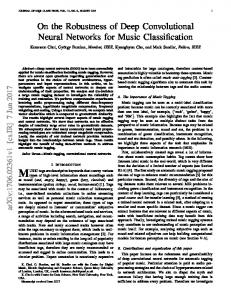
Figure 3. CNN analysis showing car coordinates (x, y), IOU (z), and confidence (color).

tion within few evaluations on the real system. Since we search for counterexamples, i.e, samples where the score returned by the neural network is low, we use GP-Lower Confidence Bound (GP-LCB) as our objective function. Since the optimal sample u∗t is not known a priori, the optimal strategy has to balance learning about the location of the most falsifying sample (exploration), and selecting a sample that is known to lead to low scores (exploitation). We formulate the objective function as, ut = 1/2 argminu∈U µt−1 (u) − βt σt−1 (u) where βt is a constant which determines the confidence bound. 2.4. Visualization We now show how the gathered information can be visualized and interpreted. In our data analysis, we consider two factors: the confidence score and the Intersection Over Union (IOU) that is a metric used to measure the accuracy of detections. IOU is defined as the area of overlap over the area of the union of the predicted and ground-truth bounding boxes. Our visualization tool associates the center of the car of the generated images to the confidence score and IOU returned by the treated CNN. Fig. 3 depicts some examples where the x and y are the center coordinates of the car, z is the IOU, and the color represents the CNN confidence score. We also offer the possibility to superimpose the experimental data on the background used to render the pictures (see Fig. 4). In this case, the IOU is represented by the dimension of the marker. This representation helps us to identify particular regions of interest on the road. In the next section, we will see how these data can be interpreted.

3. Implementation and Evaluation We implemented the presented framework in a tool available at https://github.com/shromonag/ FalsifyNN. The tool comes with a library composed by a dozen of road backgrounds and car models, and it interfaces to the CNNs SqueezeDet (Wu et al., 2016), Kit-

(b) Yolo. Figure 4. Superimposition of the analysis on road background.

tiBox (Teichmann et al., 2016), and Yolo (Redmon et al., 2016). Both the image library and CNN interfaces can be personalized by the user. As an illustrative case study, we considered a countryside background and a Honda Civic and we generated 1k synthetic images using our rendering techniques (Sec. 2.2) and the Halton sampling sequence (Sec. 2.3). We used the generated pictures to analyze SqueezeDet (Wu et al., 2016), a CNN for object detection for autonomous driving, and Yolo (Redmon et al., 2016), a multipurpose CNN for realtime detection. Fig. 3 displays the center of the car in the generated pictures associated with the confidence score and IOU returned by both SqueezeDet and Yolo. Fig. 4 superimposes the heat maps of Fig. 3 on the used background. There are several interesting insights that emerge from the graphs obtained(for this combination of background and car model). SqueezeDet has, in general, a high confidence and IOU, but has a blind spot for cars in the middle of the road on the right(see the cluster of blue points in Fig. 3(b) and 4(a)). Yolo’s confidence and IOU decrease with the car distance (see Fig. 3(b)). We were able to detect a blind area in Yolo, corresponding to cars on the far left (see blue points in Fig. 3(b)). Note how our analysis can be used to visually compare the two CNNs by graphically highlighting their differences in terms of detections, confidence scores, and IOUs. A comprehensive analysis and comparison of these CNNs should involve images generated by combinations of different cars and backgrounds. However, this experiment already shows the benefits in using the presented framework and highlights the quantity and quality of information that can be extracted from a CNN even with a simple study.

Systematic Testing of Convolutional Neural Networks for Autonomous Driving

References Aly, Mohamed. Real time detection of lane markers in urban streets. In Intelligent Vehicles Symposium, IV, pp. 7–12. IEEE, 2008. Bojarski, Mariusz, Testa, Davide Del, Dworakowski, Daniel, Firner, Bernhard, Flepp, Beat, Goyal, Prasoon, Jackel, Lawrence D., Monfort, Mathew, Muller, Urs, Zhang, Jiakai, Zhang, Xin, Zhao, Jake, and Zieba, Karol. End to end learning for self-driving cars. CoRR, abs/1604.07316, 2016. URL http://arxiv.org/ abs/1604.07316. Dougherty, Mark. A review of neural networks applied to transport. Transportation Research Part C: Emerging Technologies, 3(4):247–260, 1995. Dreossi, Tommaso, Donz´e, Alexandre, and Seshia, Sanjit A. Compositional falsification of cyber-physical systems with machine learning components. In NASA Formal Methods Symposium, pp. 357–372. Springer, 2017. Geiger, Andreas, Lenz, Philip, Stiller, Christoph, and Urtasun, Raquel. Vision meets robotics: The kitti dataset. International Journal of Robotics Research, IJRR, 2013. Goodfellow, Ian, Pouget-Abadie, Jean, Mirza, Mehdi, Xu, Bing, Warde-Farley, David, Ozair, Sherjil, Courville, Aaron, and Bengio, Yoshua. Generative adversarial nets. In Advances in neural information processing systems, pp. 2672–2680, 2014. Halton, John H. On the efficiency of certain quasi-random sequences of points in evaluating multi-dimensional integrals. Numerische Mathematik, 2(1):84–90, 1960. Huang, Xiaowei, Kwiatkowska, Marta, Wang, Sen, and Wu, Min. Safety verification of deep neural networks. arXiv preprint arXiv:1610.06940, 2016. Katz, Guy, Barrett, Clark, Dill, David, Julian, Kyle, and Kochenderfer, Mykel. Reluplex: An efficient smt solver for verifying deep neural networks. arXiv preprint arXiv:1702.01135, 2017. Kong, Hui, Audibert, Jean-Yves, and Ponce, Jean. Vanishing point detection for road detection. In Computer Vision and Pattern Recognition, CVPR, pp. 96–103. IEEE, 2009. Niederreiter, Harald. Low-discrepancy and low- sequences. Journal of number theory, 30(1):51–70, 1988. Papernot, Nicolas, McDaniel, Patrick, Jha, Somesh, Fredrikson, Matt, Celik, Z Berkay, and Swami, Ananthram. The limitations of deep learning in adversarial settings. In Security and Privacy (EuroS&P), 2016 IEEE European Symposium on, pp. 372–387. IEEE, 2016.

Redmon, Joseph, Divvala, Santosh, Girshick, Ross, and Farhadi, Ali. You only look once: Unified, real-time object detection. In Computer Vision and Pattern Recognition, CVPR, pp. 779–788, 2016. Sobol, Ilya M. Uniformly distributed sequences with an additional uniform property. USSR Computational Mathematics and Mathematical Physics, 16(5):236–242, 1976. Szegedy, Christian, Zaremba, Wojciech, Sutskever, Ilya, Bruna, Joan, Erhan, Dumitru, Goodfellow, Ian, and Fergus, Rob. Intriguing properties of neural networks. arXiv preprint arXiv:1312.6199, 2013. Teichmann, Marvin, Weber, Michael, Z¨ollner, J. Marius, Cipolla, Roberto, and Urtasun, Raquel. Multinet: Real-time joint semantic reasoning for autonomous driving. Computing Research Repository, CoRR, abs/1612.07695, 2016. URL http://arxiv.org/ abs/1612.07695. Wu, Bichen, Iandola, Forrest, Jin, Peter H., and Keutzer, Kurt. Squeezedet: Unified, small, low power fully convolutional neural networks for real-time object detection for autonomous driving. 2016.