TA

The role of the Alula in avian flight and it’s application to small aircraft: a numerical study Die Funktion der Alula im Vogelflug und ihr bionisches ¨ kleine Flugmaschinen: Potential fur Numerische Untersuchungen

Master’s thesis submitted by: student ID: course: first examiner: second examiner: date:

Aljoscha Sander 322128 Biomimetics: Mobile Systems Prof. Dr. Albert Baars Prof. Dr. Eize Stamhuis 23rd of July, 2018

”Die Macht des Verstandes, o, wend’ sie nur an, [. . . ] Sie wird auch im Fluge Dich tragen!” - Otto Lilienthal, Der Vogelflug als Grundlage der Fliegekunst, Berlin, 1889, p. 149

Declaration of Authorship I declare that this thesis and the work presented in it are my own and has been generated by me as the result of my own original research. No other person’s work has been used without due acknowledgement and where I have quoted from the work of others, the source is always given. With the exception of such quotations, this thesis is entirely my own work. None of this work has been published before submission.

Bremen, Place, Date

Signature

Acknowledgement & Dedication This thesis would not have been possible if not for a lot of people, first and foremost my parents. Therefore I dedicate this work to: Tamara & Gerd Sander Prof. Dr. Kesel has made it possible to do all this in the first place. Prof. Dr. Baars was and is an incredible supervisor demanding, not by exerting pressure but by feeding my thrive for perfection. Prof. Dr. Stamhuis is the sceptic with the blinking eye, making sure I would not loose track of ’the story’ while embarking on numerical adventures. Additionally he warranted me access to the computational facilities in Groningen. Thank you! The computational facilities in Groningen are maintained by a superb group of administrators, without them none of the simulations would have worked in the first; place. A special thank you goes out to Bob Dröge who managed get OpenFOAM compiled on the peregrine cluster. A big thank you to all the people who helped me getting this thesis into the structured and printed version it is now; especially Carolina, Felix, Lea, Lena, Lukas and Vincent. To my wife, Carolina: thank you for enduring my obsession with birds, computers & aerodynamics.

Thanks to everyone participating in open-source projects - this study is based entirely on open-source software -

Abstract The Alula, a small set of feathers located at the leading edge of avian wings in between the arm and hand wing has long baffled scientist as to it’s function. Here, by means of computational fluid dynamics a simplified Alula in both gliding and flapping flight conditions is investigated at a wing Reynolds number of 20,000. A simple 3D wing geometry from literature is used. Results from gliding flight conditions show an increase in both lift and drag as well as a significantly altered pitching moment. A reduction in adverse pressure gradient results in a reduction of separation. Furthermore, the formation of an Alula tip vortex and at high angles of attack a Alula leading edge vortex can be observed. The latter only emerges if the Alula is deflected in a fashionable manner. Both vortices are advantageous to the reduction in separation. In flapping flight no influence of the Alula onto forces or flow topology can be observed, since flow is dominated by the formation of a leading edge vortex in the main wing. A technical abstraction of the Alula as a novel flow control device for low Reynolds number flow is presented. In future studies influence of Alula geometry, orientation and the influence of Reynolds number should be investigated. Keywords: Alula, CFD, flow control, gliding flight, flapping flight Zusammenfassung ¨ Am Ubergang zwischen Hand- und Armschwinge findet sich bei den meisten Vögeln eine Ansammlung von kleinen Federn: die Alula. Die mögliche aerodynamische Funktion der Alula wurde bisher nicht eindeutig aufgeklärt. Im Rahmen dieser Arbeit wurde mittels numerischer Strömungssimulation eine vereinfachte Geometrie der Alula bei einer Reynolds-Zahl von 20.000 sowohl in Gleit- als auch ¨ wurde eine Geometrie aus der Literatur genutzt. Im Schlagflugkonditionen untersucht. Als Flugel Gleitflug konnte eine Zunahme von Auftriebs- und Widerstandskraft, als auch positivem Nickmoment beobachtet werden. Im Nachlauf der Alula sorgt die Reduktion des Druckgradient in Strömungsrich¨ eine reduzierte Wahrscheinlichkeit der Strömungsablösung. Zusätzlich konnte die Ausbildung tung fur eines Spitzenwirbels und bei hohen Anstellwinkeln eines Vorderkantenwirbels an der Alula beobachtet werden. Beide Wirbel tragen zu einer Reduktion der Strömungsablösung bei. Im Schlagflug konnte keinerlei Einfluss der Alula auf Kräfte oder Strömungstopologie festgestellt werden. Dies ist wahrschein¨ im Schlagflug zuruck ¨ zu fuhren. ¨ lich auf die Dominanz des Vorderkantenwirbels am Flugel Eine mögliche ¨ kleine Reynoldtechnische Abstraktion der Alula als eine neue Methode zur Strömungskontrolle fur ¨ szahlen wurde aufgezeigt. In zukunftigen Arbeiten sollte der Einfluss der Geometrie, der Orientierung ¨ und der Einfluss der Reynolds-Zahl untersucht werden. der Alula im Bezug auf den Flugel

ix

Contents 1

Introduction 1.1 Avian flight . . . . . . . . . . . . . . . . . . . . . . . . . . . . . . . . . . . . . . . 1.2 Alula . . . . . . . . . . . . . . . . . . . . . . . . . . . . . . . . . . . . . . . . . . 1.3 Scope of thesis . . . . . . . . . . . . . . . . . . . . . . . . . . . . . . . . . . . . . .

1 1 8 11

2

Material and Methods 2.1 Geometry and Kinematics . . . . . . . . . . . . . . . . . . . . . . 2.2 Numerical Setup . . . . . . . . . . . . . . . . . . . . . . . . . . 2.2.1 Description of Simulations . . . . . . . . . . . . . . . . . 2.2.2 Normalisation and Characterisation . . . . . . . . . . . . 2.2.3 Model Equations . . . . . . . . . . . . . . . . . . . . . . 2.2.4 Computational Domain, Initial- and Boundary Conditions 2.2.5 Discretisation . . . . . . . . . . . . . . . . . . . . . . . . 2.2.6 Algorithms and Solvers . . . . . . . . . . . . . . . . . . . 2.2.7 Implemented Simulations & Post-Processing . . . . . . . .

. . . . . . . . .

. . . . . . . . .

. . . . . . . . .

. . . . . . . . .

. . . . . . . . .

. . . . . . . . .

. . . . . . . . .

. . . . . . . . .

. . . . . . . . .

. . . . . . . . .

13 13 15 15 16 18 19 22 26 27

3

Results 3.1 The Alula in Gliding Flight . 3.1.1 Forces . . . . . . . . 3.1.2 Flow Topology . . . 3.1.3 Turbulence . . . . . 3.2 The Alula in Flapping Flight 3.2.1 Forces . . . . . . . . 3.2.2 Flow Topology . . .

. . . . . . .

. . . . . . .

. . . . . . .

. . . . . . .

. . . . . . .

. . . . . . .

. . . . . . .

. . . . . . .

. . . . . . .

. . . . . . .

. . . . . . .

. . . . . . .

. . . . . . .

. . . . . . .

. . . . . . .

. . . . . . .

. . . . . . .

. . . . . . .

. . . . . . .

29 29 29 34 39 41 41 44

4

Discussion 4.1 Low Reynolds Airfoil Flow & Robustness of Results 4.2 The Alula in Gliding Flight . . . . . . . . . . . . . 4.2.1 Forces, Flow topology & Turbulence . . . . 4.2.2 Cause and Effect . . . . . . . . . . . . . . 4.3 The Alula in Flapping Flight . . . . . . . . . . . . 4.3.1 Forces, Flow Topology & Turbulence . . .

. . . . . .

. . . . . .

. . . . . .

. . . . . .

. . . . . .

. . . . . .

. . . . . .

. . . . . .

. . . . . .

. . . . . .

. . . . . .

. . . . . .

. . . . . .

. . . . . .

. . . . . .

. . . . . .

. . . . . .

. . . . . .

47 47 52 52 57 64 64

5

Conclusion 5.1 Numerical Modelling . . . . . . . . . . . . . . . . . . . . . . . . . . . . . . . . . . 5.2 Avian Flight . . . . . . . . . . . . . . . . . . . . . . . . . . . . . . . . . . . . . . . 5.3 Potential Application . . . . . . . . . . . . . . . . . . . . . . . . . . . . . . . . . .

67 67 67 70

References Appendix

. . . . . . .

. . . . . . .

. . . . . . .

. . . . . . .

. . . . . . .

. . . . . . .

. . . . . . .

. . . . . . .

. . . . . . .

. . . . . . .

. . . . . . .

71 i

xi

Contents

Abbreviations ALEV ATV CAD DNS LES LEV LIC OpenFOAM PIMPLE PISO PIV RANS SGS UAV WALE-model WTV

Alula Leading Edge Vortex Alula Tip Vortex Computer-Aided Design Direct Numerical Simulation Large Eddy Simulation Leading Edge Vortex Line Integral Convolution Open Source Field Operation and Manipulation Pressure-Implicit Merge PISO SIMPLE Pressure-Implicit with Splitting of Operator Particle Image Velocimetry Reynolds Averaged Navier Stokes Sub-Grid Scale Unmanned Aerial Vehicle Wall-Adapted Local Eddy-Viscosity Wing Tip Vortex

xiii

Contents

Nomenclature A D f k L p R Re Ro S St T u V v ρ

xiv

Flapping amplitude Drag force Flapping frecuency Reduce frequency Lift force Pressure Half wing span, flapping radius Reynolds number Rossby number Spanwise force Strouhal number Thrust Flow velocity Wing tip velocity Dynamic viscosity Density

1

Introduction

In this chapter an overview of avian flight research is given with a short excursus to definitions & nondimensional parameters. The Alula is introduced and the various theories as to it’s function are explained. The chapter ends with the scope of thesis and a set of working hypotheses.

1.1 Avian flight The beginning of humankinds desire to fly is long lost in the midst of time. Flying has played a - often crucial and esoteric - role in humankinds legends & tellings. From the ancient egyptians (Etana flying birdlike (Horowitz 1998, p.53)), greek mythology (Daedalus and Icarus, (Ovid 0008)) to the broomriding witches of the middle ages (Bauer and Behringer 1997), human flight remained an unmet desire, only mastered by gods or supernatural powers. Leonardo DaVinci was among the first to pursue this dream by methodically analysing the flight of birds and drafting a variety of flying machines. However, none were built and his work was lost for his predecessors until much later. With the upcoming of the modern sciences - including fluid dynamics - flying became more of a practical problem. Progress with lighter-than-air vehicles was achieved (most notably in france, e.g. the brothers Montgolfiere), closely followed by a trail of utterly fearless pioneers, who tried to proof they had conquered flying by jumping off roofs, towers, cliffs and later on balloons. It wasn’t before the late 19th century that substantial achievements were made. Otto Lilienthal and his highly regarded monogram Der Vogelflug als Grundlage der Fliegekunst (Lilienthal 1889) are among the most noteworthy. While Lilienthal pursued manned flight, he explicitely used avian flight as a basis for his aircraft designs. Among the many he build, the common characteristic is the natural, organic design of the wings, as opposed to many other wing designs from the late 19th and early 20th century. While Lilienthal realized that the curvature of wing profile is crucial to force production - most notably the lift force - no explanation as to why was available. To understand avian flight, a glance at the general anatomy of a bird is necessary. Figure 1.1 shows a schematically drawn, generalized bird. On the left hand side, feathers (only primaries and secondaries), wing bones and the Alula are shown. On the right hand side, geometrical properties relevant to aerodynamics are depicted. Figure 1.2 shows forces and moments acting on a bird during flight (subfigure A). Uplifting force is regarded as lift force L, force in streamwise direction as drag force D and force acting perpendicular to both L and D is referred to as transversal force. Clockwise rotation around the lift force axis is denoted as yawing, clockwise rotation around drag force vector as rolling and clockwise rotation around transversal force vector as pitching. Subfigure B illustrates a flapping motion from a frontal perspective. Aerodynamically relevant parameters are the flapping frequency f, the flapping amplitude A, flapping radius R and the wing tip velocity V. The motion of a wing is cyclic, also denoted as stroke cycle, and can be divided into two phases per cycle: upstroke and downstroke. In the downstroke, the wing tip moves from dorsal to ventral describing a downwards motion in the frame of reference of the bird. The contrary applies to the upstroke. Both are depicted in Figure 1.3.

1

1 Introduction

Span S

Alula

Ulnare Radius

Wing area A l

Humerus

C

C

Primary �eathers Secondary �eathers

Figure 1.1: Schematic drawing of a generalised bird from frontal and top view. Illustration partially adapted from Pennycuick (2007). On the upper side the frontal view shows the wing span S. In the top view on the left hand side the primary and secondary feathers are depicted as well as the Alula. Additionally the bones that make up the wing skeleton are shown (Humerus, Ulnare & Radius). On the right hand side of the top view, geometric properties relevant for fluid dynamics are shown (planform wing area A, single wing span l, maximum chord length C and average chord length C.

Observing birds led to a variety of theories in order to explain both flapping and gliding flight. For gliding flight it was already known, that a flat plate under an angle of attack with respect to the flow vector generated a resulting force with an angle roughly perpendicular to the mean flow direction (assuming a small angle of attack). From Bernoulli’s equation it was established, that the aerodynamic forces scale with dynamic pressure (p = 0.5 · ρ · u2 where u is the velocity and ρ the density of the fluid). Applying this knowledge to flapping flight yielded a considerable deviation between the velocities observed in free flying birds and theoretical values. Furthermore, calculating the power required to keep birds aloft resulted in power densities (Watts per kg muscle) exceeding those of humans and horses by half an order of magnitude (Fitzgerald 1898). Different models were developed to explain the differences between observations and theory. Fitzgerald and Fitzgerald (1909) propagated the theory of a weightless mass that is shed into the wake and thus provides momentum (lift and drag) which drives the bird’s motion. However, this theory would require a bird’s wing to always have a greater local velocity than the oncoming fluid which is clearly not the case. Fullerton (1925) compared birds to airplanes, drawing the conclusion, that if treated as such, explaining lift, drag, thrust and power output is feasible and yields realistic results. He specifically explains, that wings, both generating thrust and lift must maintain a intricate balance between all forces to enable flapping flight. He observed, that both drag force and wing camber change with flight velocity and that the flexibility of the wing probably plays an important role. Walker (1925)

2

1.1 Avian flight

A

B Lift Yawing

R

Upstroke A

V Downstroke

Drag Rolling

Uc

Transverse Pitching

∝ 2πf

t

Uc

Figure 1.2: Schematic drawing of forces and moments acting on a airborne bird (A) and a simplified flapping cycle (B). During flight a bird must overcome drag to make headway and generate lift to stay aloft. Transversal forces cancel out as long as a symmetric kinematic pattern is applied and the bird moves parallel to oncoming flow. The force induce moments along at the center of gravity which must be controlled by the bird in order to maintain control. Important parameters during flapping are the tip-to-tip amplitude A, wing velocity V, Radius R, fluid velocity Uc and the flapping frequency f. Illustration in (B) partially adapted from Pennycuick (2007).

re-analysed the hitherto current theories including Fullerton (1925), successfully identified their shortcomings and gave a first estimate for both lift and drag forces as a function of the dynamic pressure. He identified the ratio k between the fluid velocity U (e.g. relative velocity of the bird with regards to wind speed) and the vertical wing velocity V and noted that most birds fly within a range of k=

V = 0.3 .. 0.42 U

(1.1)

This relation today can be found in the Strouhal number: St =

f ·l U

(1.2)

where f is the flapping frequency, l a characteristic length (for flapping flight the tip-to-tip amplitude A) and U the fluid velocity (see Figure 1.2 for details). Based upon the angles of attack observed on the wings of various birds, Walker (1925) concluded, that the inner wing with the angle of attack being positiv in both up and downstroke is mostly responsible for generating lift force, while the outer part of the wing produces thrust (though mostly during downstroke). He estimates, that for a given bird with a velocity U and wing area A moving in a fluid with viscosity ρ, lift force is proportional to L = 0.3 · AρU 2 and drag force D = 0.04AρU 2 . While the estimates are not completely off, no mechanism explaining the force generation on a flapping wing was presented. While biologists were puzzled by the power expenditure, the fluid dynamicists of the time were busy figuring out the same phenomenon in the context of airplanes. One striking effect was the observation that lift force is not instantaneous, but requires a certain amount time, which can be expressed in number of chord lengths travelled when taking off in an airplane. Wagner (1925) used the third Helmholtz theorem in conjunction with potential flow theory to develop a mathematical formulation describing the number of wing chord lengths needed until the lift force of a wing with a given geometry moving in a fluid with a density ρ reached a asymptotic state ( > 80%L). Today this is regarded as Wagner’s theorem. However, this went by unnoticed by the biologists.

3

1 Introduction

Upstroke V

α

Downstroke

A

UREL

α

UREL Uc

Uc

L

C

R

W

V

R

D

Uc

B

L

D

T

Uc

W

Figure 1.3: Schematically drawn flapping cycle in forward flight. Depicted are upstroke (A & C) as well as downstroke (B & D). In the upper row wing (V) and fluid (Uc ) velocity which determine the induced angle of attack (α) between relative velocity vector UREL and geometrical angle of attack are depicted. In the bottom row, forces acting on the wing and thus on the bird are shown. Lift (L) is generated during both up and downstroke while thrust (T) only occurs during downstroke. Lift (L) and drag (D) are the components of the resulting force (R). Additionally the weight force W is shown. Illustration of flapping cycle adapted from Lilienthal (1889).

Lorenz (1933) described in detail the flight of different types of birds and divided the aerial locomotion of birds into four different categories: gliding, soaring, flapping and hovering. He then formulated the theory, that lift force stems from the change in potential energy of the bird. He proposed, that at each downstroke, a bird would increase it’s potential energy by pushing itself off the air (and thus increasing it’s altitude by a fraction) and then gliding forwards in the upstroke to reach it’s previous altitude. While the observation that the center of mass of a bird in flapping flight does indeed oscillate around the mean pathline is correct, the conclusion drawn from it is not. It wasn’t until 1937 (Stolpe and Zimmer 1937) that the connection between pressure (and thus lift), which was well established in (airplane) engineering and the flapping flight of birds was made. The authors measured the pressure on both upper and lower side of a stuffed avian wing in a wind tunnel, which resulted in a pressure difference between lower and upper side of the wing of roughly 3 - 4 x the dynamic pressure. They discarded the idea of the bird shedding a mass (weightless or not) and thus generating momentum for forward flight. Holst and Kuchemann (1942) then compared structures that can be found in the wings of birds, such as the Alula, slotted wing tips, forked tails and the rise of plumage at high angles of attack (self actuating flaps) with technical solutions, developed for airplanes.

4

1.1 Avian flight As a measure to compare avian flight with the flight of (then) modern airplanes, the authors introduced the Reynolds number: lc · u (1.3) ν Where lc is a characteristic length scale (for a wing the chord length c), u the flow velocity and ν the dynamic viscosity. This number represents the ratio of inertial to viscous forces and was first established by Stokes (1850) 1 . Comparing, however, was hard at this point since very little data on the dependence of flow phenomena on the Reynolds number (except of course the transition from laminar to turbulent flow) was available. A few studies, such as Millikan and Klein (1933) started to examine Reynolds number effects, but these studies were mostly done in an engineering context. Holst and Kuchemann (1942) also concluded in flapping flight for Strouhal numbers smaller than St < 0.2 the influence of the flapping motion onto the flow should be negligible and the flapping wing could be treated as if in gliding motion. A short digression to emphasize the importance of the Reynolds number (Equation 1.3) must be made. For a simple geometric object such as a cylinder with a characteristic length c moving through fluid with a dynamic viscosity ν at a velocity of U flow detaches from the surface for Re > 5, becomes periodically transient for Re > 100 and turbulence can emerge for Re ≥ 10, 000. For slender bodies such as wings these characteristic Reynolds numbers are similiar, though in general corresponding phenomena occur at high values for Re. Flow is therefore subdivided into Reynolds number regimes. In the scope of airfoils, Lissaman (1983) defines the low-Reynolds number regime as Re < 70, 000. This definition is adapted within this thesis. Until 1951 very few new insights were generated (Brown 1951), which was partly due to the complexity of flapping flight. Progress was made when the taste for entertainment led to the development of high quality cameras, which were in turn used by Brown (1953) to examine the kinematics of a pigeon in different states of flapping flight. The data allowed for a precise description of the ”average” flapping flight cycle at different velocities and thus led to a detailed understanding of the relative motions involved during the flapping cycle. More and more studies followed, resulting in 4 categories of flyers (Savile 1957) based on flight behaviour and the correlating wing geometry: Re =

• Elliptical wing: A wing specifically evolved for species living in confined spaces. • High speed wing: Found in birds that spend most of their life airborne. • High aspect ratio wing: A type of wing mostly found in sea birds (dynamic gliding). • Slotted high lift wing: A wing found in soaring predators. The utilisation of wind tunnels in conjunction with live animals (Pennycuick 1960), as well as field observations (Newman 1958; Pennycuick 1983; Tucker and Parrott 1970; Withers 1979) brought new insights into flapping flight. With a deeper understanding of the mechanical aspects involved, questions concerning power expenditure and flight control emerged. Brown (1963) proposed - based upon observations of live animals - the following interrelation between attitude control and flight kinematics (for definitions of motions, see Figure 3.10).

1 Though

it was not referred to as the Reynolds number. Reynolds (1894) used the ratio as a measure to describe the state of flow (laminar, transitional or turbulent) in a pipe. It was Arnold Sommerfeld, the physician who introduced the name ”Reynolds number”

5

1 Introduction • Pitching: The pitching motion, most important during landing and hovering is controlled by pitching tail feathers up (dorsal) and down (ventral). • Rolling: The rolling motion is mostly controlled by changing the amplitude of the flapping wing (as opposed to changing the flapping frequency). • Yawing: Asymmetries in the tail in combination with pitch control can lead to a yawing motion. The advances in observations and experiments were accompanied by half-empirical, half-theoretical models, such as Rayner (1979). Those models are generally referred to as quasi-steady models. The basic assumption is, that ”the instantaneous aerodynamic forces on a flapping wing are assumed to be identical with those which the wing would experience in steady motion at the same instantaneous speed and angle of attack” (Ellington 1984). However, while these models provide accurate predictions for a wide range of use cases, there are specific cases where fluid dynamics phenomena, such as vortex shedding, play a role in the generation of aerodynamic forces that cannot be captured by these approaches. Ellington (1984) presented cases of hovering flyers where quasi-steady models failed to capture forces accurately. Based on additional experiments the author argues that there are probably cases in flapping flight where the models will fail. Rayner (1985) showed that some birds do not flap continuously and while doing so there are generally two different flight modes: flapping and gliding both with wings extended or flapping with extended wings and gliding with wings retracted. This was followed by Spedding (1987), who showed that a system of interconnected vortices can be found in the wake of a flapping Kestrel and by thus providing first experimental evidence of tip vortices in bird flight. The forces generated are dependent on wing span, which is connected to the vortex wake by induced drag (Tucker 1987). Attention shifted to a broader view onto flapping flight and it’s implications for ecological and migratory performance as well as behavioural adoptions necessary for enabling long distance flapping flight (Hedenström 1993; Hedenström and Alerstam 1992; Rayner 1990). In this context Tucker (1993) provided experimental evidence that slotted wing tips, as can be observed in many soaring birds greatly reduce drag and thereby increase the lift-to-drag ratio. As an additional energetic cost inertial forces due to wing mass were identified and calculated by Berg and Rayner (1995) (≈ 15% of power are devoted to inertial forces of the wing). They showed that the inertial forces Fi scale with body mass m: Fi ∝ m0.799 . In parallel Ellington et al. (1996) provided an explanation for force production in insects which static aerodynamics failed to explain: during flapping a vortex is formed at the leading edge of the wing (Leading Edge Vortex, LEV). However, this phenomenon was only shown for small Reynolds numbers (Re < O(103 )). Hall and Hall (1996) tried to identify minimum power requirements for flapping flight and provided a inverse relation between power requirements for lift and drag force production, suggesting the existence of optimal flight speed depending on flight kinematics. With the previously mentioned upcoming of trained birds in wind tunnels, Pennycuick et al. (1996) showed that interactions between wing and body result in much lower drag contribution of the body in flapping flight than when measuring wing and body seperately. Tobalske and Dial (1996) showed that in order to achieve different flight speeds in magpies and pigeons the animals alter the stroke and body plane angles & wing tip trajectory while maintaining a constant flapping frequency which corresponds well to the physiological power constrains due to inertial forces. The authors identify two different gaits which correspond either to the shedding of closed vortex rings or the formation of a continuous vortex street. Later, Tobalske (2000) showed that the vortex patterns correspond to two fundamentally different upstroke patterns: in slow flight the wing is pronated at the beginning of the upstroke while up and downstroke take place in the same plane. This is regarded as tip reversal. At higher speeds the wing tip moves towards the aft during upstroke while the wing no longer rotates around its main axis. This flapping pattern corresponds to the

6

1.1 Avian flight creation of a continuous vortex street and is denoted as feathered upstroke (later also named swept-wing upstroke). Meanwhile, Berg and Ellington (1997) provided evidence for the existence of a LEV at higher Re. Sane and Dickinson (2002) presented a revised quasi-steady model for flapping flight which incorporated rotational effects. Stability of both gliding and flapping flight was analysed by Taylor and Thomas (2002) and Thomas and Taylor (2001). The authors argued that while it seems intuitively contradictory, flapping flight can actually result in a stabilisation of the bird, though the upstroke might cause momentary instabilities. Hedrick et al. (2004) ascribed 14 % of total lift to the upstroke in cockatiels. Nudds et al. (2004) provided circumstancial evidence that the evolution of wings is driven by fluid dynamic efficiency, linking Strouhal numbers of 0.21 ≤ St ≤ 0.25 to 90 % of birds. Usherwood and Ellington (2002) and Birch (2003) systematically investigated the effects of LEVs at different Re providing experimental proof of the LEV being responsible for a significant increase in both lift and drag forces. Birch et al. (2004) then proved the existence of LEVs on flapping wings at Re ≈ O(103 ). The existence of LEVs in gliding swifts was first described by Videler et al. (2004). The authors linked the performance of gliding swifts to the sweeping angle which at lower angles of attack resulted in LEVs at Re = O(104 ). Lentink et al. (2007) then showed that the gliding performance in swifts is controlled by changing the sweeping angle. Finally the existence of LEVs in flapping flight at Re = 6000 was shown by Shyy and Liu (2007), linking transient force generation and the existence of LEVs. A measure to predict the stability of a LEVs is the Rossby number (Ro), the ratio between centripetal and Coriolis acceleration. The concept was introduced to bio-fluid-mechanics by Lentink and Dickinson (2009b) and applied to a broad range of data by Lentink and Dickinson (2009a). The link between Rossby number & stability of vortices can also be found in Devenport et al. (1996) though it originates back to Spall et al. (1987) where Ro is defined as the ratio between axial and tangential flow velocity (in a vortex bound coordinate system) and for values Ro > 1 vortices may break down. Lentink and Dickinson (2009a) fitted the Rossby number to flapping flight and to consider forward velocity linked it with the advance ratio J : J=

U∞ 4Af

(1.4)

R (1.5) c Where U∞ is forward velocity, A tip-to-tip amplitude, f flapping frequency, R flapping sweeping radius and c mean chord length. For hovering flight J = 0 and Ro collapses to the aspect ratio AR = R/c. Based on experimental results, the authors argue that for Ro > 4 the leading edge vortex becomes unstable and diminishes. This was criterion was picked up by Hubel and Tropea (2010) who conducted flapping flight experiments of a duck mockup at Re ≈ O(105 ). LEVs formed but became unstable and diminished over the wing span. Thielicke (2014) conducted extensive experiments with a simple flapping device, investigating the influence of wing geometry & St on LEVs. The author showed, that a thin wing enhances the build-up of a LEV. LEVs were found for all St and geometries. In a recent review, Chin and Lentink (2016) concluded that while aerodynamics of insects are fairly well understood many aspects of bird aerodynamics, whether in hovering, slow flapping or fast flapping are still lacking understanding or proof. Ro =

q

(J 2 + 1)

7

1 Introduction

1.2 Alula In most birds at the intersection of arm and hand wing a small set of feathers can be found: the Alula (see Figure 1.1, arrows).

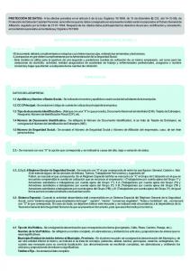
Figure 1.4: Gull gliding in strong updraft with Alula extended. The photo was taken on a ferry, where strong sidewinds induced a updruft at the windward ship’s side. Gulls, on the lookout for possible food were accompanying the ferry with no apparent flapping of wings, maintaining heading and speed by adjustment of wings positions.

These feathers connect to a bone, reminiscence of what is evolutionarily left of the thumb. It possess two translational and one rotational degree of freedom (abduction and adduction: yawing with respect to the leading edge, tilting both up and downwards and pronation & supination). Alternative names are wrist slot (Graham 1932), bastard wing (Videler 2005) or thumb-inion (Holst and Kuchemann 1942). The Alula is between 10 % and 30 % wing span in size and is most prominent in pigeons, gulls and crows (Lee and Choi 2017). It is hardly visible, since the Alula is completely attached to the leading edge most of the time. Its function however is controversial; to most authors, its function is that of a spoiler increasing lift and reducing drag by manipulating flow topology. Graham (1932) proposed that it functions as a slat, then known as a Handley-Page auxiliary airfoil. This type of leading edge device is widely used in aerodynamic engineering. Slats only slightly increase the slope of the lift coefficient curve but extend the critical angle of attack at which flow separation may occur. This is achieved by reducing the adverse pressure gradient over the main wing (Sadraey 2013). Savile (1957) showed a strong correlation between high-lift flight conditions (takeoff, landing, soaring/gliding with an high angle of attack) and the (visible) appearance of the Alula during flight manouvers. This behaviour was confirmed for different birds in different flying states such as gliding flight in the Fulmar petrel (Pennycuick 1960), soaring flight in the black vulture (Newman 1958), flapping flight in pigeons (Pennycuick 1968) and flapping and gliding in the andean condor (McGahan 1973a; McGahan 1973b). Nachtigall and Kempf (1971) came to a similar conclusion as Graham (1932) for gliding flight. By visualising the flow between Alula and leading edge in prepared stuffed wings, they showed that the flow detached closer to the trailing edge than without Alula. By measuring lift and drag for a wide range of angles of attack, they showed an increase in lift of up to 25 %. Furthermore, they hypothesised that the Alula might increase pitching moment at large angles of attack to allow for a greater turn rate when perching. Brown and Fedde (1993) postulated that the Alula serves as an airflow sensor as opposed to being a control surface of the wing.

8

1.2 Alula ´ A first systematic description of Alulae was published by Alvarez et al. (2001), who also reported, that the Alula most probably has no active influence onto the flow and is being peeled off passively from the bird’s wing leading edge due to pressure gradients. This is in stark contrast with the 3 degrees of freedom that can be controlled actively by the bird. Meseguer et al. (2005) showed in wind tunnel experiments, that a wing equipped with an artificial Alula leads to a maximum increase in lift of 17%. While the evidence of the Alula serving as a control surface became stronger, no explanation as to the physical effect leading to a significant increase in forces was presented. Videler (2005) proposed the idea, that instead of working as a slat, the Alula might seperate hand and arm section of the avian wing and thus reduce separation & increase lift. In aerodynamic engineering, this type of device is regarded as a boundary layer fence and has been widely used in modern aircraft. Austin and Anderson (2007) conducted wind tunnel experiments on prepared bird wings. For only one species significant increase in lift was found. Observation-based evidence of the Alula serving a particular role in perching was presented by Carruthers et al. (2007) and Carruthers et al. (2010) for a steppe eagle. They concluded that the Alula works as a strake a type of control surface inducing a vortex that leads to stabilisation of the flow and in this case increases the stability of the LEV forming on the hand wing of the specimen. Interestingly the authors proposed, that the Alula is peeled of the leading edge of the wing passively by a pressure gradient and only after passive deployment an active control of it’s position relative to the wing is executed.

9

1 Introduction New data presented by Lee et al. (2015) supports a first explanation of the means of flow manipulation: using Particle Image Velocimetry (PIV) experiments the authors showed that a small chordwise vortex, spawned by the tip of the Alula can be observed under gliding flight conditions Figure 1.5. ATV

A Uc

C B

Alula

Alula tip vortex (ATV)

Figure 1.5: Schematic representation of the Alula tip vortex (ATV), a phenomenon first described by Lee et al. (2015). In the upper part of the figure (A), a frontal view is shown, in the lower part the corresponding top view (B) and in (C) the side view. The Alula is annotated with arrows. The ATV forms at the tip of the Alula and spans over the upper side of the bird’s wing. Lee presented data which suggests reduced separation in the vicintiy of the ATV and thus comparing the Alula to a vortex generator.

Based upon lift calculations on the PIV data as well as force measurements an increase in lift force of up to 12.7 % with an average of 6.12 % was observed. This lead the authors to the conclusion, that the Alula is comparable to a tilted vortex generator and reduces or even suppresses separation by injecting momentum into the separating boundary layer. Mandadzhiev et al. (2017) developed a leading edge device based on the Alula for small umanned aerial vehicles yielding a substantial increase in lift at poststall angles of attack

10

1.3 Scope of thesis

1.3 Scope of thesis While the idea of having a - compared to the overall wing - small, dynamically deployable control surface is already widely accepted and used for high Reynolds number flow (Re > O(104 )), the miniaturization of aircraft (such as micro-Unmanned Aerial Vehicles (UAV)) could drive a new demand for effective flow control at low to medium Reynolds numbers. For large aircraft (and thus large Re), a number of publications has dealt with classical flow control devices, such as Vortex Generators (Lin and Pauley 1996; Lin 1999). While smaller aircraft/wings have been extensively researched as to the aerodynamics from a biological point of view, few data is available on effective flow control mechanisms at lower Reynolds numbers. When looking at flapping flight, even less data is available. For invertebrate flapping flight (very small Reynolds numbers), five mechanisms governing insect flight have been identified, however, for vertebrate flight and therefore low to medium Reynolds Numbers, data is scarce (Chin and Lentink 2016). Within the scope of this Thesis the function of the Alula shall be investigated by means of computational fluid dynamics. Both gliding and flapping flight conditions are considered. A suitable geometry to conduct these in silico experiments is the wing from Thielicke and Stamhuis (2015). In this study the Reynolds number is 2·104 which seems reasonably high for both flapping and gliding and thus these flow conditions are adapted to the present study as well. This will yield the advantage of both reproducibility as well as comparability to the already published data. In order to quantify the influence of the Alula, a set of hypotheses is formulated: 1. Gliding flight a) The Alula increases lift when extended. b) The Alula increases drag when extended. c) The Alula increases pitching moment when extended. d) The strength of the proposed Alula effect is governed by its yawing angle. 2. Flapping flight a) The Alula accelerates development of the leading edge vortex during downstroke. b) The Alula increases lift during downstroke. The results shall then be examined towards a possible application of the Alula as a biomimetic flow control device.

11

2

Material and Methods

In the following chapter abstraction and design of a simplified Alula as well as the wing geometry used for the simulations is described. Based on geometrical properties of the wing and ambient conditions from gliding and flapping flight the flow is characterized. A detailed description of the numerical setup & grid convergence study follow and finally an overview of conducted simulations is given.

2.1 Geometry and Kinematics The wing geometry from Thielicke (2014) is used as a base geometry (from here on denoted as clean wing). As a CAD modelling software Rhino 5 (Robert McNeill & Associates, Barcelona, Spain) was utilized. Figure 2.1 shows a projected view of the wing as well as a 3D-representation. Outer wing

Inner wing L

Ct C

A

Alula

ψ Ca

l

Alula

X

Θ U∞

d

La

Z t

Y

α Figure 2.1: Schematic drawing of the geometry used. Top view in the upper part of the figure, corresponding 3D-representation in the lower part. The geometry is taken from Thielicke (2014). An important differentiation is the division into inner and outer wing, corresponding to the separation in arm and hand wing in a bird. Further parameters are: wing span S, root chord length C, wing tip chord length Ct , profile thickness d, inner wing span La , Alula length l, Alula chord length Ca , Alula yawing angle Ψ, Alula pitching angle Θ and the geometric angle of attack α.

13

2 Material and Methods The wing span L is chosen as the characteristic length and is therefore set to L = 1 m. The base and tip chord length C and Ct have a value of C = 0.4 L and Ct = 0.2 L respectively. The x-Axis (also referred to as chord wise direction) corresponds with the streamwise direction, y-axis with spanwise and z-axis with wing-normal direction. At y = 0.5L the wing is swept by 30◦ . based on the wing sweep, C and Ct the average wing chord can be calculated: C = 0.35 m. Lee and Choi (2017) and Lee et al. (2015) & ´ Alvarez et al. (2001) provide a overview of sizes and aspect ratios of Alulae in different species of birds. Here, an abstracted version of the Alula is designed by taking a hexahedron (Ca : 0.04 L, l : 0.1 L an z : 0.01 L) and adding a symmetrical tip with a radius of rtip = 0.025 L. All remaining edges are then rounded off with a radius of redge = 0.0025 L. The Alula is then placed at y = 0.5 L, at the root of the wing sweep with the major axis parallel to the leading edge of the wing and the surface normal of the major area perpendicular to the wing chord. This position is referred to as the Alula baseline. The Alulas orientation with respect to the wing can be altered: Rotation of the Alula around the Z-axis is referred to as yawing angle Ψ. Angle resulting in rotation of the Alula around the Y -axis is regarded as pitching angle Θ (nose up: positive).

14

2.2 Numerical Setup

2.2 Numerical Setup 2.2.1 Description of Simulations As a numerical framework OpenFOAM v1706 is used. OpenFOAM is a open source finite volume library written in C++. In order to quantify the influence of the Alula on the flow around a wing in gliding flight conditions, transient simulations where the angle of attack ranges from α = 0° to α = 30° in increments of ∆α = 5° are implemented. Center of rotation is the centroid of the wing root profile area. Five configurations are simulated for every angle of attack, yielding 35 individual simulations: • Clean: The clean wing corresponding to the geometry from Thielicke (2014) • Alula: Alula baseline configuration, where Ψ = 0° & Θ = 0° • Alula Yaw 10: Alula with a positive yawing angle of Ψ = 10° and Θ = 0° • Alula Yaw 20: Alula with a positive yawing angle of Ψ = 20° and Θ = 0° • Alula Pitch 10: Alula with a nose down pitch of Θ = −10° and Ψ = 0° A detailed overview of the implemented simulations can be found in subsection 2.2.7. For flapping flight, transient simulations with a moving mesh are conducted. The angle of attack is set to α = 0° and α = 15°. Three different Strouhal numbers are implemented by altering flapping frequency. For all flapping simulations the tip-to-tip amplitude is set to A = 0.66L. Figure 2.2 shows schematically the arrangement of wing and Alula in the numerical domains. As in Figure 2.1 the Xdirection is referred to as streamwise, Y -direction as spanwise and Z-direction as wing-normal direction. In order to evaluate grid-dependency and turbulence models, a separate study is conducted where three different grid resolutions and 3 turbulence models are compared in a gliding flight condition for the wing at α = 15° angle of attack. Usually for every angle of attack a new numerical grid is generated; motion is mostly achieved by mesh deformation. In this thesis to achieve comparability between simulations, to lessen the influence of different numerical grids for different angles of attack, as well as to enable large amplitude movements, an overset approach was used for both gliding and flapping simulations. Within this approach, two independent numerical domains (meshes) are used in one simulation: a inner, smaller domain which in this case includes the wing and a outer, larger domain enclosing the inner one. This is depicted in Figure 2.2. In the overlapping grid cells between the inner and outer domain Ωi and Ωo fluid variables, such as pressure and velocity, are interpolated. This allows for using the same numerical grids for any angle of attack and ensures constant mesh quality during flapping flight simulations.

15

2 Material and Methods

2.2.2 Normalisation and Characterisation

All simulations were conducted in a normalized manner, such that: u=

u0 l0 t0 ;l= ;t= uc L uc /C

(2.1)

Where uc is the characteristic velocity, L the wing length, C the wing root chord, ρ fluid density (here ρ = 1) and A is the wing planform area (A = 0.35L2 ) (Figure 2.1). The fluid is newtonian, incompressible and no chemical or thermophysical reactions are considered. The Reynolds number was adapted from Thielicke (2014) and compared with Tobalske and Dial (1996) to ensure a reasonable range and subsequently set to ReC = 20.000. The Reynolds number was adjusted by setting the dynamic viscosity based on the following equations:

ν=

uc · C Re

(2.2)

All quantitative results are shown in a normalised manner, such that

Ci =

Mj τij Fi j ; CM = ; Cτ = 2 2 0.5ρuc A 0.5ρuc CA 0.5ρu2c

(2.3)

j

Where Ci is the force coefficient of the corresponding force Fi , CM the moment coefficient of Moment Mj and Cτ is the normalised wall shear stress.

Table 2.1 shows the different parameters used to characterize the simulations. For flapping flight conditions, the Reynolds number might be higher, due to additional velocity introduced by the wing movement. However, to maintain comparability between flapping and gliding flight conditions, the same dynamic viscosity ν was used for all simulations resulting in a constant Reynoldsnumber While for gliding flight conditions the Reynolds number might suffice to characterize the flow around the wing, for flapping flight an additional non-dimensionalized parameter needs to be introduced: the Strouhal number St, which can be understood as a ratio between the characterstic time needed for the motion in relation to the characteristic time the fluid needs to travel over one chord length.

16

2.2 Numerical Setup Table 2.1: Dimensional parameters and resulting normalised parameters used for flow characterisation.

Parameter

Symbol

Equation / Value

Characteristic veloctiy

uc

uc = 1 m · s−1

Wing length

L

L = 1m

Wing root chord

C

C = 0.4 m

Average wing chord

C

C = 0.35m

Dynamic viscosity simulations

ν

ν = 2 · 10−5 [m2 · s−1 ]

Reynolds number chord

Rec

Rec =

Reynolds number flapping

Ref

Reynolds number Alula

RecAlula

Reynolds number Alula flapping

RefAlula

Uc C ν = 20, 000 Utip C Ref = ν = 57, 000 = 2, 000 RecAlula = Uc cAlula ν U50%span Ca = 3, 700 RefAlula = ν

Strouhal number

St

St =

f ∗A Uc

= 0.2, 0.25, 0.3

17


2.2.3 Model Equations The governing equations are continuity- and momentum equation (Equation 2.4 and Equation 2.5). ∇·u=0 ∂u ∂t |{z}

transient term p

+ (u · ∇)u = | {z } convective term

−∇p |{z}

pressure gradient

(2.4) + |{z} ν∆u + f |{z} diffusive term

(2.5)

volume forces

f

Where p = ρ and f = ρ . For Large Eddy Simulations the Navier-Stokes equations are filtered both in space and time to yield the LES-equations (in tensor form): ∂ui =0 ∂xi

(2.6)

r ∂ui 1 p ∂ 2 ui ∂τij ∂ui + uj =− +ν 2 − ∂t ∂xj ρ ∂xi ∂xj ∂xj

(2.7)

Unresolved scales are modelled by the residual stress tensor τrij . Using the Bussinesq-approximation, the term becomes: τrij = −νt 2Sij

(2.8)

Where νt corresponds to an artificial sub-grid scale eddy-viscosity and is from here on denoted as νSGS . Sij is the rate-of-strain tensor. Different models have been developed to account for νSGS . Within this study, three different models have been applied in a grid study in order to evaluate their usability for the current use case. The first model is the Smagorinsky model (Smagorinsky 1963), where νSGS is calculated by: νSGS = (CS Δ) 2 |S|

(2.9)

CS is a model constant q (In OpenFOAM: CS = 0.094) and ∆ corresponds to the spatial filter with ∆ =

(∆x ∆y ∆z ) 1/3 . |S| = 2Sij Sij is the norm of the rate-of-strain tensor. The basic assumption in this model is an equilibrium of turbulence production and turbulence dissipation. This approach does not hold true when simulating flow with strong shear rates or strong inhomogeneity. Therefore, similar to Reynolds Averaged Navier Stokes models (RANS) a transport equation with accounting for the turbulent kinetic energy of subgrid-scale eddies can be applied in order to capture effects based upon backscattering and transport phenomena. This model was proposed by Schumann (1975) and the currently implemented version in OpenFOAM corresponds to the form of Yoshizawa (1986). ∂Kτ ∂ ∂Kτ ∂Kτ mod + uj = [(ν + νSGS )( )] − τmod ij Sij − ∂t ∂xj ∂xj ∂xj

(2.10)

p νSGS = CKτ Δ Kτ

(2.11)

νSGS is given by:

18

2.2 Numerical Setup Where CKτ corresponds to a model constant (OpenFOAM: CKτ = 0.094), ∆ is again the filter width and Kτ the turbulent kinetic energy of the modelled sub-grid scale turbulent eddies. The dissipation rate mod is calculated using the following relation: mod

p = Ce Δ−1 ( Kτ ) 3

(2.12)

Where Ce corresponds to 1.048. The third model evaluated in the current work was developed by Nicoud and Ducros (1999) and is referred to as the WALE-model (Wall-Adapted Local Eddy-viscosity). Here, νSGS is calculated based upon the gradient of the velocity gij = ∂ui ∂xj : q νSGS

a

6

|Gij | = CW Δ2 q 5 a |S| 5 + |Gij |

(2.13)

a

Where CW = 0.325 and |Gij | is the symmetrical part of the trace-free velocity gradient gij .

2.2.4 Computational Domain, Initial- and Boundary Conditions Figure 2.2 shows the schematic arrangement of the wing and the two domains. The inner domain Ωi is a hexahedron with a streamwise edge length of L, a spanwise edge length of 1.5 L and a wing normal edge length of L. The outer domain has corresponding edge length of 14 L x 5.5 L x 8 L. The inner coordinate system is placed at (5 0.5 4) with respect to the outer coordinate system, resulting in the root of the wing being placed at (0 0 0). Figure 2.2 (A) shows the outer domain Ωo schematically and the corresponding cell refinement zones (red and yellow). Proportions in the schematic drawing do not correspond with actual proportions in order to visualize the overall arrangement. The grid resolution used for the outer domain is depicted on the right hand side (with the correct proportions). The inner domain is shown as a small blue hexahedron. Subfigure (B) shows schematically the inner domain Ωi enclosing the wing (left hand side) as well as the grid in the inner domain (right hand side). Two additional cell refinement regions are shown (green and magenta). Subfigures (C) and (D) show the boundary patches and their corresponding names of both the outer and inner domain. The corresponding initial & boundary conditions are listed in Table 2.2. Table 2.2: Initial- and Boundary conditions for flow entities for both gliding and flapping simulations. The Patch names correspond with the indicated patches in Figure 2.2, subfigure (C) and (D).

Patch

Velocity

Pressure

k

νSGS

Slip Inlet Outlet

slip ux = 1 ∂ui ∂xj = 0

slip ∂p ∂xi = 0 p=0

slip k = 1 · 10−4 ∂k ∂xi = 0

slip calculated calculated

overset ui = 0

overset ∂p ∂xi = 0

overset k=0

overset nutUSpaldingWallFunction

Overset Wing & Alula

It needs to be noted, that k and νSGS are only regarded in simulations where the corresponding SGSmodel is applied. For all flow entities the overset boundary condition handles the interpolation between the two domains. For the flapping flight simulations all boundary conditions are kept, except for

19

2 Material and Methods the wall patches of the wing and the Alula. Here a moving no-slip condition is applies. To implement the flapping motion the inner domain Ωi oscillates harmonically around the streamwise axis. (OpenFOAM: oscillatingRotatingMotion). Three different Strouhal numbers were implemented; for all three the flapping amplitude was constant. The angular frequency used for the corresponding Strouhal numbers are: St = 0.2 → 2.094 s−1 , St = 0.25 → 2.617 s−1 and St = 0.2 → 3.141 s−1 .

20

2.2 Numerical Setup

Figure 2.2: Simulation domains Ωo (A) & Ωi (B), corresponding selected cutting planes through the numerical grid and the boundary patches for both domain ((A): Ωo , (B): Ωi ). The Outer domain Ωo encloses the inner domain Ωi (blue box) which is embedded into two cell refinement regions depicted by red and yellow boxes. The inner domain Ωi (B) encloses the wing. Two additional cell refinement regions are implemented into the inner domain (shown as green and magenta quadrangles in the mesh cutting planes) to ensure sufficient spatial resolution on the surface and in the wake of the wing. The surfaces (boundaries) of the cubic domains are shown in (C - D) with the names in the planes corresponding to the patch names (see Table 2.2.

21


2.2.5 Discretisation Discretisation of Governing Equations Table 2.3 shows the different discretisations for the terms of the governing equations. In OpenFOAM, the discretization of volumes is based upon the divergence theorem. Table 2.3: Discretizations of the different terms of the model equations (Equation 2.7). In the left column, the corresponding terms are denoted, in the center column the OpenFOAM-name is given and in the right hand column the order is provided.

Term ∂ϕ ∂t

Transient ∂ϕ Advection ui ∂xj ∂ϕ ∂xi ∂2 ϕ Diffusion ∂x2 i

Gradient

Interpolation ϕP → ϕN Overset interpolation ϕΩi ϕΩo

OpenFOAM Notation

Method

backward Gauss limitedLinearV 1 Gauss linear

second order, implicit second order with upwind limiting for strong gradients second order

Gauss linear corrected

second order, corrected

linear

second order, linear interpolation

oversetInterpolation

inverse distance

Spatial discretisation The base grid resolution of the outer grid is uniform so that ∆X = ∆Y = ∆Z = 0.1 L. Two nested refinement boxes are placed on the inner side of the outer domain at Y = 0 (red and yellow boxes in Figure 2.2). Both boxes are big enough to enclose the inner domain for both static and dynamic conditions. The grid in the inner domain has uniform hexagonal cells with a edge length of 0.025 L. The wing’s surface resolution is derived from this base cell size and - depending on the case - between 3.125 · 10−3 L and 1.5625 · 10−3 L. Table A.1 shows the various grid parameters for the different cases. The surface of the wing is covered with three layers of prismatic cells a growth rate of 1.1. The wing is enclosed by large refinement box with a cell size of 0.0125 and dimensions of 0.8 L x 1.25 L x 0.35L. A smaller refinement box covers the aft half of the wing in streamwise direction with a uniform resolution of 0.00625 L. Grid study & evaluation of LES-models A grid study in conjunction with a turbulence model study was performed in order to asses the effect of spatial resolution on forces & flow topology. The following table lists simulations for the grid study (Table ??): Figure 2.3 depicts the average drag coefficient (abscissa) over average lift coefficient (ordinate) CL and CD from the grid study as well as from the LES model study. All results shown were achieved with a clean wing without Alula at α = 15° (see Table ?? for detailed descriptions). All data points are listed in Table 2.5. The values appear to be grouped into two clusters. The smaller cluster consists of three data points (DNS coarse, DNS medium and LES WALE medium), with a range in CD from 0.184 to 0.193 and 0.957 to 0.969 for CL respectively. The lowest lift coefficient is reached in the DNS medium case, the highest lift in LES WALE medium. The second cluster includes the remaining simulations and has a range of 0.188 to 0.2 for CD and 0.751 to 0.844 for CL . Most noteworthy here is the decline in standard deviation (depicted as horizontal and vertical lines crossing the markers: parallel to the abscissa: standard deviation of the drag coefficient, parallel to the ordinate: standard deviation of the lift coefficient). For both lift and drag coefficients the standard deviation is largest

22

2.2 Numerical Setup Table 2.4: Simulations conducted for the determination of grid dependency and evaluation of SGS-model. The listed simulations correspond to the clean wing geometry at α = 15° in gliding flight conditions.

Case name

# cells

SGS model

DNS coarse DNS medium DNS fine

2.5 · 106 cells 7 · 106 cells 1.7 · 107 cells

no SGS-model no SGS-model no SGS-model

WALE coarse WALE medium

2.5 · 106 cells 7 · 106 cells

WALE SGS-Model WALE SGS-Model

kEqn coarse kEqn medium

2.5 · 106 cells 7 · 106 cells

kEqn SGS-Model kEqn SGS-Model

Smagorinsky coarse Smagorinsky medium

2.5 · 106 cells 7 · 106 cells

Smagorinsky SGS-Model Smagorinsky SGS-Model

in [LES kEqn coarse] and smallest in [LES WALE medium]. Assuming DNS fine as reference, relative deviations between different cases are additionally listed in Table 2.5 and denoted by a leading ∆. The maximum deviation in mean drag coefficients spans over a value of ∆CD = 0.016 (approx. 9.15 %) for LES kEqn medium; the maximum difference in mean lift coefficient is ∆CL = 0.211 (approx. 21.92 %) for LES Smagorinsky coarse. Table 2.5: Average lift (CL ) and drag CD coefficients and their respective standard deviations CD 0 and CL 0 from the grid and turbulence evaluation simulations (see Table ??.)

Case

CD ± CD 0

∆CD [%]

∆CD 0 [%]

CL ± CL 0

∆CL [%]

∆CL 0 [%]

0.184 ± 0.0034

−

−

0.962 ± 0.0158

−

−

0.192 ± 0.0039 0.193 ± 0.0036 0.200 ± 0.0045 0.200 ± 0.0042

4.844 4.903 9.153 8.761

15.9393 6.7131 33.9570 23.2216

0.957 ± 0.0174 0.969 ± 0.0142 0.844 ± 0.0213 0.835 ± 0.0183

−0.534 0.725 −12.248 −13.135

9.9433 −9.9338 34.7352 15.8434

0.197 ± 0.0064 0.197 ± 0.0062 0.197 ± 0.0062 0.188 ± 0.0037

7.374 7.394 7.527 2.630

88.5292 85.5168 83.4238 10.9609

0.827 ± 0.0301 0.840 ± 0.0260 0.794 ± 0.0284 0.751 ± 0.0156

−13.966 −12.684 −17.442 −21.919

90.7197 64.7150 79.5743 −1.3952

Fine DNS

Medium DNS LES WALE LES kEqn LES Smag.

Coarse DNS LES WALE LES kEqn LES Smag.

23


Figure 2.3: Lilienthal polar diagramm of the average lift (CL : ordinate) and drag (CD : abscissa) coefficients from the grid & turbulence model study. Two clusters of average coefficients can be observed. Convergence (deviations ¡ 1 %) is only achieved for average lift coefficient the cases DNS medium and LES WALE medium.

24

2.2 Numerical Setup Figure 2.4 shows the temporal development of both drag (a) and lift (b) coefficients for LES WALE coarse, LES WALE medium, DNS coarse, DNS medium & DNS fine.

(a) Drag coefficient CD

(b) Lift coefficient CL Figure 2.4: Temporal development of drag (a) and lift (b) coefficients for selected simulations. While deviations between drag coefficients seem small and most the oscillation amplitudes differ, a significant underestimation in lift coefficient can be observed for the coarse meshes. It has to be noted that LES WALE coarse used previously achieved pressure and velocity fields as initial conditions in order to save time.

25

2 Material and Methods While in LES WALE coarse, LES WALE medium and DNS medium the drag coefficients do not seem to differ much in average value, DNS fine is slightly below other cases. For lift coefficients (Figure 2.4 (b)) LES WALE coarse & DNS coarse show significantly reduced lift coefficients. After a initial development time t < 5, fluctuations occur for both coefficients and are largest in LES WALE coarse and smallest in DNS medium. For all cases fluctuations occur on two independent time scales, where both coefficients show deviations with a frequency of multiple chord travels per occurrence and small scale deviations within the time frame of one chord length travelled. With an increase in spatial resolution magnitude of fluctuations decreases. This becomes obvious when comparing relative differences between standard deviations for average coefficients between cases. While DNS fine exhibits the smallest standard deviation for drag coefficient (∆CD 0 = 0.0034) the largest can be found in DNS coarse (∆CD 0 = 0.0064) yielding an overall difference in standard deviation of approx 88.5 %. The pattern holds true when comparing relative differences in standard deviation of average lift coefficients: here again the smallest CL 0 can be found in DNS fine (CL 0 = 0.0158) as well as the largest (DNS coarse: CL 0 = 0.03). Based on these results it was decided that for all polar simulations, the coarse grid in combination with the WALE model should be used to investigate possible systematic effects of the Alula. Since the grid convergence study showed that the coarse grid resolution might not suffice, after an initial assessment points of interest from the parametric simulations should be re-simulated using the medium grid resolution with the WALE model.

2.2.6 Algorithms and Solvers Since the flow is incompressible and transient, the PIMPLE: Pressure-Implicit Merged PISO SIMPLE algorithm is used. This algorithm can be operated in variable modes and allows for variable time step widths (Robertson et al. 2015). Here, the algorithm is deployed with only one pimple-loop, effectively operating on PISO mode. The pressure is pre-corrected with five iterations (OpenFOAM: pcorr), followed by solving for the velocity field. Subsequently the Poisson-equation is solved two times, each time with three corrector loops to account for the non-orthogonality of the meshes. Since the use of overset boundaries might introduce additional conservation errors (Chandar 2018), an additional flux corrector for overset cases is activated (OpenFOAM: oversetAdjustPhi). For the velocity field ui and the turbulent kinetic energy k a smooth solver with a symmetrical Gauss-Seidel smoothing algorithm is used. For the pressure, a stabilized, preconditioned, biconjugated gradient matrix solver is used . As preconditioning an incomplete Cholesky method is applied. Convergence criteria were set to 10−6 for pressure and 10−7 for ui and k. The Courant-Friedrichs-Lewis condition was below 1 for all cases without Alula and below 2 for all cases with Alula.

26

2.2 Numerical Setup

2.2.7 Implemented Simulations & Post-Processing Table 2.6 gives an overview of the gliding flight simulations. Overall 35 simulations have been carried out. On average one simulation took one week to finish on 48 CPU cores. For statistical purposes each simulation was run until at least 50 times of chord travel was achieved, though a few simulations were run to 100 chord lengths travelled. Only the last time steps as well as run time post processing objects, such as forces, moments and surfaces rendering were kept. All gliding flight simulations were carried out with the WALE LES-model to account for small turbulent vortices. For flapping flight conditions the following simulations have been conducted (Table 2.7). Note that here no LES-model has been used. Table 2.6: Simulations with gliding flight conditions. Cases with capital names correspond to parametric studies. All simulations were carried out for a minimum of 50 chord lengths of travel.

Case(s)

Resolution

α

Alula

2.5 · 106 cells 2.5 · 106 cells 2.5 · 106 cells 2.5 · 106 cells 2.5 · 106 cells

α = [0°, 30°]∆α = 5° α = [0°, 30°] ∆α = 5° α = [0°, 30°] ∆α = 5° α = [0°, 30°] ∆α = 5° α = [0°, 30°] ∆α = 5°

baseline Ψ = 10°; Θ = 0° Ψ = 20°; Θ = 0° Ψ = 0°; Θ = 10°

7.6 · 106 cells 7.6 · 106 cells 7.7 · 106 cells 7.7 · 106 cells

α = 10° α = 30° α = 10° α = 30°

Ψ = 20°; Θ = 0° Ψ = 20°; Θ = 0°

Coarse grid resolution Clean Alula Alula Yaw 10 Alula Yaw 20 Alula Pitch 10

Medium grid resolution stationary10DegFine stationary30DegFine alulaYaw20Deg10Fine alulaYaw20Deg30Fine

27

2 Material and Methods Table 2.7: Simulations of flapping flight conditions. For the clean & Alula Yaw 20 configuration three different Strouhal numbers in conjunction with two different angles of attack have been considered. The other Alula configurations have only been simulated at one Strouhal number (St = 0.3). A clean wing in flapping flight with the medium grid resolution has been simulated to ensure grid convergence.

Case(s)

Resolution

α

Alula

St

oscillationWingSt02 oscillationWingSt025 oscillationWingSt03 oscillationWingSt02AoA15 oscillationWingSt025AoA15 oscillationWingSt03AoA15

2.5 · 106 cells 2.5 · 106 cells 2.5 · 106 cells 2.5 · 106 cells 2.5 · 106 cells 2.5 · 106 cells

α = 0° α = 0° α = 0° α = 15° α = 15° α = 15°

-

0.2 0.25 0.3 0.2 0.25 0.3

oscillationWingAlula oscillationWingAlulaYaw10 oscillationWingAlulaYaw20 oscillationWingAlulaPitch10

2.5 · 106 cells 2.5 · 106 cells 2.5 · 106 cells 2.5 · 106 cells

α = 0° α = 0° α = 0° α = 0°

baseline Ψ = 10°; Θ = 0° Ψ = 20°; Θ = 0° Ψ = 0°; Θ = 10°

0.3 0.3 0.3 0.3

oscillationWingAlulaYaw20St02 oscillationWingAlulaYaw20St025 oscillationWingAlulaYaw20St03 oscillationWingAlulaYaw20St02 oscillationWingAlulaYaw20St025 oscillationWingAlulaYaw20St03

2.5 · 106 cells 2.5 · 106 cells 2.5 · 106 cells 2.5 · 106 cells 2.5 · 106 cells 2.5 · 106 cells

α = 0° α = 0° α = 0° α = 15° α = 15° α = 15°

Ψ = 20°; Ψ = 20°; Ψ = 20°; Ψ = 20°; Ψ = 20°; Ψ = 20°;

0.2 0.25 0.3 0.2 0.25 0.3

7.6 · 106 cells

α = 15°

-

Coarse grid resolution

Θ = 0° Θ = 0° Θ = 0° Θ = 0° Θ = 0° Θ = 0°

Medium grid resolution oscillationWingFine

0.3

Post-Processing was carried out using either Paraview v5.4.1 or tailored python code (python 3.4) in conjunction with numpy 1.x. All code can be found at github github.com/k323r/wigglelab.git. As a means for visualizing vortical flow, the Q-criterion is applied: 1 2 2 [ Ωij − Sij ] (2.14) 2 Where Sij corresponds to the Shear Stress tensor and Ωij to the angular velocity tensor. For positive values, the Q-criterion corresponds to flow rotation dominates of shearing. An additional measure to visualise flow direction is Line Integral Convolution (LIC). The method is based upon randomly scattered gray values (white noise) interlaced onto a vector field with a fixed resolution (pixels). For each noise pixel, a forward and a backward streamline with a fixed length is calculated and the noise value is convoluted with the resulting streamline vector at the corresponding noise pixel. This maps the direction of the streamline into the grey pixel field and thus creates a highly contrasted representation of local streamlines (Cabral and Leedom 1993). This method is applied here to visualise local flow velocity on iso-surface rendering of the Q-criterion and to visualize wall shear stress. Q=

28

3

Results

The following chapter is divided into two sections; gliding and flapping flight. First force coefficients from the parametric study for gliding are presented, followed by visualisations of the Q-criterion, the surface pressure distribution and the wall shear stress. Turbulent kinetic energy based on Reynolds stresses is shown for a selected case. The flapping flight chapter follows a similar structure, though omitting turbulent kinetic energy.

3.1 The Alula in Gliding Flight In the following section average drag, lift and pichting coefficients will be presented as figures for the four different Alula configurations as well as the clean wing. Additionally all average force and moment coefficients are listed in Table A.2 and Table A.3. The section is then followed by visualisations of the topology of the flow at selected angles of attack and results regarding the questions whether turbulence occurs.

3.1.1 Forces Figure 3.1 depicts the average drag coeffients per configuration as a function of the angle of attack α (drag polar diagram). Additionally the standard deviation CD 0 per average drag coefficient is depicted as a vertical line crossing the corresponding marker. All four configurations of the Alula (colors) as well as the clean wing are shown. Based upon the relative change in average drag coefficient the drag polar can be subdivided into three intervals: a) α = 0° - α = 10°, b) α = 10° - α = 20° and c) α = 20° - α = 30°. In the first interval deviations between the clean wing configuration and the Alula wing configurations are neglible - while the relative changes in average drag coefficient might reach 10 % (Alula Yaw 20, α = 10°), these relatively deviations are due to the average drag coefficents at these angles of attack being numerically small. No significant deviation between the coarse and the medium grid resolution occur at α = 10°. Past an angle of attack of α = 10°, a slight reduction in average drag coefficient occurs for the standard Alula case reaching 10 % at α = 20°, while all other configurations remain below 2 % deviation from the clean wing in average drag coefficient. At an angle of attack α > 20°, average drag coefficients increase for all cases with respect to the prior angle of attack. For Alula and Alula Pitch 10 the average drag coefficient coincides with the clean wing(deviation < 2%). Alula Yaw 10 and Alula Yaw 20 increase by almost 10 % for α = 25°, which is followed by an additional increase in drag for Alula Yaw 20 at α = 30° (11.6 %) while Alula Yaw 10 decreases again to the average drag coefficient of the clean wing. The average drag coefficient for the clean wing & medium grid resolution is slightly higher than for the coarse grid resolution. Average lift coefficients for the clean wing as well as the four different Alula configurations are shown in Figure 3.2. The angle of attack α (abscissa) ranges from α = 0° to α = 30°. Again every data point corresponds to one simulation at one respective angle of attack. In addition to the average value CL the standard deviation CL 0 is depicted as straight line behind the markers. As is the case with the drag polar, the lift polar can also be subdivided into 3 parts, where the first part spans from α = 0° to α = 10°, the second from α = 10° to α = 20° and the third from α = 20° to α = 30°. All cases

29

3 Results

Figure 3.1: Average drag force coefficient CD as a function of the angle of attack α (upper subfigure) for the parametric studies (filled markers) and the clean wing with medium grid resolution (hollow square marker). The lower subfigure shows relative change in drag force coefficient ∆CD of the Alula configurations with respect to the clean wing.

show a average lift coefficient of CL > 0.025 at α = 0° with the AlulaYaw20 slightly elevated. Values then increase almost linearly for all cases until α = 10° again with AlulaYaw20 showing the highest value (0.11). Here a deviation between the coarse and the medium grid resolution can be observed. The clean wing at medium grid resolution shows a higher lift than any of the coarse grid simulations. The deviations appears to be systematic: The medium resolution case of Alula Yaw 20 results in an even higher average lift coefficient, yielding a net relative increasae of 8.5 %. At α = 15° all cases with an Alula show lower values for the lift ciefficient than the clean wing. This is clearly indicated by the crossing lines connecting the data points. The lowest value (0.18) can be observed for the Alula in baseline configuration (Alula). This also holds true for α = 20° where the baseline configuration still shows the lowest values for CL (0.28). While the average values are lower for the cases with Alula the standard deviation also decreases

30

3.1 The Alula in Gliding Flight

Figure 3.2: Average lift force coefficient as a function of the angle of attack α for the parametric studies with a coarse grid resolution (filled markers) and medium grid resolution (hollow markers). Below, the relative change in lift coefficient ∆CL with respect to the clean wing is shown.

significantly. At α = 25° clean wing, baseline and pitch configuration (Clean, Alula, Alula Pitch 10) show either no increase (Alula Pitch 10) or a decrease (Clean & Alula) in lift force, while [Alula Yaw 10] and Alula Yaw 20 increase quite significantly (0.9 & 0.95). Alula Yaw 10 eventually decreases as well at α = 30°, however Alula Yaw 20 displays an overall higher lift coefficient than any other case (CL = 0.89). This corresponds well to the relative change in average lift coefficient (∆CD ), depicted in the lower part of Figure 3.2. While at α = 0° forces are comparatively small (resulting in an enormous increase in lift for the Alula cases) at α = 5° hardly any change is observed. At α = 10° an increase in lift with the highest value being at 8.5 % for Alula Yaw 20 occurs, only to be followed by an overall reduction in average lift until α = 20°. At α = 25° a sudden increase takes place again, yielding an increase of up to 17.3 % (Alula Yaw 20). This continues for Alula Yaw 20 (α = 30°: 0.89 (+15.6 %)), while the other configurations fall back

31

3 Results to roughly the same value as the clean wing. This holds true for the medium resolution simulation of the clean wing. Noteworthy is the decrease in standard deviation at intermediate angle of attack (α = 15° & α = 20°) which corresponds with the decrease in average lift. Figure 3.3 displays the average pitching moment polar for all angles of attack α.

Pitch as a function of the angle of attack α for the parametric studies with Figure 3.3: Average pitching moment coefficient CM coarse grid resolution (filled markers) as well medium grid resolution (hollow markers). In the lower subfigure the relative change in average pitching moment with respect to the clean wing for the different Alula configurations is shown.

Comparing the overall behaviour of the clean wing shows a qualitative resemplance with the lift coefficient of the clean wing: a linear increase, followed a maximum with a large standard deviation, followed by a slight decrease with little standard deviation. However, the Alula seems to have a significant effect: Below α = 10°, the deviations between the Alula configurations and the clean wing are rather small. At α = 10° reductions in average pitching moment coefficient can be observed for Alula Yaw 10 and Alula, while Alula Pitch 10 shows no change and Alula Yaw 20 even shows an increase in average pitching

32

3.1 The Alula in Gliding Flight moment coefficient. For the medium grid resolution at α = 10° the difference between clean wing and Alula Yaw 20 is significantly bigger, resulting in a lower average pitching moment for the clean wing when compared to the coarse grid resultion and a higher average pitching moment for Alula Yaw 20 respectively. While the clean wing then shows a dramatic increase at α = 15°, all Alula configurations display a significant drop in average pitching moment. Additionally, a drop in standard deviation can be observed. Similar behaviour can be observed at α = 20°, only the clean wing’s average pitching moment drops (while the standard deviation increases) and the Alula configurations increase slightly. At α = 25° both Alula Yaw 10 and Alula Yaw 20 show an increase of 83.4 % and 128.4 % respectively, while Alula and Alula Pitch 10 drop within 10 % of clean wing average pitching moment. At α = 30° Alula Yaw 10 only shows a slight increase of 13.4 % when compared to the clean wing, while Alula Yaw 20 still has a average pitching moment significantly higher than the clean wing (98.8 %). The clean wing simulation with medium grid resolution coincides well with the coarse wing. All numerical values of the average force coefficients as well as the average moment cofficients, their respective standard deviations and the relative change with respect to the clean wing are listed in Table A.2 and Table A.3.

33

3 Results

3.1.2 Flow Topology Iso-surfaces of the Q-criterion with a value of Q = 500 are shown in Figure 3.4, upper left for the clean wing (A) at an angle of attack of α = 10° coloured with the pressure coefficient cp = p/ (0.5 · ρ · u2 ) (blue = low pressure, red = high pressure). On the upper right hand side (B), the average pressure coefficient at the wing’s surface is depicted. The view is in wing normal direction onto the suction side of the wing with parallel camera axis rendering to reduce perspective rendering distortions. Flow direction is from top to bottom. For both configurations (with and without Alula (A, C)) at both ends of the wing classical tip vortices can emerge. On the wing root (left hand side) the vortex is significantly larger than at the wing tip (right hand side). At approximately two-thirds of the wing chord vortices occur. This indicates flow separation. The main orientation axis of the vortical structures is in spanwise direction, however small vortices with an streamwise orientation enclosing spanwise vortices can be observed. Further into the wake, horse shoe like structures emerge, interconnected by small vortices with a streamwise orientation. After being shed into the wake, vortices are dissipated swiftly. In the vicinity of the root wing vortex, no separation seems to occur. This separation free zone spans for approximately 20 % of wing length starting from the root wing vortex. For the Alula Yaw 20 case this can also be observed (C). However the formation of the separation is disturbed by a tip vortex emerging from the tip of the Alula (Alula Tip Vortex (ATV)). Additionally a locally confined field of separated flow stemming from the Alula is transported streamwise over the full length of the wing chord, eventually interacting with the separating boundary layer. The local separation stems from the leading edge of the Alula and displays an asymmetrical behaviour, with the separating flow forming skewed horse shoe like vortical structures. The cause of the increase in average lift force (Figure 3.2) can be found in the pressure distribution on the surface of the wing (right hand column of Figure 3.4 (B and D). When compared to the clean wing (upper right hand side), a distinctively larger area displays a lower pressure for the Alula Yaw 20 configuration (lower right hand side). This enlargement of low pressure area appears around the Alula. The cause of both tip and root vortex can also be found in the pressure distribution on the surface of the wing: at both end low pressure sucks fluid from the vicinity of the wing and causes the formation of a shear layer at both upper and lower edges of the wing, which both eventually roll up and form the corresponding vortices. Figure 3.5 yields the similar renderings (left hand side: iso surfaces of Q criterion Q = 500 (A & C); right hand side: mean pressure distribution on the surface of the wing(B & D)) as in Figure 3.4 but for an angle of attack of α = 30°. Again, flow direction is from top to bottom. Colours correspond to the pressure coefficient with blue corresponding to low and red to hight values. At this angle of attack the tip vortices are immediately interfered with by the fully separated flow stemming from the leading edge of the wing. Wing tip vortices for both cases (clean wing: upper row (A-B); Alula Yaw 20: lower row(C-D)) are now identifiable by helical structures wrapping around the upper edge of the wing tip. These helical vortices are remnants of the shear layer that before formed a smooth, closed tip vortex. The helical structures coincide with spanwise vortices forming immediately behind the leading edge. At the wing root, the cone like structure of the root wing vortex is still visible. However, the reduction in separated boundary layer is gone. The root wing vortex too consists of helical structures, though in a much less organised way. Oncoming vortices from the leading edge are immediately sucked into the root wing vortex and dissipated. Clusters of small spanwise vortices connected by an overall low pressure (dark blue) form secondary structures in the fully separated flow. At first, directly behind the leading edge the separating boundary layer becomes a free shear layer, which becomes unstable and forms spanwise vortices. These then form

34

3.1 The Alula in Gliding Flight wave like patterns, which eventually interact with preceding vortices to first form mesh like structures, followed by a merging of spanwise structures, yielding bigger spanwise vortices. The quickly decay and form streamwise structures which are eventually shed into the wake. At this angle of attack recirculation appears in between the free shear layer originating from the leading edge and the upper surface of the wing, causing a significant amount of shear layer vortices to be sucked into the recirculation zone. In the direct vicinity of the Alula (C), several effects can be observed. Below the tip an area with reduced vorticity emerges, forming a cone like structure downstream into the wake. Shear layer vortices are sucked into the ATV, resulting in a small area with no shear layer vortices. As at α = 30° flow separates at the leading edge of the Alula and causes a zone with strong rotational momentum. The pattern resembles a leading edge vortex. Vortical structures emerging from this area are transported downstream in a jetlike manner, while rotating around a axis approximately 30° tilted with respect to the leading edge. In between the tip ATV and the Alula seperation, a small vortex free zone emerges. The strong effect of the Alula (as can be observed in both Figure 3.1 and Figure 3.2) can also be observed in the average pressure field at the surface of the wing. The Alula causes a massive additional reduction in pressure in the region of the Alula (D) separation when comparing to the clean wing(B).

35

Figure 3.4: Clean wing & wing with Alula Yaw 20 at α = 10°. Cases with medium grid resolution, coloring by pressure coefficient. Upper row (A & B): Clean wing, lower row (C & D): Alula Yaw 20. Left column (A & C): iso-surfaces of Q = 500, right column (B & D) instantanous pressure on the wing surface. All figures at t = 17.25 chord lengths of travel. Clear deviations in the pressure field can be observed in the direct vicinity of the Alula. This corresponds well with the vortices made visible by the Q-criterion in the left hand side column.

36

D

C

Figure 3.5: Medium grid resolution simulations of the clean wing (top row: (A & B)) and Alula Yaw 20 (bottom row: (C & D)) at α = 30°. Coloring by pressure coefficient. Left column (A & C) iso-surfaces of Q = 500, right column (B & D) pressure surface distribution. All renderings at t = 15.25 chord lengths of travel.

cp

B

A


37

3 Results To emphasize the change in flow topology downstream of the Alula Figure 3.6 shows LIC-rendering of the wall shear stress τij for both clean wing and Alula Yaw 20 at α = 10°.

A

B

wall shear stress streamwise

Figure 3.6: Streamwise component for wall shear stress τi j at α = 10° for the clean wing (A) and Alula Yaw 20 (B) in combination with LIC-rendering of the wall shear stress to visualise flow in the vicinity of the wall. For both wings separation occurs within 33 % of chord length (inner wing) and 25 % (outer wing). Downstream of the Alula flow stays attached.

At the leading edge of both wings wall shear stress reaches its maximum. The boundary layer is not developed yet resulting in steep velocity gradients. On the clean wing separation of the boundary layer

38

is visible as a horizontal deviation of streamlines forming a line (separation line); On the left hand side of the wing sweep (< 50% wingspan corresponding to the inner wing) direction of deviation is towards the wing root, on the outer wing (> 50% wingspan) the direction of the separation line is towards the wing tip. At 50 % wingspan the separation line moves downstream towards the trailing edge, building a bump. Below the separation line patterns of slightly positive (green) and negative (blue) wall shear stress can be observed. The patterns correspond with vortices forming in the separated boundary layer. At the left hand side, the influence of the root tip vortex is visible as an area where no vortex patterns emerge. From the root of the leading edge fluid is transported inwards as well as fluid moving towards the wing root vortex. A similar behaviour can be observe at the wing tip, though the affected is signifincantly smaller. For the Alula Yaw 20 configuration, the overall pattern of LIC streamlines is similar at wing root & tip. However in the wake of the Alula, wall shear stress decreses only slowly forming an elongated area of LIC stremlines in streamwise direction. This indicates a delay in separation. Eventually wall shear stress approaches zero in the wake near the trailing edge; however no vortex patterns are observed. Left and right of the attached flow region small circular patterns can be observed, resembling the velocity field of a free jet a low Reynolds numbers. In the wake of the root of the Alula the formation of a wedge like low-shear stress area is visible. This corresponds to the separated flow from the leading edge of the Alula.

3.1.3 Turbulence While the critical Reynolds number for a wing at small angles of attack can reach up to Re = 500, 000 the assumption that with high angles of attack (α > 15°) the separating boundary layer becomes turbulent seems valid. In order to investigate turbulent patterns in the wake of the wing & the possible influence of the Alula onto it. Figure 3.7 shows the turbulent kinetic energy for both the clean wing as well as the baseline Alula configuration. The turbulent kinetic energy is calculated by the follwoing formula: k=

1X 0 0 uj uj 2 j

Where k denotes the turbulent kinetic energy and uj 0uj 0 the main components of the Reynolds stress tensor. The figure is subdivided into two rows and two columns. Clean wing is shown in the first row, the wing equipped with the baseline Alula in the lower row. The left hand column depicts a isometric rendering of cutting planes perpendicular to the streamwise axis low values for k corresponding to dark red and higher values to yellow. Flow direction is from the lower left corner to the upper right corner for both respective figures. The right hand side column shows a top view of the wing with one cutting plane parallel to the wing surface. Flow is coming from top to bottom. Again, turbulent kinetic energy with the same color scaling as in the isometric view is depicted. Starting with the clean wing, it can be observed that the sweeping of the leading edge at 50 % wing span results in a subdivision into the inner and outer wing with significantly higher values for k at the outer wing. The vorticity free zone in the vicinity of the wing root which is caused by the wing root vortex can be found in k as well. The wing tip vortex however is clearly visible as two circular extensions in the streamise cutting planes. In the wing normal cutting plane the max. amplitude of k is reached at the wing tip. When comparing the clean wing with the wing equipped with the baseline Alula a significant reduction in turbulent kinetic energy occurs downstream of the Alula. The affected area has an approximate shape of a wedge spanning over the complete chord length. But not only in the vicinity of the Alula a reduction occurs; The overall magnitude of turbulent kinetic energy is reduced, most noteworthy at the wing tip and on the outer part of the wing.

39

3 Results

k

Figure 3.7: Turbulent kinetic energy k for both the clean wing (upper row) and the Alula baseline (lower row) configuration at α = 15°. Streamwise cutting planes (left column) are taken every 20 % of chord length with cutting plane normals parallel to the flow vector. The right hand side column represent a projected top view of a cutting plane taken approx. 0.1 C above the wing surface. While the influence onto forces is rather small, significant influence onto k can be observed.

40

3.2 The Alula in Flapping Flight

3.2 The Alula in Flapping Flight The following section describes the results obtain for the clean wing as well as the clean wing equipped with an Alula in flapping flight. Three different Strouhal numbers (St = 0.2, 0.25, 0.3) at two different geometric angles of attack (α = 0°, 15°) have been implemented. First, the temporal development of the aerodynamic forces is shown, followed by a description of the topology of flow in the downstroke. The section is concluded by presenting results regarding turbulence.

3.2.1 Forces Temporal development of lift and drag force coefficients is shown in Figure 3.8 for α = 0° and Figure 3.9 for α = 15°. The upper subfigure in Figure 3.8 depicts the lift coefficients, the lower subfigure drag coefficients. Time is normalized by flapping frequency to achieve comparability between strouhal numbers. All lift coefficients follow a sinusoidal pattern, with St = 0.3 yielding both maxima (CL,max = 2) and minima (CL,min = −2). The temporal progression is symmetric for up and dowstroke, however, a phase shift can be observed resulting in a lift coefficient CL > 0 at the beginning of the downstroke. This is of course due to the asymmetrical profile of the wing. With a decrease in Strouhal number, peak lift coefficients are reduced (St = 0.25: CL,max = 1.5, CL,min = −1.5; St = 0.2: CL,max = 1, CL,min = −1). For the temporal development of the drag coefficients the pattern remains sinusoidal, though the overall progression is not symmetrical resulting in much lower drag coefficients in the upstroke. In the downstroke negative drag occurs for all Strouhal numbers immediately at the onset of the downstroke effectively generating thrust. No phase shift can be observed. With an increase in Strouhal number, minimum drag (maximum thrust) increases (St = 0.2: CD,min = −0.15; St = 0.25: CD,min = −0.2; St = 0.3: CD,min = −0.25). Most noteworthy is that no apparent effect of the Alula onto lift or drag coefficients can be observed. Figure 3.9 again shows the temporal development of lift and drag for two different Strouhal numbers (St = 0.2&St = 0.25) at an geometric angle of attack of α = 15°. While in Figure 3.8 the lift ist symmetric (e.g. the forces in up and downstroke are approx. equal in magnitude) with an increase in angle of attack the symmetry is broken, resulting in a max. lift coefficients of CL,max ≈ 3 for St = 0.25 and CL,max ≈ 2.5 for St = 0.2. The temporal progression of the lift coefficients is still sinusoidal. When comparing temporal development of drag coefficients with Figure 3.8 significant differences can be observed. While for α = 0° negative drag (e.g. thrust) occurs immediately when entering downstroke, no thrust is generated during the stroke cycle at α = 15°. At approxiamtely 50 % upstroke the drag coefficient (CD,min ) is reduced to almost zero for St = 0.25 (CD,min = 0.1 for St = 0.2). This is then followed by an increase to CD ≈ 0.3 for St = 0.25 (St = 0.2: CD ≈ 0.25) at the end of the upstroke. With the beginnng of the downstroke the drag coefficients for both Strouhal numbers enter a plateau phase, which spans over the first third of the downstroke. At mid-downstroke the global drag coefficient maximum is reached for both Strouhal numbers. While within the plateau phase a difference between Strouhal numbers can be observed the maximum drag coefficient of CD ≈ 0.4 is reached by both Strouhal numbers. Again the Alula has no significant effect onto force generation.

41

3 Results

Figure 3.8: Lift and drag coefficient in flapping flight simulations at a geometrical angle of attack α = 0° for three Strouhal numbers St = 0.2, 0.25, 0.3 and the clean wing (dashed line) as well as the Alula Yaw 20 (drawn through line) configuration. Two consecutive stroke cycles are shown. The upper subfigure shows lift, lower subfigure drag coefficients. Positive lift occurs during downstroke and is accompanied by negative drag (i.e. thrust). During ubstroke lift becomes negative and drag occurs.

42


Figure 3.9: Temporal development of lift (upper subfigure) and drag (lower subfigure) coefficient during flapping flight for two wing configurations (Clean, dashed lines and Alula Yaw 20, drawn through line) and two Strouhal numbers at an geometrical angle of attack α = 15°. Throughout the complete stroke cycle the lift coefficient is positive, as is the drag coefficient. No thrust is generated.

43

3.2.2 Flow Topology In Figure 3.10 a top view onto the clean wing as well as the wing equipped with the baseline Alula is shown at 50 %. The figure is subdivided into two rows & two columns. In the left column iso-surfaces of the Q-Criterion are shown (upper left: clean wing; lower left: Alula baseline); in the right column instantaneous pressure fields at the surface of the respective wing configurations are shown. At 50 % downstroke flow topology is dominated by a leading edge vortex (LEV) emerging at 50 % wing span (the spanwise position at which the wing sweep starts). The leading edge vortex consists of the free shear layer detaching from the leading edge of the wing which is then sucked towards the upper surface and thereby forming a vortical structure. The vortex increases in diameter and strength along the spanwise direction. At approximately 75 % wing span the vortex detaches from the surface which can be seen by it’s deviation from the leading edge. Upon reaching the tip of the wing the leading edge vortex interacts with the tip vortex. The tip vortex is generated by the same principle as the leading edge vortex, however, its main rotation axis is in streamwise direction with an angle approximately 45 ° upwards. Secondary vortices originating from the leading or trailing edge interact with the tip vortex e.g. orbiting or merging with it. The influence of the leading edge vortex is clearly visible in the pressure coefficient distribution; where the leading edge vortex attaches to the surface, pressure is lowest. Where the LEV has been detached from the surface the drop in pressure coefficient is not as drastic. Interpreting drop in pressure coefficient as an indicator for vortex strength the LEV seems to be stronger than the tip vortex. As has already been indicated by the temporal progression of force coefficients, the influence of the Alula onto both pressure and flow topology seems to be negligible. While an Alula tip vortex can be observed it is immediately sucked into the leading edge vortex and does not seem to alter it significantly. While there are differences between the topologies, they seem rather small considering that the samer structures emerge while only slightly deviating in size and position. In the pressure coefficient distribution the Alula displays an equally low value in pressure coefficient as the region within which the LEV is still attached. While turbulence - or at least decaying vortices - play a significant role in static flight conditions (as can be seen by the grid study: Figure 2.3), in flapping flight it seems as it does not. Figure A.13 depicts three consecutive flapping cycles of the clean wing all three at 50 % downstroke. The Strouhal number is St = 0.3. It becomes clear that while there are slight differences between the consecutive downstrokes the overall structures remain very similar. This includes the position of LEV separation, angle of the tip vortex and even the size and position of some secondary structures.

44

cp

Figure 3.10: Iso-surfaces of the Q-Criterion (Q = 500, left column) as well as pressure distribution in conjunction with LIC renderings of the wall shear stress on the wing surface (right column) for the clean wing (upper row) & wing with Alula Yaw 20 (lower row) configuration in mid-downstroke. The LEV is clearly visible for both clean wing and Alula Yaw 20. The Alula tip vortex emerges and is drawn towards the LEV. Overall flow topology shows similar features. Pressure distribution (left column) shows a similar distribution, though slight differences due to the Alula can be observed.

|U|


45

4

Discussion

The following chapter starts with a discussion on grid resolution and turbulence modelling within the scope of this work. Grid resolution in particular is brought to attention. Afterwards the role of the Alula in flapping and gliding flight is discussed extensively. Proposed functions from literature are compared with current results and a conclusion is drawn. Finally the possible application of an artificial Alula in the frame of a technical application is discussed.

4.1 Low Reynolds Airfoil Flow & Robustness of Results Comparable data on 3D wings at low Reynolds numbers is scarce. Zhang and Samtaney (2016) provides a concise overview of the current state of literature. Most researched has focused on transitional effects on extruded 2D-airfoils such as NACA 0012 (Hoarau et al. (2003): Re = 800 − 10.000; Zhang et al. (2015): Re = 10.000; Zhang and Samtaney (2016): Re = 50.000; Lehmkuhl et al. (2013): Re = 50.000), NACA 0020 (Rosti et al. (2016): Re = 20.000), Selig SD7003 (Ducoin et al. 2016) & Eppler 61 (Savaliya et al. 2009). Turbulence can occur as low as Re = 10.000 (Zhang et al. 2015) and at angles of attack as low as α = 4°. It seems therefore reasonable to assume that for angle of attack of α > 10° turbulence occurs within the separated boundary layer. Separation observed here occurs withing 25 % of chord length at α = 10°, turbulent kinetic energy k > 0.05 (Figure 3.7) just shortly thereafter. As to the different SGS-model that have been assessed within the scope of the grid study the underperformace of both k-Equation and Smagorinsky might be due to the low Reynolds number. The Smagorinsky model is based on the Businessq approximation and yields a few significant advantages, such as being robust and thereforce a certain tolerance towards mesh quality. However, the model is also rather simple, since the dampening of the flow due to νSGS is isotropic. Furthermore, the model displays purely dissipative behaviour, since the term (CS ∆) 2 |S| is always positive. This, however, inhibits backscattering effects where turbulence can be generated. The k-Equation model is in general capable of capturing turbulence production, it my be insufficient for low Reynolds number flow since the the flow around the wing in the present study is for most angles of attack transitional and therefore turbulent kinetic energy might be overestimated leading to an overestimation in νSGS . Despite the simplicity of the model equations itself the WALE model allows for both production and dissipation to be captured. Since the model is based on the velocity gradient it acts mostly on small scale structures. This is in good agreement with literature (e.g. Fröhlich (2006) and Lehmkuhl et al. (2013)). Fluid structures and therefore the development of turbulence is highly dependent on grid resolution. In the case of the parametric simulations spatial resolution is not sufficent. This becomes clear in Figure 4.1, which depicts the clean wing at α = 15° simulated with three different spatial resolutions with no turbulence model. The figure is subdivided into three rows and columns, where rows represent three different grid resolutions (coarse: top, medium: middle, fine: bottom) and columns represent y+ (left), pressure coefficient cp structured with the LIC of the wall shear stress τij (center) and iso-surfaces of the Q-criterion with an value of Q = 250.

47

4 Discussion

C�� M��

y+

cp

Q = 250 (cp)

F��

Figure 4.1: Comparison of three different grid resolutions of the clean wing at α = arg1° and after t > 50 (chord lengths travelled). Left column: y+ , center column: pressure distribution & right column: iso-surfaces of Q = 250. Upper row: coarse grid; center row: medium grid; lower row: fine grid. It becomes apparent, that while y+ is theoretically sufficiently low enough, only for the fine grid resolution y 20°. b) Lift force coefficients increase (α ≤ 10°), decrease (10° < α ≤ 20°) and increase again. c) Pitching moment coefficients decrease (α < 10°), decrease drastically (10° < α ≤ 20° and increase drastically again α ≥ 25°).

57

4 Discussion

A

U∞

Separated �low

cp

U∞

B

Figure 4.8: General topology of the flow around the wing with Alula Yaw 20 at α = 10° (A). The previously described separation zone is now split in two independent zones. From the Alula a tip vortex spans over the wing. The adverse pressure gradient (B) is strongly diminished in the wake of the Alula (cutting plane at 55 % wing span). On the upper side of the Alua a low pressure zone can be observed. A second stagnation pressure point emerges in the slot between Alula and wing.

58


A

U∞

Separated �low

cp

U∞

B

Figure 4.9: General topology of the flow around the wing with Alula Yaw 20 at α = 30° (A). Here flow separates completely shortly after the leading edge of the wing. The pressure on the surface is significantly lower as for the wing at lower angles of attack. On the Alula two vortices can be observed: Alula tip and Alula leading edge vortex (ATV & ALEV). The tip vortex only penetrates separated flow for approx. 25 % wing span, after which it is completely absorbed by the turbulent wake. The Alula leading edge vortex however is much stronger, sucking unperturbed fluid from the leading edge into a swirling pattern and thus generating a low pressure zone. This can be observed in a cutting plane (B) which is parallel to the ALEV.

59

4 Discussion Pressure & Viscosity Though small in size, the Alula alters both pressure and wall shear stress in it’s vicinity drastically (comp. Figure 3.4, Figure 3.5, Figure 3.6). Since only pressure and friction can cause forces, the change in average force coefficients must be found in either one. As observed in Figure 3.6 wall shear stress τij is increased in the wake of the Alula, which could explains the slight increase in drag at lower angles of attack. At higher incidences, pressure dominates over viscosity. As the Alula shares the angle of attack with the wing, with an increase in α pressure drops on the upper side. A stagnation pressure point is formed between trailing edge of the Alula and leading edge of the wing (see Figure 4.8). On the upper side of the wing in the wake of the Alula streamwise pressure gradient, commonly referred to as adverse pressure gradient is greatly reduced. This is most likely the cause for a reduction in separated flow. Two possible explanations for this can be found: a) The Alula generates a virtual reduction in curvature (e.g. the rate of change of local surface orientation) resulting in a flatter adverse pressure gradient and thus diminishing separation. b) The Alula changes the local angle of attack α. resulting in a reduced angle of atack. Differences between curvature an local angle of attack are subtle but significant as Zhang et al. (2015) was able to show: At low Reynolds numbers less curvature results in a delay in separation when compared to an airfoil with more curvature at the same angle of attack. Whatever the cause of the reduction in adverse pressure gradient, it is most likely the reason for local attachment of flow in the downwash of the Alula. Alula Tip Vortex The formation of a tip vortex was first described by Lee et al. (2015). The authors connected the appearance of the ATV with the reduction in suction side separation. Here the vortex is visible for all observed angles of attack, however with increasing α length & stability diminish. At α = 25° the ATV spans over approx. 30 % of chord, at α = 30° vortex breakup occurs at approx. 10 % chord length. Vortex breakup & destruction is due to interactions with the separated boundary layer and the vortices forming within it. The vortex is formed by the same mechanism that generates other tip vortices: pressure difference between upper and lower side of the Alula induces a swirling flow around the tip of the Alula leading to the formation of the ATV. While the overall appearance of the ATV seems to be within physical bounds, no comparison with literature - except for Lee et al. (2015) - can be made since no other data is available. Lee et al. (2015) linked the increase in lift to the appearance of the ATV but in their experiments substantial influence of the Alula onto forces was only observed at high angles of attack (α > 30°). Therefore it seems questionable whether the observed vortical structure is the ATV since at this angle of attack flow is likely to be separated completely. At least within the simulations presented here at α = 30° the tip vortex is quickly dispersed by the surrounding flow at α = 30°. It could be argued that the streamwise vortex stemming from the Alula observed by Lee et al. (2015) is not the ATV, but the separated boundary layer of the Alula which at high angles of incidence forms a second, much stronger vortical structure. Nevertheless more detailed analysis both experimental & numerical are needed to answer this. It has to be kept in mind that the experimental work from Lee et al. (2015) was conducted using real, but dead pigeon wings and that the angle of attack might therefore be distorted by wing twist and it remains unclear weather the angles of attack presented here and the angles of attack presented by Lee et al. (2015) match. Additionally flow separation is governed by curvature (among other factors) resulting in an uncertainty regarding flow separation since the pigeon wing’s curvature most likely do not match with the curvature of the wing used here.

60


(a) t = 5

(b) t = 6

(c) t = 7

(d) t = 15.25

Figure 4.10: Time series of the Flow around the Alula (Alula Yaw 20) at α = 30°. Iso-surfaces of Q = 2500 are shown. The build-up of the ALEV can be observed.

Alula Leading Edge Vortex The relatively thin Alula and the resulting pressure field leads to a separation of flow at it’s leading edge. Vortical structures stemming from the separation are transported downstream along the surface of the wing. For α = 10° at approx. 60 % chord length, the vortices merge with the separated boundary layer of the wing (comp. Figure 3.4). At higher angles of attack, the effect becomes more prominent, leading to the formation of a vortical, jet-like structure that spans over the upper side of the wing. This coincides with a region of low pressure spanning from the Alula to approx. two thirds of wing chord on the inner side of the wing. It has to be noted, that for flow to separate completely from the Alula leading edge, a certain period of time is needed (Figure 4.10). At lower angles of attack, the influence of the Alula leading edge separation seems to have little direct effect onto forces, however it could be speculated that the stream of vortices descending from the Alula actually acts as some sort of boundary layer fence. The theory of the Alula acting as a boundary layer fence has first been theorized by E. Stamhuis (personal communication), Videler (2005) supports this, although noting that no concluding proof has been presented until now. A possibility, supported by this thesis is, that the vortices coming from upstream dampen lateral perturbations from the separating boundary layer and therefore - in conjunction with the reduced adverse pressure gradient - inhibit separation. At high angles of attack (α ≥ 25°) flow is fully separated independent of the Alula. Additionally, only when the Alula has a yawing angle Ψ > 0° (cases Alula Yaw 10 & Alula Yaw 20) an effect onto forces is observed (comp. Figure 3.2 & Figure 3.1). However, separation at the leading edge of the Alula and a low pressure zone atop the Alula is always present regardless of yawing or pitching angle of the Alula. The increase in forces must therefore correlate with the asymmetry caused by the yawing of the Alula. A possible explanation is this: If Ψ = 0°, the Alula serves as a small extension of the straight leading edge of the inner wing. Flow separation occurs but quickly merges with the separating flow of the wing. Since the Alula is small (10 % in span; ratio of projection areas AWing /AAlula ≈ 70) this has very little effect onto overall forces. With Ψ > 0° an asymmetry is introduced causing a local pressure gradient in spanwise direction in the vicinity of the Alula. Additionally a stagnation pressure point between the trailing edge of the Alula and the leading edge of the wing is formed, most likely enhancing the effect of flow separation at the leading edge of the Alula. Separated flow of the Alula has a different orientation (parallel to the main axis of the Alula) than the separated flow from the leading edge resulting in flow collision and most like to the formation of a free stagnation point. The fluid then follows the pressure gradient, resulting in a swirling motion. Overlapping with the incoming fluid a turbulent,

61

4 Discussion jet-like structure is formed (Figure 4.10, bottom subfigure). This jet stays attached to the surface of the wing coinciding with a local reduction in pressure resulting in higher forces.

Figure 4.11: Alula leading edge vortex and Alula tip vortex visualized by means of iso-surfaces of the Q-criterion Q = 2500 for t = 11. Angle of attack is α = 30°, the wing is equipped with the Alula Yaw 20 configuration. LIC rendering of the velocity field is mapped into the iso-surfaces allowing for a visualisation of flow direction. On the right hand side, a streamwise vortex can be be observed interacting with the ATV.

Forces Both absolute average lift coefficient values as well as relative increase in lift coefficient matches well with Nachtigall and Kempf (1971) and Lee et al. (2015) considering the low Reynolds number and the sensitivity of the flow to perturbations. Nachtigall and Kempf (1971) presented measurements of four different bird wings, all equipped with an Alula. The largest increase in lift (25 %) was presented for a duck wing at α = 31°, the wing of a common blackwird yielded 22 % at α = 28° (Alula Yaw 20 yielded an increase in 17 % lift at α = 25°). As in Lee et al. (2015), the increase in lift is observed for angles ≈ 30 or above, while the maximum in the simulations is reached for α = 25°. Increase in lift coefficient from Lee et al. (2015) is smaller than both results from the simulations and in Nachtigall and Kempf (1971). Lee et al. (2015) described an maximum increase of 12 % at α = 30°. While the reduction in average lift coefficient at intermediate angles of attack was thought to be cause by a lack of spatial resolution, both Nachtigall and Kempf (1971) and Lee et al. (2015) present similar results; However only for individual wings and not as an overall trend. Nachtigall and Kempf (1971) observed only minimal increase in drag (2 - 4 %), while Lee et al. (2015) presents no data on drag coefficients. It seems unlikely that the drag is only slightly influenced at high angles of attack, since really lift and drag are only components of the dominating pressure force vector. The increase in average pitching moment coefficient is noted by Nachtigall and Kempf (1971) and the authors explains the need for this by the need for a quick turn of a birds body along it’s lateral axis when perching. This seems to be in good agreement with the results presented here. However, the reduction in pitching moment for intermediate angles of attack has not been described yet. Nachtigall and Kempf (1971) speculates that the Alula does not only increase lift

62

4.2 The Alula in Gliding Flight when perching but is also used to increase manoeuvrability in gliding flight of birds additionally it could be used as a cheap way of inducing asymmetrical moments (pitching or rolling) in long-term gliding. An additional source of error between results presented here and the experiments could be that the observed maxima is only local and due to the large increments in α, the global maximum is missed. As noted earlier the shift in angle of attack between experiments and simulations is most likely due to different curvatures or deformation of the wings in the experiments, counteracting separation.

63

4 Discussion

4.3 The Alula in Flapping Flight The initial assumption, that flow would be similar in gliding and flapping regarding size of scales & turbulunce at the same chord-based Reynolds number has been wrong. While in gliding flight flow is highly sensitiv to grid quality & resolution in flapping flight simulations proved to be much more robust.

4.3.1 Forces, Flow Topology & Turbulence During downstroke flow in the vicinity of the wing is dominated by leading edge- and wing tip vortex. Both vortices are due to the high local angle of attack in the vicinity of the wing tip. At a wingspan > 50% flow separates and forms a free shear layer which rolls up and develops into both leading edge and tip vortex. While the tip vortex stays stable throughout the flapping cycle, the LEV starts detaching from the wing at approx. 20 %. The free shear layer which feeds the LEV becomes unstable after ≈ 40% downstroke and decays into secondary spanwise vortices. However these vortices still rotate around the pressure minimum created by the stable (a) St = 0.2 LEV. In the late phase of the downstroke (braking) the LEV decays. This phenomenon is referred to as vortex bursting and can appear for Re > 1, 000 (Lentink and Dickinson 2009a). Force production, however, seems unaffected by the bursting of the leading edge. This is confirmed by Lentink and Dickinson (2009a). The bursting is mostly likely initiated by instabilities from the free shear layer and augmented by the rising, wing-normal pressure due to deacceleration (braking). Hubel and Tropea (2010) investigated the importance of the leading edge vortex in flapping flight at Reynolds (b) St = 0.25 numbers matching the present study, though at lower flapping frequencies (Hubel and Tropea (2010): k = 0.05..0.3; present study: k = 0.366..0.54). They showed that the leading edge vortex cannot only burst but also dissolve completely, yielding separated, possibly turbulent flow. This corresponds with the LEV-Rossby criterion from Lentink and Dickinson (2009a) (Hubel and Tropea (2010): Ro = 15; present study: Ro = 3.7..4.5, c = 0.35, A = 0.6). Though the values here exceed Ro = 4 no significant change except a reduction in size with increasing Ro (decreasing St) can be (c) St = 0.3 observed (Figure 4.12). This in turn corresponds well with the reduction in forces when decreasing St (comp. Figure 3.9 & Figure 3.8 Figure 4.12: Iso-surfaces of Q at 50 % ). While still being discussed (Harbig et al. 2013; Harbig et al. 2014), downstroke for three differthe criterion seems to fit the current results. Harbig et al. (2014) ent Strouhal numbers. Except for variations in diameter, few shows LEV bursting in flapping flight after 50 % downstroke and deviations between LEVs can states that during vortex break down flow becomes turbulent; while be observed. the phenomena of LEV bursting matches well with the simulations presented here, the questions whether turbulence actually develops cannot be answered. However, it seems unlikely since turbulence needs time to evolve and it during flapping at avian strouhal numbers time is probably not sufficient.

64

4.3 The Alula in Flapping Flight Albeit little other data being available on flapping flight flow topology at Re > 10.000 results are generally in good agreement with the main source (Thielicke 2014; Thielicke and Stamhuis 2015) as well as experimental low-Re sources (e.g. Birch and Dickinson (2001), Ellington et al. (1996) and Phillips et al. (2017) & low-Re-CFD sources Harbig et al. (2013), Harbig et al. (2014) and Jardin et al. (2012). Figure 4.13 shows the wing mid downstroke for St = 0.3. In order to achieve comparable renderings, spatial resolution was down sampled to match PIV resolution used by Thielicke (2014).

Figure 4.13: Comparison of experimental data (left; (Thielicke 2014)) and simulation results (right; St = 0.3, iso-surface of Q = 50). The spatial resolution in the simulations has been downsampled to match the experimental resolution.

The complete lack of significant influence of the Alula onto forces comes as somewhat of a surprise. While the ATV is present (as well as small secondary structures stemming from the leading edge of the alula: Figure 3.10) it seems not to interact or influence the LEV and thereby alter forces. This could of course be due to many different reasons: the Alula could be positioned incorrectly during downstroke (in order to be able to compare gliding and flapping, no change in Alula orientation and positioning was done), the alula used here could be a inadequate abstraction of real Alulae or dynamic deflection of the Alula could play a significant role. A more plausible explanation, however, could be that in flapping flight forces are dominated by the formation of LEV and tip vortex and these are impervious to alterations of the leading edge (at this exact position). This is supported by the observation that flow in flapping flight is rather insensitive to either numerical nor geometrical perturbations. Nevertheless, the Alula can be observed in flapping flight (Carruthers et al. 2007), which is probably due to a strong pressure gradient ´ at the leading edge which passively peels off the Alula (comp. Alvarez et al. (2001), Carruthers et al. (2007) and Nachtigall and Kempf (1971) who independently observed peeling off at a certain angle of attack in gliding flight). The lack of small structures in flapping flight comes as a surprise. However possible explanations why turbulence does not occur in the vicinity of the wing during flapping are the following: Turbulence takes time to develop & the strong acceleration due to the flapping motion inhibits the build-up of turbulence. Visbal (2011) investigated the influence of Reynolds number on a plunging airfoil with a reduced frequency of k = 0.25 (present study: k = 0.366..0.54). At Re = 104 the author already achieves multiple scales of structures and flow seems to be irregular, nevertheless a definite assertion as to turbulence is not made. Considering the reduced frequency, one could argue that in the present case time per cycle is exceedingly shorter, accelerations much higher (motion amplitude for Visbal (2011): 0.5 c; present study: 1.5 c) and therefore turbulence is reduced, if not surpressed. Unfortunately no definite statement can be made since in order to gain insight into turbulence properties such as Reynolds stresses or turbulent kinetic energy phase averaging over an extended number of flapping cycles would be neces-

65

4 Discussion sary. This is somewhat supported by the results form Baik et al. (2009) who showed very little turbulence, though also little separation for a pitching and plunging SD7003 at Re = 60, 000 (k = 0.25), while at Re = 10, 000 flow fully separated and the near wake became fully turbulent. It has to be noted though that experimental results in literature are based on extruded, two-dimensional wings in a pitching and plunging motion which completely lacks centripetal acceleration in spanwise direction as is the case in the present study.

66

5

Conclusion

In this chapter the findings are summed up, the working hypotheses are re-evaluated and the potential application of the Alula for technical purposes is investigated.

5.1 Numerical Modelling Simulations within the low-Reynolds regime are tricky. Turbulence can emerge, though most turbulence models will fail to capture the effect of transition. In the scope of this thesis, three different grid resolutions as well as three LES models have been compared. Good agreement in force prediction is achieved for α = 30°. Here the flow is completely separated and surface resolution on the wing has a reduced impact. At α = 15°, however, grid independence was only partly achieved. Because of the low-Reynolds number, flow is highly sensible to perturbations which will lead to the formation of turbulence wedges. The WALE SGS model proved to be most accurate, which might be due to the underlying mathematical model. The usage of the overset technique has proven most valuable, allowing for the usage of the same mesh for all angles of attack as well as for gliding and flapping. Nevertheless the approach comes at a cost; approx. 50 % of computation time are devoted to overset-calculations.

5.2 Avian Flight Before any deduction for avian flight can be drawn, it cannot be stressed enough that the present results come from an artificial wing equipped with an artificial Alula. Numerical errors are not to be neglected as are errors due to boundary conditions and geometrical abstraction. The hypotheses formulated in the introduction can now be reviewed: 1. Gliding flight a) The Alula can increase lift when extended: Yes. b) The Alula can increase drag when extended: Yes. c) The Alula can increase pitching moment when extended: Yes; Only if α ≥ 25°. d) The strength of the proposed Alula effect is governed by its relative orientation: Yes. 2. Flapping flight a) The Alula accelerates development of the leading edge vortex during downstroke: No. b) The Alula increases lift during downstroke: No.

67

5 Conclusion Gliding Flight The underlying mechanism responsible for alteration of flow and thus force production lays in the local pressure distribution of the Alula. This causes a threefold effect: 1. Reduction of local angle of attack: The local pressure distribution on the Alula causes a preconditioning of the flow, equal to a reduction in angle of attack. The phenomenon is locally bound to the length of the Alula & proportional to the global angle of attack. Reduction in local angle of attack leads to a reduction in adverse pressure gradient and thus inhibits local flow separation in the wake of the Alula. The effect can be observed between 5° < α ≤ 30° 2. Alula Tip Vortex (ATV): The pressure distribution on the Alula induces a tip vortex which spans downstream of the Alula on the upper side of the wing. The vortex induces momentum into the shear layer, counteracting separation. With an increase in yawing angle the strength of the ATV increases. This effect is only viable until stall α ≤ 15°, at higher α the tip vortex diminishes. 3. Alula Leading Edge Vortex (ALEV): At sufficiently high angles of attack and a yawing angle Ψ > 0° a vortex forms at the leading edge of the Alula (ALEV). The strength of the ALEV is dependent on the angle of attack and the orientation of the Alula. The ALEV interacts with the free shear layer formed behin the leading edge of the wing and induces low pressure thus increasing both lift and drag. This effect is only viable at α ≥ 25°. Interpreting the conclusions presented here, the following implications for avian flight can be presented: 1. It seems likely that the effects of the Alula observed here apply to avian flight. While the real Alula feathers differ from the present geometry, an increase in curvature, sharper edges and a reduction in thickness are prone to increase pressure differences and thus amplify Alula effects. 2. The initial assumption from Graham (1932) and later Nachtigall and Kempf (1971) that the Alula serves as a slat seems reasonable, however the comparison falls short since it neglects the formation of the ATV and ALEV. 3. The Alula tip vortex & its effect on flow is comparable to sub-boundary layer vortex generators, which reduce separation without a significant increase in drag. 4. The Alula leading edge vortex has not been described before and further studies as to its existence on avian wings are needed. Results presented here can be interpreted as a hint to a novel boundary layer control mechanism for deep stall and seem reasonable within the bounds of perching birds. 5. The change in pitching moment is intriguing since it is linked to the overall stability of a bird. However, attitude control is also one of the least understood aspects of avian flight.

68

5.2 Avian Flight Flapping flight The lack of influence of the Alula onto force generation and flow topology in flapping flight comes as a surprise. The simulations conducted here still provide insight into avian flapping flight: 1. Under careful consideration of possible error sources, the lack of influence of the Alula is most likely due to the flow being dominated by the LEV. Typical separation patterns as can be observed in gliding flight do not occur. Hence the Alula induces no benefit. 2. The appearance of the Alula in flapping flight is most likely driven by a strong pressure gradient peeling the Alula from the leading edge as has been described in literature. 3. In the present work either net lift or net thrust is generated, though never both. This is most likely due to the symmetry of employed flapping kinematics and shows once more, that in order to model the flapping flight of birds, simple kinematics (such as plunging, plunging & pitching or harmonic oscillation) do not suffice. 4. LEVs display a remarkable stability, though the Rossby-LEV criterion has not been pushed in the present work. 5. Turbulence plays no role in the direct vicinity of the flapping wing at these Reynolds numbers. 6. The LEVs observed quickly disperse into smaller structures, while maintaining the overall orientation and vortex pattern of the initial vortex. This has probably not been captured experimentally before, since it requires instantaneous 3D PIV at a high resolution.

69

5 Conclusion

5.3 Potential Application The Alula used in the present study already represents an abstracted form of the original geometry. Its robust effect hints to a fundamental effect which could be made use of in the context of low-Re aerodynamics. Figure 5.1 depicts a possible application in the context of a small unmanned aerial vehicle.

ψ

Figure 5.1: Concept for technical application. Left hand side: technical concept, right hand side: Alula tip vortex as proposed by Lee et al. (2015).

Due to its size an artificial Alula can easily be housed in the leading edge of a small wing, adapting the local curvature and thus building a smooth leading edge. If needed, for instance during take-off and landing, manoeuvring or wind gust loading it can easily be deployed by rotating along its yawing angle Ψ. This effect would be fast in deployment as well as easy to implement since only rotation is required as opposed to classic leading edge slats which require an intricate mechanical link chain. Effective flow control will become more relevant with the upcoming of small transport unmanned aerial vehicles.

70

References ´ Alvarez, J. C., J. Meseguer, E. Meseguer, and A. Perez (2001). “On the Role of the Alula in the Steady Flight of Birds”, p. 13. Austin, B. and A. M. Anderson (2007). “The alula and its aerodynamic effect on avian flight”. Proc. IMechE 41693, pp. 797–806. Bailey, S. C., S. Tavoularis, and B. H. Lee (2006). “Effects of Free-Stream Turbulence on Wing-Tip Vortex Formation and Near Field”. Journal of Aircraft 43:5, pp. 1282–1291. ¨ Bauer, D. R. and W. Behringer (1997). Fliegen und Schweben. 1. Dtv, Munchen. Berg, C. and J. Rayner (1995). “The moment of inertia of bird wings and the inertial power requirement for flapping flight”. Journal of Experimental Biology 198:8, pp. 1655–1664. Berg, C. v. d. and C. P. Ellington (1997). “The three–dimensional leading–edge vortex of a ‘hovering’ model hawkmoth”. Philosophical Transactions of the Royal Society B: Biological Sciences 352:1351, pp. 329–340. Birch, J. M. (2003). “The influence of wing-wake interactions on the production of aerodynamic forces in flapping flight”. Journal of Experimental Biology 206:13, pp. 2257–2272. Birch, J. M. and M. H. Dickinson (2001). “Spanwise flow and the attachment of the leading-edge vortex on insect wings”. Nature 412:6848, p. 729. Birch, J. M., W. B. Dickson, and M. H. Dickinson (2004). “Force production and flow structure of the leading edge vortex on flapping wings at high and low Reynolds numbers”. Journal of Experimental Biology 207:7, pp. 1063–1072. Brill, C., D. P. Mayer-Kunz, and W. Nachtigall (1989). “Wing profile data of a free-gliding bird”. Naturwissenschaften 76:1, pp. 39–40. Brown, R. H. J. (1951). “Flapping Flight”. Ibis 93:3, pp. 333–359. – (1953). The flight of birds. II. Wing function in relation to flight. – (1963). “The Flight of Birds”. Biological Reviews 38:4, pp. 460–489. Brown, R. E. and M. R. Fedde (1993). “Airflow sensors in the avian wing”. Journal of experimental biology 179:1, pp. 13–30. Carruthers, A. C., A. L. R. Thomas, and G. K. Taylor (2007). “Automatic aeroelastic devices in the wings of a steppe eagle Aquila nipalensis”. Journal of Experimental Biology 210:23, pp. 4136–4149. Carruthers, A. C., S. M. Walker, A. L. R. Thomas, and G. K. Taylor (2010). “Aerodynamics of aerofoil sections measured on a free-flying bird”. Proceedings of the Institution of Mechanical Engineers, Part G: Journal of Aerospace Engineering 224:8, pp. 855–864. Chin, D. D. and D. Lentink (2016). “Flapping wing aerodynamics: from insects to vertebrates”. The Journal of Experimental Biology 219:7, pp. 920–932. Devenport, W. J., M. C. Rife, S. I. Liapis, and G. J. Follin (1996). “The structure and development of a wing-tip vortex”. Journal of Fluid Mechanics 312:-1, p. 67. Devenport, W. J., J. S. Zsoldos, and C. M. Vogel (1997). “The structure and development of a counterrotating wing-tip vortex pair”. Journal of Fluid Mechanics 332, pp. 71–104. Ducoin, A., J. .-.-C. Loiseau, and J. .-.-C. Robinet (2016). “Numerical investigation of the interaction between laminar to turbulent transition and the wake of an airfoil”. European Journal of Mechanics B/Fluids 57, pp. 231–248.

71

References Ellington, C. P. (1984). “The Aerodynamics of Flapping Animal Flight”. Integr Comp Biol 24:1, pp. 95– 105. Ellington, C. P., C. v. d. Berg, A. P. Willmott, and A. L. R. Thomas (1996). “Leading-edge vortices in insect flight”. Nature 384:6610, pp. 626–630. Fitzgerald, M. F. (1898). “On Flapping Flight of Aeroplanes”. Proceedings of the Royal Society of London 64, pp. 420–430. Fitzgerald, M. F. and A. B. Fitzgerald (1909). “On flapping flight”. Proc. R. Soc. Lond. A 83:559, pp. 72– 78. Fröhlich, J. (2006). Large Eddy Simulation turbulenter Strömungen: mit 14 Tabellen. 1. Aufl. Lehrbuch Maschinenbau. OCLC: 180044459. Teubner, Wiesbaden. Fullerton, R. E. (1925). “The Flight of Birds”. The Aeronautical Journal 29:178, pp. 535–543. Graham, R. R. (1932). “Safety Devices in Wings of Birds”. Journal of the Royal Aeronautical Society 36:253, pp. 24–58. Hall, K. C. and S. R. Hall (1996). “Minimum induced power requirements for flapping flight”. Journal of Fluid Mechanics 323:-1, p. 285. Harbig, R. R., J. Sheridan, and M. C. Thompson (2013). “Reynolds number and aspect ratio effects on the leading-edge vortex for rotating insect wing planforms”. Journal of Fluid Mechanics 717, pp. 166– 192. – (2014). “The role of advance ratio and aspect ratio in determining leading-edge vortex stability for flapping flight”. Journal of Fluid Mechanics 751, pp. 71–105. Hedenström, A. (1993). “Migration by soaring or flapping flight in birds: the relative importance of energy cost and speed”. Phil. Trans. R. Soc. Lond. B 342:1302, pp. 353–361. Hedenström, A. and T. Alerstam (1992). “Climbing Performance of Migrating Birds as a Basis for Estimating Limits for Fuel-Carrying Capacity and Muscle Work”. Journal of Experimental Biology 164:1, pp. 19–38. Hedrick, T. L., J. R. Usherwood, and A. A. Biewener (2004). “Wing inertia and whole-body acceleration: an analysis of instantaneous aerodynamic force production in cockatiels (Nymphicus hollandicus) flying across a range of speeds”. Journal of Experimental Biology 207:10, pp. 1689–1702. Hoarau, Y., M. Braza, Y. Ventikos, D. Faghani, and G. Tzabiras (2003). “Organized modes and the threedimensional transition to turbulence in the incompressible flow around a NACA0012 wing”. Journal of Fluid Mechanics 496, pp. 63–72. Holst, E. von and D. Kuchemann (1942). “Biological and Aerodynamical Problems of Animal Flight”. Journal of the Royal Aeronautical Society 46:374, pp. 39–56. Horowitz, W. (1998). Mesopotamian Cosmic Geography. Eisenbrauns. Hubel, T. Y. and C. Tropea (2010). “The importance of leading edge vortices under simplified flapping flight conditions at the size scale of birds”. Journal of Experimental Biology 213:14, pp. 2548–2548. Jardin, T., A. Farcy, and L. David (2012). “Three-dimensional effects in hovering flapping flight”. Journal of Fluid Mechanics 702, pp. 102–125. Jiang, L., J. Cai, and C. Liu (2008). “Large-eddy simulation of wing tip vortex in the near field”. International Journal of Computational Fluid Dynamics 22:5, pp. 289–330. ¨ Kraemer, V. K. (1961). “Flugelprofile im kritischen Reynoldszahl-Bereich”, p. 14. Lee, S.-i. and H. Choi (2017). “Characteristics of the alula in relation to wing and body size in the Laridae and Sternidae”. Animal Cells and Systems 21:1, pp. 63–69. Lee, S.-i., J. Kim, H. Park, P. G. Jab loński, and H. Choi (2015). “The Function of the Alula in Avian Flight”. Scientific Reports 5:1.

72

References Lehmkuhl, O., I. Rodr´ıguez, A. Baez, A. Oliva, and C. D. Pérez-Segarra (2013). “On the large-eddy simulations for the flow around aerodynamic profiles using unstructured grids”. Computers & Fluids 84, pp. 176–189. Lentink, D. and M. H. Dickinson (2009a). “Rotational accelerations stabilize leading edge vortices on revolving fly wings”. Journal of Experimental Biology 212:16, pp. 2705–2719. ¨ E. J. Stamhuis, R. de Kat, W. van Gestel, L. L. M. Veldhuis, P. Henningsson, A. Lentink, D., U. K. Muller, Hedenström, J. J. Videler, and J. L. van Leeuwen (2007). “How swifts control their glide performance with morphing wings”. Nature 446:7139, pp. 1082–1085. Lentink, D. and M. H. Dickinson (2009b). “Biofluiddynamic scaling of flapping, spinning and translating fins and wings”. Journal of Experimental Biology 212:16, pp. 2691–2704. Lilienthal, O. (1889). Der Vogelflug als Grundlage der Fliegekunst. Springer. Lin, J. C. M. and L. L. Pauley (1996). “Low-Reynolds-number separation on an airfoil”. AIAA Journal 34:8, pp. 1570–1577. Lissaman, P. B. S. (1983). “Low-Reynolds-number airfoils”. Annual Review of Fluid Mechanics 15:1, pp. 223–239. ¨ ¨ ¨ Lorenz, K. (1933). “Beobachtetes uber das Fliegen der Vögel und uber die Beziehungen der Flugelund ¨ Ornithologie 81:1, pp. 107–236. Steuerform zur Art des Fluges”. Journal fur Mandadzhiev, B. A., M. K. Lynch, L. P. Chamorro, and A. A. Wissa (2017). “An experimental study of an airfoil with a bio-inspired leading edge device at high angles of attack”. Smart Mater. Struct. 26:9, p. 094008. McGahan, J. (1973a). “Flapping Flight of the Andean Condor in Nature”. Journal of Experimental Biology 58:1, pp. 239–253. – (1973b). “Gliding flight of the Andean condor in nature”. Journal of Experimental Biology 58:1, pp. 225– 237. Meseguer, J., S. Franchini, I. Pérez-Grande, and J. L. Sanz (2005). “On the aerodynamics of leading-edge high-lift devices of avian wings”. Proceedings of the Institution of Mechanical Engineers, Part G: Journal of Aerospace Engineering 219:1, pp. 63–68. Millikan, C. and A. Klein (1933). “The Effect of Turbulence: An Investigation of Maximum Lift Coefficient and Turbulence in Wind Tunnels and in Flight”. Aircraft Engineering and Aerospace Technology 5:8, pp. 169–174. ¨ und Gleitflug: Einfuhrung ¨ Nachtigall, W. (1975). “Vogelflugel in die aerodynamische Betrachtungsweise ¨ ¨ Ornithologie 116, pp. 1–38. des Flugels”. Journal fur Nachtigall, W. and B. Kempf (1971). “Vergleichende Untersuchungen zur flugbiologischen Funktion des Daumenfittichs (Alula spuria) bei Vögeln”. Journal of Comparative Physiology A: Neuroethology, Sensory, Neural, and Behavioral Physiology 71:3, pp. 326–341. ¨ ¨ vergleichende Nachtigall, W. and J. Wieser (1966). “Profilmessungen am Taubenflugel”. Zeitschrift fur Physiologie 52, pp. 333–346. Newman, B. G. (1958). “Soaring and gliding flight of the black vulture”. Journal of Experimental Biology 35:2, pp. 280–285. Nicoud, F. and F. Ducros (1999). “Subgrid-scale stress modelling based on the square of the velocity gradient tensor”. Flow, turbulence and Combustion 62:3, pp. 183–200. Nudds, R. L., G. K. Taylor, and A. L. R. Thomas (2004). “Tuning of Strouhal number for high propulsive efficiency accurately predicts how wingbeat frequency and stroke amplitude relate and scale with size and flight speed in birds”. Proceedings of the Royal Society of London B: Biological Sciences 271:1552, pp. 2071–2076. Ovid (0008). Metamorphosen. Vol. 8.

73

References Pecora, R., F. Amoroso, and L. Lecce (2012). “Effectiveness of Wing Twist Morphing in Roll Control”. Journal of Aircraft 49:6, pp. 1666–1674. Pennycuick, C. J. (1960). “Gliding Flight of the Fulmar Petrel”. Journal of Experimental Biology 37:2, pp. 330–338. – (1968). “A wind-tunnel study of gliding flight in the pigeon Columba livia”. Journal of experimental Biology 49:3, pp. 509–526. Pennycuick, C. J., M. Klaassen, A. Kvist, and ˚A. Lindström (1996). “Wingbeat frequency and the body drag anomaly: wind-tunnel observations on a thrush nightingale (Luscinia luscinia) and a teal (Anas crecca)”. Journal of Experimental Biology 199:12, pp. 2757–2765. Pennycuick, C. (2007). Modelling the Flying Bird. Theoretical Ecological Series. Elsevier, Bristol. Pennycuick, C. J. (1983). “Thermal soaring compared in three dissimilar tropical bird species, Fregata magnificens, Pelecanus occidentals and Coragyps atratus”. Journal of Experimental Biology 102:1, pp. 307– 325. Phillips, N., K. Knowles, and R. J. Bomphrey (2017). “Petiolate wings: effects on the leading-edge vortex in flapping flight”. Interface Focus 7:1, p. 20160084. Phillips, W. F., S. R. Fugal, and R. E. Spall (2006). “Minimizing Induced Drag with Wing Twist, ComputationalFluid-Dynamics Validation”. Journal of Aircraft 43:2, pp. 437–444. Rayner, J. M. V. (1979). “A vortex theory of animal flight. Part 2. The forward flight of birds”. Journal of Fluid Mechanics 91:4, pp. 731–763. – (1985). “Bounding and undulating flight in birds”. Journal of Theoretical Biology 117:1, pp. 47–77. Reynolds, S. O. (1894). “On the Dynamical Theory of Incompressible Viscous Fluids and the Determination of the Criterion.” Proceedings of the Royal Society 56, pp. 40–45. Robertson, E., V. Choudhury, S. Bhushan, and D. Walters (2015). “Validation of OpenFOAM numerical methods and turbulence models for incompressible bluff body flows”. Computers & Fluids 123, pp. 122–145. Rodr´ıguez, I., O. Lehmkuhl, R. Borrell, and A. Oliva (2013). “Direct numerical simulation of a NACA0012 in full stall”. International Journal of Heat and Fluid Flow. 7th International Symposium on Turbulence Heat & Mass Transfer (THMT-7), Palermo 43, pp. 194–203. Rosti, M. E., M. Omidyeganeh, and A. Pinelli (2016). “Direct numerical simulation of the flow around an aerofoil in ramp-up motion”. Physics of Fluids 28:2, p. 025106. Sadraey, M. H. (2013). Aircraft design: a systems engineering approach. Aerospace series. Wiley, Chichestet, West Sussex. Sane, S. P. and M. H. Dickinson (2002). “The aerodynamic effects of wing rotation and a revised quasisteady model of flapping flight”. Journal of experimental biology 205:8, pp. 1087–1096. Savaliya, S. B., S. P. Kumar, and S. Mittal (2009). “Laminar separation bubble on an Eppler 61 airfoil”. International Journal for Numerical Methods in Fluids 64:6, pp. 627–652. Savile, D. B. O. (1957). “Adaptive Evolution in the Avian Wing”. Evolution 11:2, p. 212. Schumann, U. (1975). “Subgrid scale model for finite difference simulations of turbulent flows in plane channels and annuli”. Journal of Computational Physics 18:4, pp. 376–404. Shyy, W. and H. Liu (2007). “Flapping Wings and Aerodynamic Lift: The Role of Leading-Edge Vortices”. AIAA Journal 45:12, pp. 2817–2819. Smagorinsky, J. (1963). “General circulation experiments with the primitive equations”. Mon. Wea. Rev. 91:3, pp. 99–164. Spall, R. E., T. B. Gatski, and C. E. Grosch (1987). “A criterion for vortex breakdown”. The Physics of Fluids 30:11, pp. 3434–3440. Spedding, G. R. (1987). “The wake of a kestrel (Falco tinnunculus) in flapping flight”. Journal of experimental biology 127:1, pp. 59–78.

74

References Stokes, S. G. G. (1850). “On the effect of the internal friction of fluids on the motion of pendulums”. Transactions of the Cambridge Philosophical Society 9, pp. 8–94. Stolpe, M. and K. Zimmer (1937). “Physikalische Grundlagen des Vogelfluges”. Journal of Ornithology 85:1, pp. 147–164. Taylor, G. and A. Thomas (2002). “Animal Flight Dynamics II. Longitudinal Stability in Flapping Flight”. Journal of Theoretical Biology 214:3, pp. 351–370. Thielicke, W. and E. J. Stamhuis (2015). “The influence of wing morphology on the three-dimensional flow patterns of a flapping wing at bird scale”. Journal of Fluid Mechanics 768, pp. 240–260. Thomas, A. L. and G. K. Taylor (2001). “Animal Flight Dynamics I. Stability in Gliding Flight”. Journal of Theoretical Biology 212:3, pp. 399–424. Tobalske, B. and K. Dial (1996). “Flight kinematics of black-billed magpies and pigeons over a wide range of speeds”. Journal of Experimental Biology 199:2, pp. 263–280. Tobalske, B. W. (2000). “Biomechanics and Physiology of Gait Selection in Flying Birds”. Physiological and Biochemical Zoology 73:6, pp. 736–750. Tucker, V. A. (1987). “Gliding Birds: The Effect of Variable Wing Span”. Journal of Experimental Biology 133:1, pp. 33–58. – (1993). “Gliding birds: reduction of induced drag by wing tip slots between the primary feathers”. Journal of Experimental Biology 180:1, pp. 285–310. Tucker, V. A. and G. C. Parrott (1970). “Aerodynamics of Gliding Flight in a Falcon and Other Birds”. Journal of Experimental Biology 52:2, pp. 345–367. Usherwood, J. R. and C. P. Ellington (2002). “The aerodynamics of revolving wings I. Model hawkmoth wings”. Journal of Experimental Biology 205:11, pp. 1547–1564. Videler, J. J., E. J. Stamhuis, and G. D. E. Povel (2004). “Leading-edge vortex lifts swifts”. Science 306:5703, pp. 1960–1962. Videler, J. J. (2005). Avian flight. Oxford ornithology series 14. OCLC: ocm58998779. Oxford University Press, Oxford ; New York. Visbal, M. R. (2011). “Numerical Investigation of Deep Dynamic Stall of a Plunging Airfoil”. AIAA Journal 49:10, pp. 2152–2170. ¨ ¨ Wagner, H. (1925). “Uber die Entstehung des dynamischen Auftriebes von Tragflugeln”. ZAMM ¨ Angewandte Mathematik und Mechanik 5:1, pp. 17–35. Zeitschrift fur Walker, G. T. (1925). “The flapping flight of birds”. The journal of the royal aeronautical society 29:129, pp. 590–594. Withers, P. C. (1979). “Aerodynamics and Hydrodynamics of the ‘Hovering’ Flight of Wilson’S Storm Petrel”. Journal of Experimental Biology 80:1, pp. 83–91. Yoshizawa, A. (1986). “Statistical theory for compressible turbulent shear flows, with the application to subgrid modeling”. Physics of Fluids 29:7, p. 2152. Zhang, W., W. Cheng, W. Gao, A. Qamar, and R. Samtaney (2015). “Geometrical effects on the airfoil flow separation and transition”. Computers & Fluids 116, pp. 60–73. Zhang, W. and R. Samtaney (2016). “Assessment of spanwise domain size effect on the transitional flow past an airfoil”. Computers & Fluids. Special Issue for ICMMES-2014 124, pp. 39–53.

75

References

Other references Bachmann, T. (2010). “Anatomical, Morphometrical and Biomechanical Studies of Barn Owls’ and Pigeons’ Wings”. PhD thesis. Aachen: RWTH Aachen. Baik, Y. S., J. Rausch, L. Bernal, and M. Ol (2009). “Experimental Investigation of Pitching and Plunging Airfoils at Reynolds Number between 10,000 and 60,000”. In: American Institute of Aeronautics and Astronautics. Cabral, B. and L. C. Leedom (1993). “Imaging vector fields using line integral convolution”. In: ACM Press, pp. 263–270. Chandar, D. D. (2018). “Assessment of Interpolation Strategies and Conservative Discretizations on Unstructured Overset Grids in OpenFOAM”. In: American Institute of Aeronautics and Astronautics. Lin, J. (1999). “Control of turbulent boundary-layer separation using micro-vortex generators”. In: American Institute of Aeronautics and Astronautics. Pearson, H. A. and R. T. Jones (2018). Stability and control characteristics of wings with various amounts of taper and twist. NACA report 635, p. 18. Rayner, J. M. V. (1990). “The Mechanics of Flight and Bird Migration Performance”. In: Bird Migration. Springer, Berlin, Heidelberg, pp. 283–299. Thielicke, W. (2014). “The flapping flight of birds: analysis and application”. OCLC: 892847727. PhD thesis. Nederland: [Uitgever niet vastgesteld].

76

i

Appendix

Appendix Grid generation Table A.1: Grid characteristics for both domains.

Outer domain Ωo type of mesh bounding box basic cell size

structured, split-hex at refinement zones (-5 -0.5 -4) (9 5 4) 0.1

refinement zone red bounding box basic cell size

(-0.4 -0.6 -0.8) (0.8 1.6 1.4) 0.05

refinement zone orange bounding box basic cell size

(-0.3 -0.5 -0.7) (0.7 1.5 1.3) 0.025

number of cells non-orthogonality skewness

878808 max. 25.24, average 2.64 max. 0.33

Inner domain Ωi type of mesh bounding box basic cell size

structured, split-hex at refinement zones (-0.3 -0.2 -0.25) (0.7 1.3 0.75) coarse: 0.025; medium: 0.02; fine: 0.02

refinement zone green bounding box basic cell size

(0 -0.505 -0.05) (0.8 0.505 0.2) coarse: 0.005; medium: 0.0025 ; fine: 0.00125

refinement zone magenta bounding box basic cell size

(-0.1 -0.505 -0.035) (0.3 0.505 0.115) coarse: 0.0025; medium: 0.00125; fine: 0.000625

Wing cases surface cell size prismatic cell layers number of cells non-orthogonality skewness Wing + Alula cases surface cell size surface cell size Alula prismatic cell layers number of cells non-orthogonality ii skewness

coarse: 0.003125; medium: 0.003125; fine: 0.0015625 3 layers, thickness coarse: 0.0025; medium: 0.0025; fine: 0.00125 coarse: ≈ 2.8 · 106 ; medium: ≈ 7 · 106 ; fine: ≈ 1.7 · 107 max. 25.24, average 2.64 max. 0.33

coarse: 0.003125; medium: 0.003125 coarse: 0.0015625; medium: 0.00078125 3 layers, thickness coarse: 0.0025; medium: 0.0025 coarse: ≈ 2.8 · 106 ; medium: ≈ 7.5 · 106 max. 25.24, average 2.64 max. 0.33

Gliding Flight Average Velocity Field

Figure A.1: Average streamwise velocity in the vicinity of the wall.

iii

Appendix

Average Force & Moment Coefficients

Figure A.2: Average transversal force coefficient.

iv

Figure A.3: Average yawing moment coefficient.

v

Appendix

Figure A.4: Average rolling moment coefficient.

vi

Table A.2: Average Lift (CL ) and drag CD coefficients and their respective standard deviations CD 0 and CL 0 from the grid and turbulence evaluation simulations (see Table ??.)

α Clean

α=0 α=5 α = 10 α = 15 α = 20 α = 25 α = 30

CD ± CD 0

∆CD

CS ± CS 0

∆CS

CL ± CL 0

∆CL

0.04 ± 0.000 0.05 ± 0.000 0.10 ± 0.002 0.20 ± 0.007 0.30 ± 0.020 0.36 ± 0.013 0.43 ± 0.010

0.0 0.0 0.0 0.0 0.0 0.0 0.0

−0.00 ± 0.000 −0.00 ± 0.000 −0.00 ± 0.000 −0.01 ± 0.001 −0.02 ± 0.003 −0.02 ± 0.002 −0.01 ± 0.001

−0.0 −0.0 −0.0 −0.0 −0.0 −0.0 −0.0

0.02 ± 0.002 0.33 ± 0.003 0.59 ± 0.012 0.82 ± 0.037 0.90 ± 0.079 0.81 ± 0.029 0.77 ± 0.020

0.0 0.0 0.0 0.0 0.0 0.0 0.0

1.8 2.2 2.1 −6.8 −8.2 0.2 1.2

−0.00 ± 0.000 −0.00 ± 0.000 −0.00 ± 0.000 −0.00 ± 0.001 −0.01 ± 0.003 −0.01 ± 0.002 −0.01 ± 0.001

11.1 −4.9 1.6 −50.4 −52.6 −14.5 1.9

0.02 ± 0.002 0.33 ± 0.003 0.56 ± 0.012 0.69 ± 0.013 0.79 ± 0.021 0.81 ± 0.020 0.77 ± 0.017

12.7 −0.3 −4.0 −15.7 −11.9 −0.2 0.9

−1.5 −0.0 −1.4 −0.2 −3.3 0.7 0.0

−0.00 ± 0.000 −0.00 ± 0.000 −0.00 ± 0.000 −0.01 ± 0.002 −0.01 ± 0.005 −0.02 ± 0.001 −0.01 ± 0.001

−9.9 −19.2 5.5 −46.0 −52.2 5.8 6.0

0.03 ± 0.002 0.33 ± 0.004 0.57 ± 0.007 0.80 ± 0.039 0.87 ± 0.058 0.82 ± 0.017 0.77 ± 0.017

35.3 0.8 −2.3 −3.4 −3.7 0.9 0.2

1.2 1.4 4.9 −0.5 −0.5 7.1 1.1

−0.00 ± 0.000 −0.00 ± 0.000 −0.00 ± 0.000 −0.00 ± 0.001 −0.01 ± 0.002 −0.01 ± 0.003 −0.01 ± 0.001

14.4 −28.6 −22.9 −61.9 −68.7 −7.2 3.6

0.03 ± 0.001 0.34 ± 0.004 0.61 ± 0.011 0.78 ± 0.019 0.89 ± 0.026 0.90 ± 0.018 0.78 ± 0.022

48.9 2.3 3.6 −5.7 −1.6 11.0 1.1

−0.00 ± 0.000 −0.00 ± 0.000 −0.00 ± 0.000 −0.00 ± 0.001 −0.01 ± 0.001 −0.02 ± 0.004 −0.01 ± 0.001

−14.5 −70.5 −74.9 −52.6 −57.3 6.6 −7.7

0.06 ± 0.001 0.35 ± 0.003 0.64 ± 0.009 0.78 ± 0.023 0.84 ± 0.026 0.95 ± 0.021 0.89 ± 0.023

202.2 5.1 8.8 −5.8 −6.5 17.1 16.4

AlulaLESPolar

α=0 α=5 α = 10 α = 15 α = 20 α = 25 α = 30

0.04 ± 0.000 0.06 ± 0.000 0.11 ± 0.002 0.18 ± 0.004 0.28 ± 0.008 0.36 ± 0.007 0.43 ± 0.008

AlulaPitch10LESPolar

α=0 α=5 α = 10 α = 15 α = 20 α = 25 α = 30

0.04 ± 0.000 0.05 ± 0.000 0.10 ± 0.001 0.20 ± 0.008 0.29 ± 0.017 0.37 ± 0.006 0.43 ± 0.009

AlulaYaw10LESPolar

α=0 α=5 α = 10 α = 15 α = 20 α = 25 α = 30

0.04 ± 0.000 0.05 ± 0.000 0.11 ± 0.002 0.20 ± 0.005 0.30 ± 0.009 0.39 ± 0.008 0.43 ± 0.012

AlulaYaw20LESPolar α=0 α=5 α = 10 α = 15 α = 20 α = 25 α = 30

0.04 ± 0.000 0.06 ± 0.000 0.11 ± 0.001 0.20 ± 0.005 0.29 ± 0.009 0.40 ± 0.010 0.48 ± 0.010

−1.4 3.6 7.0 0.7 −4.4 11.1 12.5

vii

Appendix Table A.3: Average Lift (CL ) and drag CD coefficients and their respective standard deviations CD 0 and CL 0 from the grid and turbulence evaluation simulations (see Table ??.)

α Clean

α=0 α=5 α = 10 α = 15 α = 20 α = 25 α = 30

Roll ± C Roll CM M

0

0.03 ± 0.003 0.40 ± 0.003 0.68 ± 0.014 0.93 ± 0.046 1.00 ± 0.087 0.91 ± 0.033 0.87 ± 0.022

AlulaLESPolar

α=0 α=5 α = 10 α = 15 α = 20 α = 25 α = 30

0.04 ± 0.002 0.40 ± 0.003 0.67 ± 0.014 0.84 ± 0.018 0.93 ± 0.023 0.92 ± 0.020 0.88 ± 0.018

Roll ∆CM

Pitch ± C Pitch CM M

0.0 0.0 0.0 0.0 0.0 0.0 0.0

36.1 −0.5 −2.4 −9.7 −7.2 0.9 0.9

AlulaPitch10LESPolar α=0 α=5 α = 10 α = 15 α = 20 α = 25 α = 30

0.04 ± 0.002 0.41 ± 0.004 0.67 ± 0.008 0.95 ± 0.039 1.01 ± 0.063 0.92 ± 0.020 0.87 ± 0.022

46.8 0.7 −2.0 2.0 1.5 0.7 0.0


0.05 ± 0.001 0.41 ± 0.003 0.72 ± 0.014 0.95 ± 0.030 1.06 ± 0.030 1.00 ± 0.022 0.89 ± 0.021

71.3 2.4 5.1 1.9 6.3 9.7 1.4


viii

0.09 ± 0.001 0.43 ± 0.003 0.76 ± 0.011 0.94 ± 0.039 0.99 ± 0.036 1.04 ± 0.022 1.00 ± 0.022

197.3 5.9 10.7 0.9 −0.8 13.8 14.7

0

0

Pitch ∆CM

Yaw ± C Yaw CM M

Yaw ∆CM

−0.04 ± 0.001 −0.01 ± 0.001 0.02 ± 0.002 0.04 ± 0.008 0.03 ± 0.014 0.02 ± 0.004 0.02 ± 0.002

−0.0 −0.0 0.0 0.0 0.0 0.0 0.0

−0.04 ± 0.000 −0.06 ± 0.000 −0.12 ± 0.003 −0.22 ± 0.010 −0.33 ± 0.023 −0.40 ± 0.015 −0.48 ± 0.011

−0.0 −0.0 −0.0 −0.0 −0.0 −0.0 −0.0

−0.04 ± 0.000 −0.01 ± 0.001 0.01 ± 0.002 0.02 ± 0.002 0.02 ± 0.004 0.03 ± 0.003 0.03 ± 0.003

−0.6 21.9 −38.8 −55.4 −29.9 8.7 8.1

−0.04 ± 0.000 −0.06 ± 0.000 −0.12 ± 0.002 −0.21 ± 0.005 −0.32 ± 0.008 −0.41 ± 0.007 −0.49 ± 0.009

3.1 2.4 3.2 −4.5 −5.1 1.2 1.3

−0.04 ± 0.000 −0.01 ± 0.001 0.02 ± 0.001 0.02 ± 0.006 0.03 ± 0.006 0.03 ± 0.002 0.03 ± 0.002

−0.7 −1.8 −1.5 −34.8 −14.4 9.9 12.0

−0.04 ± 0.000 −0.06 ± 0.000 −0.11 ± 0.001 −0.22 ± 0.008 −0.33 ± 0.018 −0.41 ± 0.008 −0.48 ± 0.011

−0.0 0.3 −1.5 1.9 0.1 0.6 −0.0

−0.04 ± 0.000 −0.01 ± 0.001 0.02 ± 0.002 0.02 ± 0.004 0.03 ± 0.005 0.05 ± 0.004 0.03 ± 0.002

2.2 0.3 −16.4 −46.1 −24.1 83.4 13.4

−0.04 ± 0.000 −0.06 ± 0.000 −0.12 ± 0.002 −0.23 ± 0.008 −0.35 ± 0.010 −0.43 ± 0.009 −0.49 ± 0.011

3.2 1.9 6.5 3.1 5.2 6.7 1.7

−0.04 ± 0.000 −0.01 ± 0.001 0.02 ± 0.002 0.02 ± 0.004 0.03 ± 0.005 0.06 ± 0.005 0.05 ± 0.005

1.7 −20.9 10.5 −45.6 −20.0 128.4 98.8

−0.04 ± 0.000 −0.06 ± 0.000 −0.13 ± 0.002 −0.23 ± 0.009 −0.33 ± 0.011 −0.44 ± 0.009 −0.54 ± 0.010

1.5 5.8 9.5 5.0 −0.4 9.5 11.8

Temporal Force Development

Figure A.5: Temporal development of the lift coefficient CL for clean wing.

Figure A.6: Temporal development of the drag coefficient CD for clean wing.

ix

Appendix

Figure A.7: Temporal development of the lift coefficient CL for Alula Yaw 10.

Figure A.8: Temporal development of the drag coefficient CD for Alula Yaw 10.

x

Figure A.9: Temporal development of the lift coefficient CL for Alula Yaw 20.

Figure A.10: Temporal development of the drag coefficient CD for Alula Yaw 20.

xi

Appendix

Figure A.11: Temporal development of the lift coefficient CL for Alula Pitch 10.

Figure A.12: Temporal development of the drag coefficient CD for Alula Pitch 10.

xii

xiii

Appendix

Flapping Flight Coherent Structures

Figure A.13: Visualization of three consecutive flapping cycles at 50 % downstroke. The Strouhal number is St = 0.3. Visualized are iso-surfaces of the Q-criterion at Q = 500 with coloring by streamwise velocity and LIC of the velocity field.

xiv