Table of Contents Probabilistic Neural Networks ...

Table of Contents Probabilistic Neural Networks Documents (includes related technologies and applications) Bookmark Number

Publication

1. “Probabilistic Neural Networks and General Regression Neural Networks,” Fuzzy Logic and Neural Network Handbook, C. H. Chen, Ed., McGraw-Hill Book Co., New York, 1995.

in

2.

“PNN: From Fast Training to Fast Running, ” in Computational Intelligence, Dynamic System Perspective,” Palaniswami et. al., Eds., IEEE Press, Piscataway, NJ, 1995.

A

3.

“Small, Fast Runtime Modules for Probabilistic Neural Networks,” E. Reyna, D. F. Specht, and A, Lee, Proc. IEEE Int. Conf. on Neural Networks, pp. 304308, Perth, Australia, Nov. 27-Dee. 1, 1995.

4.

“Autonomous Control Reconfiguration,” Systems, pp. 37-48, Dec. 1995.

5.

“Experience with Adaptive Probabilistic Neural Networks and Adaptive General Regression Neural Networks,” (with Harlan Romsdahl), Proc. of the IEEE International Conference on Neural Networks, Orlando, Florida, June 28-July 2, 1994.

6.

“Evaluation of Pattern Classifiers for Fingerprint and OCR Applications,” L. Blue, et al (National Institute of Standards and Technology), Pattern Recognition, Vol. 27, No. 4, pp. 485-501, 1994.

7.

“A Density-Based Clustering Algorithm,” by Donald F. Specht and E. Reyna, Proc. of World Conference on Neural Networks, Vol IV, pp. 154-157, Portland, OR, 1993.

8.

“Identification of Unknown Categories with Probabilistic Neural Networks,” T. P. Washburne, D. F. Specht, & R. M. Drake, Proc. IEEE Int. Conf. on Neural Networks, vol. 1, PP.434-427, San Francisco, March 28-April 1, 1993.

9.

“GRNN and Bear It,” by Maureen Caudill, Al Expert, May 1993.

Herbert E. Rauch, IEEE Control

by J.

10. “Enhancements to Probabilistic Neural Networks,” Proc. of the IEEE International Joint Conference on Neural Networks, Baltimore, MD, June 711,1992. 11. “An Application of the PNN Algorithm to the Active Classification of Sonar Targets,” Roger H. Hackman adn D. F. Specht, Proc. Oceans 92, Vol. 1, pp. 141-146, 1992. 12. “A General Regression Neural Network,” Networks, Vol. 2, pp. 568-576, November

IEEE Transactions 1991.

on Neural

13. “The Lockheed Probabilistic Neural Network Processor,” (with Washburne Okamura, and Fisher), International Joint Conference on Neural Networks, Seattle, WA, July 1991.

14. “Generalization Accuracy of Probabilistic Neural Networks compared with Back-Propagation Networks,” (with P. D. Shapiro), International Joint Conference on Neural Networks, Seattle, WA, July 1991. 15. “Into Silicon: Real Time Learning in a High Density RBF Neural Network,” by Christopher L. Scofield and Douglas L. Reilly, Proc. Int. Joint Conf. on Neural Networks, Vol. 1,pp. 551-556, Seattle, WA, July, 1991. 16, “Probabilistic Neural Networks,” NEURAL NETWORKS (Journal of the International Neural Network Society), Vol. 3, pp. 109-118, 1990. 17. “Probabilistic Neural Networks and the Polynomial Adaline as Complementary Techniques for Classification,” IEEE Transactions Networks, Vol. 1, No. 1, March 1990.

on Neural

18. “Applications of Probabilistic Neural Networks,” Proceedings of SPIE Conference on Applications of Artificial Neural Networks, Orlando, FL, April, 1990. 19. “Training Speed Comparison of Probabilistic Neural Networks with BackPropagation Networks” (with P. D. Shapiro), Proceedings of the International Neural Network Conference, July 9-13, 1990, Paris, France, pp. 440-443. 20. “The Use of Probabilistic Neural Networks to Improve Solution Times for Hull-To-Emitter Correlation Problems,” (with P. S. Maloney) Proceedings of the International Joint Conference on Neural Networks, Vol. 1,Washington, D. C., June 18-22, 1989, pp. 289-294. 21. “Probabilistic Neural Networks (A One-Pass Learning Method) and Potential Applications,” WESCON Conference Record, pp. 780-785, San Francisco, NOV.

1989.

22. “Probabilistic Neural Networks for Classification, Mapping, or Associative Memory,” Proceedings of the IEEE International Conference on Neural Networks, Vol. 1,July 24-27, 1988, pp. 525-532. 23. “The Polynomial ADALINE Algorithm,” Language, December 1988. 24. “Series Estimation of a Probability pp.409-424, May 1971.

by Maureen Caudill, Computer

Density Function, ” Technometrics,

33

25. “Discrimination Power of Multiple ECG Measurements, ” in Clinical Electrocardiography and Computers, Cesar Caceres and Leonard Dreifus, Eds., Academic Press, New York and London, 1970. 26. “Polynomial Discriminant Functions for Pattern Recognition, ” in Pattern Recognition, L. Kanal, Ed., Thompson Book Company, Washington, 1968. 27. “A Practical Technique for Estimating General Regression 6-79-68-6, Lockheed Missiles & Space Co., June 1968.

Surfaces,”

LMSC

28. “Generation of Polynomial Discriminant Functions for Pattern Recognition, ” IEEE Trans. on Electronic Computers, EC-16 308-319.

29. “Vectorcardiographic Pattern Recognition,” 95.

Diagnosis Using the Polynomial Discriminant Method of IEEE Trans. on Bio-Medical Engineering, BME-14 90-

30. “Practical Applications for Adaptive Data-Processing Systems,” Widrow, et al, WESCON Convention Record, 11.4, Aug. 1963.

by B.

Author is Donald F. Specht, Lockheed Martin Advanced Technology Center, Palo Alto, CA 94304, except as indicated. Email: dc)n,spccht@lnlco. co]n or donaldsDecht(@cs. conl.”

CHAPTER

3

PROBABILISTIC NEURAL NETWORKS AND GENERAL REGRESSION NEURAL NETWORKS Donald F. Specht Lockheed Martin Missiles & Space Palo Alto Research Laboratories Palo Alto, California

Both probabilistic neural networks (PNNs) [1, 2] and general regression neural networks (GRNNs) [3] me feedfow~d neural networks; they respond to an input pattern by processing the input data from one layer to the next with no feedback paths. Feedback ~aY or maY not be “Sed in the training of the networks. Feedfow~d networks learn pattern statistics from a training set. The training maybe in [ems of g]ob~. or local-basis functlonsc me well-known back propagation (BP) Of errors meth~ [4] is a tr~ning method applied to global-basis functions, which are defined Ni nonlinem (usually slgmoid~) functions of the distance of the pattern VeCtOrfrOIIl a hypemlane. me function to be approximated is defined to be a combination of theSe SigInoidalfunctions Since tie sigmoidal functions have nonnegligibk values tioughout all measurement space may iterations me required to find a combination that has acceptable emor in all ~w~ of tie measurement sPace for which ~aining data are available. The two main types of locallzed basis function networks are based on ( 1) estimation ‘f probability density functions and (2) iterative function approximation. Boti pNNs, ‘or classification and GRNNs for estimation of the values of continuous variables, are based on the firs; type-estim~tion of probability density functions. The second type, based on iterative function approximation, me usually referred tO as ‘adi~i basisfinction (RBF) networks These networks use functions that have a max‘mum at some center location and fall off to zero as a function of distance from that cen ‘er”‘e function to be approximated is approximated as a linear combination Of these basis functions An obvious advantage of these networks is that training a network to ‘ave ‘he Prope~ response in one part of the measurement space does not disturb the ‘rained response in other distant parts of the measurement SpaCe. lt is Possible to ~ain a’network of lw~-basis functions in one pass tiough tie dam by ‘traightfOIWmdly applylng the principles of statistics, The PNN is the classifier vemion, ‘btained when tie Bayes s~tegy for decision m~ng is combined with a nOnpm~e~c ‘Stimator fOrprobability density finctions me GRNN is the fUnCtiOnapprOXimator ver‘ion’ ‘hich is useful for estimating the v~ues of continuous variables such as fume posi ‘ion!fUtUrev~ues ~d multivfiable interpokltiorl. 7 3.1

PRINCIPLESANDALGORITHMS

3.2

This chapter covers both the basic and the adaptive forms of PNN and GRNN. The basic forms are characterized by one-pass learning and the use of the same width for the basis function for all dimensions of the measurement space. Adaptive pNN and Adaptive GRNN are characterized by adapting separate widths for the basis function for each dimension. Because this adaptation is iterative, it sacrifices the one-pass learning of the basic forms, but it achieves better generalization accuracy than the basic forms and back propagation do. Clustering is often used to reduce the number of nodes in the network from one per sample to one per cluster center. Both hard and soft clustering algorithms are described, Hard clustering requires that each training sample be assigned to one and only one cluster; soft (or fuzzy) clustering does not. A particular soft clustering technique, maximum likelihood training of a mixture of gaussians, is described. Finally, RBF training techniques based on iterative function approximation are described. These techniques can often provide more-compact networks that can be evaluated with less computation or hardware; however, they are not easily understood in terms of probability theory.

3.1

PROBABILISTIC

NEURAL NETWORKS

To understand the basis of the PNN paradigm, it is useful to begin with a discussion of the Bayes decision strategy and nonparametnc estimators of probability density functions. It will then be shown how this statistical technique maps into a feedforward neural network structure typified by many simple processors (“neurons”) that can all function in parallel. There are four variations for implementation of the pattern units in the PNN network. In one variation, the topology of the PNN is similar in structure to back propagation, differing primarily in that the sigmoidal activation function is replaced by an exponential activation function. However, unlike BP, the PNN can be shown to asymptotically approach implementation of the Bayes optimal decision surface without the danger of getting trapped in local minima. It is also orders of magnitude faster to train and has only one free parameter to be assigned by the user. The main disadvantage of basic PNN is that the computational load is transferred from the training phase to the evaluation of new patterns. Basic PNN is therefore ideal for exploration of new databases and preprocessing techniques, because this use of the neural network typically requires frequent retraining and evaluation, with relatively short test sets. Variations on the basic PNN that minimize run time computation are presented later in this chapter, The remaining three implementations of the pattern units are optimized for implementation on multiply/accumulate digital signal processors or on special-purpose integer arithmetic processors.

3.1.1

Bayes’ Strategy for Pattern Classification

An accepted norm for decision rules or strategies used to classify patterns is that they do so in a way that minimizes the expected risk. Such strategies are called Bayes ‘strategies [5] and can be applied to problems containing any number of categories. Consider the two-category situation in which the state of nature 0 is known to be either e~ or (1~.If it is desired to decide whether ~ = 6Aor El= El~based on a set of measurements represented by p-dimensional vector X’ = [X1 . . . Xj . . . XP], the Bayes decision rule becomes

PROBABILISTIC NEURALNETWORKS e~

if h~#J~(X) > h~~JJW

eB

if hAtJA(X) < hBfJB(W

3.3 (3.1)

d(X) = [

where ~~(X) and .f#O Me the probability density functions for categories A and B~ respectively; {Ais the 10SSassociated with the decision @Q=% when e = ‘A,; ?E is the IOSS associated with the decision d(X)= (lAwhen f3= ~B (the losses associated with correct decisions are taken to equal zero); hA 1s the a priort probability of occurrence of patterns from category A; and h~ = 1- h~ is the a priori probability that f) = OB. Thus, the boundary between the region in which the Bayes decision d(X) = EIAand the region in which d(X) = EIBis given by the equation f.(x)

(3.2)

= ‘fB(x)

where h~/?B _— ‘h~[A

(3.3)

In general, the two-category decision surface defined by JZq. (3.2) can be arbitrarily complex, since there is no restriction on the densities except for the conditions that all probability densitY functions (pDFs) must satisfy, namely, that they are everywhere nonnegative, they are integrable, and their integrals over all space equal unity. A similWdecision rule can be stated for the many-category problem [61 d(X) = ek

if h~(7J~(X) > h~fJ~(W

for all k * q

(3.4)

‘here t~ is the loss associated with the decision d(X) # (3~when e = e~. For complete generality, f should be defined as a matrix with different losses assigned for misclassification of a pattern to each of the incorrect categories. In my experience, this is not USUa*lYnecessary with one exception If it is desired to classify uncertain patterns as “unknown” rat’her than risk the wrong classification, the loss associated with the classi ‘iCation “unknown” is less than that for a hard decision to classify X into the wrong category [’7].This subject is treated in Sec. 3.6.3. ‘he keYto using Eq (3.1) or Eq. (3.4) is the ability to estimate PDFs based on train‘ng patterns. Often the i priori probabilities are known or can be estimated accurately, and ‘he loss functions require subjective evaluation. However, if the probability densi‘ies ‘f the patterns in the categories to be separated are unknown, and all that is given is a ‘et ‘f training patterns (~~ning s~ples), then it is these samples that provide the only C]ue‘o the unknown underlying probability densities. ln ‘is classic paper Parzen [8] showed that a class of PDF estimators asymptotically approaches the underlying p~ent density, provided only that it is continuous.

3“1”2 Consistency of the Density Estimates ‘he accuracy Ofthe decision boundfies depends on the accuracy with which the underlying ‘DFs me estimated p~zen showed how one may construct a family of eStimateS offl~

3.4


(3.5)

which is consistent at all points X at which the PDF is continuous. Parzen proved that the estimate~n(X) is consistent in quadratic mean in the sense that

Elf”(x) -flx)v

+ o

as n+=

(3,6)

Cacoullos [9] extended Parzen’s results to cover the multi variate case. In his Theorem 4.1 Cacoullos indicates how the Parzen results can be extended to estimates in the special case where the multivariate kernel is a product of univariate kernels. In the particular case of the gaussian kernel, the multivariate estimates can be expressed as

(3.7) where

k= category z’=pattern number m = total number of training patterns X~i= ith training pattern from category k 6 = smoothing parameter p= dimensionality of measurement space

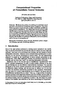
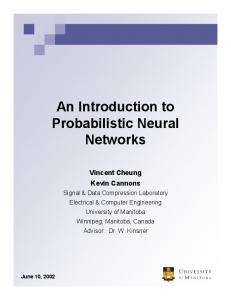
Note that jJX) is simply the sum of small multivariate gaussian distributions ten. tered at each training sample. However, the sum is not limited to being gaussian. It can, in fact, approximate any smooth density function. Figure 3.1 illustrates the effect of different values for the smoothing parameter o on ~JX) for the case in which the independent variable X is two-dimensional. The density

(a)

A small value of a

FIGURE 3.1 The smoothingeffect of different values of o on a PDF estimated from samples. [Ftvm Computer- On”ented Approaches ro Patrem Recognition (pp. 1(B101) by W. S. A4eisel, 1972, Orlando, FL: Academic Press. Copyright 1972 by Academic Press. Reprinted by permission.]

PROBABILISTIC NEURALNETWORKS

3.5

(b) A larger value of o

(c) An even larger value of a FIGURE 3.1 (Cont.)

‘s PIOttedfrom Eq (3 7) for three values of 6 with the same training samples in each case. A small value of G causes the estimated parent density function to have distinct “’odes corresponding to the locations of the training samples. A larger value of ~ pro‘Uces a greater degree of intewolation between points, as indicated in Fig. 3.1 b. Here, ‘a]ues of x that are close to the training samples are estimated to have about the same ‘rObabilitY of occurrence as the given samples. An even larger value of ~ produces a ‘rester degree of interpolation, as indicated in Fig. 3.1 c. A very large value of ~ would cause ‘he estimated density to be gaussian regardless of the true underlying distribution. ‘election of the proper mount of smoothing is discussed in Sec. 3.1.5.

3,6


Equation (3.7) can be used directly with the decision rule expressed in Eq (31), However, two limitations are inherent in the use of Eq. (3.7). First, the entire training set must be stored and used during testing; second, the amount of computation neces. sary to classify an unknown point is proportional to the size of the training set. When this approach was first proposed for pattern recognition [6, 101, both considerations severely limited the direct use of Eq. (3.7) in real-time or dedicated applications. Approximations had to be used instead. Computer memory has since become dense enough that storing the training set is no longer an impediment, but computation time with a serial computer is still a constraint. With large-scale neural networks with massively parallel computing capability on the horizon, the second impediment to the direct use of Eq. (3.7) is now being lifted.

3.1.3

Probabilistic Neural Network

There is a striking similarity between parallel analog networks that classify patterns using nonparametric estimators of a PDF and feedfowmd neural networks used with other training algorithms [1]. Figure 3.2 shows a neural network organization for classification of input patterns X into two categories. In Fig, 3.2, the input units are merely distribution units that SUPPIYthe same input values to all the pattern units. Each pattern unit (shown in more detail in Fig. 3.3) form a dot product of the pattern vector X with a weight vector Wi, Zj = X Wi, and then per. forms a nonlinear operation on Zi before outputting its activation level to the summation unit. Instead of the sigmoidal activation function commonly used for back propagation, ●

Y FIGURE 3.2 Organizationfor classificationof patterns into categories.

3.7


the nonlinear operation used here is exp [(Zi – 1)/~2]. Assuming that both X and Wi are normahzed to umt length, this is equivalent to using exp[ –(Wi – X)t(Wi - X)/2cr2] which is the same form as Eq. (3.7). Thus, the dot product, which is accomplished naturally in neural interconnections, is followed by the neuron activation function (the exponentiation). The summation units simply sum the inputs for the pattern units that correspond to the category from which the training patterns were selected. The output, or decision, units are two-input neurons, as shown in Fig. 3.4. These units produce binary outputs. They have only a single variable weight C (3.8)

wheren~ = number of training patterns from category A and nB= number of training patterns from category B. Note that C is the ratio of a priori probabilities divided by the ratio of samples and multiplied by the ratio of losses. In any problem in which the numbers of training samPles from categories A and B are obtained in proportion to their a priori probabilities, C = ‘t~tA. This final ratio can be determined not from the statistics of the training samPh but from the significance of the decision. If there is no particular reason for biasing the decision, C may simplify to –1 (an inverter). The network is trained by setting the w, weight vector in one of the pattern units ‘Clualto each of the X patterns in the training set and then connecting the pattern unit’s OutPUtto the appropriate summation unit. A separate neuron (pattern unit) is required for every training pattern.

fA(x)

fB(x)

Zi=XWi

u L 1

-1

z

gtzi)=exp ‘lGURE

3.3

A

0 1

[(Z,.1)102]

Patternunit (dot productform).

+ BinaryOutput

FIGURE 3.4

An output unit.


3.8

For a multiple category problem, the outputs of the summation units need to be multiplied by h~/@~ and then the output unit is replaced by a maximum detector.

3.1.4

Alternative

Pattern Units

Three alternative pattern units are shown in Figs. 3.5, 3.6, and 3.7. The pattern unit in Fig. 3.2 requires normalization of the input and exemplar vectors to unit length, but the pattern units of Figs, 3.5, 3.6, and 3.7 do not. The pattern unit of Fig. 3.2 can be made independent of the requirement of unit normalization by adding the lengths of both vectors as inputs to the pattern unit, as shown in Fig. 3.5. Figure 3.2 is a simplification of this, which shows congruence of the topology for PNN to that of BP. The pattern unit of Fig. 3.6 subtracts a stored exemplar vector from the input vector and sums the squares of the differences to find the euclidean distance (squared). This distance is input to an exponential activation function, which provides the response of one neuron to the summation unit. This version of the pattern unit is the most direct implementation of Eq. (3,7) and is often used. For basic PNN, the weights AJ and B shown in Fig. 3.2 all equal 1 and have no effect. It becomes necessary to have weights other than 1 when clustering is incorporated. The pattern unit of Fig. 3.7 performs the same function as that of Fig. 3.6, except that the “city block” distance metric is used instead of euclidean distance. We have noted in several practice problems that the two metrics work almost equally well. The city block metric is, of course, simpler to implement in parallel hardware, and was chosen for implementation in the DARPA/Nester/Intel chip available from the Nestor Corporation [11].

1

Zi=X”

Xi-~lXn2-~lXi12

2

t

g(Zi)=eXp[Zi/C2] FIGURE 3.5 A pattern unit. Dot product form k expanded to accommodatevectorsof any length.


x,

Xp

Xj

1

1

Ld -z

o

g(Z1)=eXp[- Zi/(2(J2] FIGURE 3.6 A pattern unit (euclidean distance form).

x,

Xp

Xj

j=l

,

t

t g(zi)=exp

[- Zi/Cf]

FIGURE 3.7 A pattern unit (“city block” distance form).

PRINCIPLES ANDALGORITHMS

3.10

The best pattern unit to use for a particular application will depend on hardware availability. Implementation technologies that lend themselves to vector subtraction will be best used with the distance-measuring forms, and those that lend themselves to vector multiplication [such as those using digital signal processing (DSP) chips, and optical computers] will be best used with the dot-product form. Fixed-point computa. tion is well suited for the distance-measuring forms, whereas floating-point computa. tion can be used equally well with either form.

3.1.5

Limiting Conditions as a + O and as a + ~

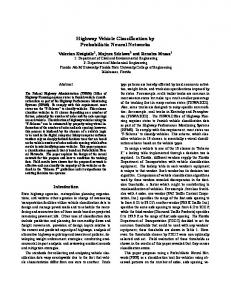
It has been shown [6] that the decision boundary defined by Eq. (3.2) varies continuously from a hyperplane when c + 00 to a very nonlinear boundary representing the nearest-neighbor classifier when o + O. The nearest-neighbor decision mle has been investigated in detail [12]. In general, neither limiting case provides optimal sepmation of the two distributions. A degree of averaging of nearest neighbors, dictated by the density of training samples, provides better generalization than basing the decision on a single nearest neighbor. The network proposed is similar in effect to the K-nearest neighbor classifier. Specht [13] contains an involved discussion of how one should choose a value of the smoothing parameter G as a function of the dimension of the problem P and the number of training patterns n. However, it has been found that in practical problems it is not difficult to find a good value of c, because the misclassification rate does not change dramatically with small changes in o. An experiment [10] in which electrocardiograms were classified as normal or abnormal according to the two-category classification of Eqs. (3. 1) and (3 .7) yielded accuracy curves that are typical for practical problems we have examined. In that experiment 249 patterns were available for training, and 63 independent cases were available for testing. Each pattern was described by a 46-dimensional pattern vector. Figure 3,8 shows the percentage of testing samples classified correctly versus the value of the smoothing parameter c. Several important conclusions are obvious. Peak diagnostic accuracy can be obtained with any o between 0.2 and 0.3; the peak of the curve is sufficiently broad that finding a good value of a experimentally is not difficult. Furthermore, any o in the range from 0.15 to 0.35 yields results only slightly poorer than those for the best value. It turned out that all values of G from O to - gave results that were significantly better than those of cardiologists on the same testing set.

I

95%

~

’90 -

3

Matchad-filter

8 Eao E E

-

Nemst-naighbor daciaiorlrule

I I 1 I I I I I I I 0 .05.10 .15.20 .25.30 .2.5.40 .45.50

70

I

I

I

I

.ao

.70

.ao

.90

. . . . . . . . . . . . . L. . . . . . . . . . . . . . 1.0

2.5

5

o

Smoothing Parafnatar,fJ

FIGURE 3.8 Percentageof testing samplesclassified correctlyversus smoothing parameter6.


3.11

The only parameter to be adjusted in basic PNN is the smoothing parameter cr, which is the same for every pattern unit and every dimension. In order for each input variable to have equal influence on the decisions of the netWork,it is necessary to prescale the input variables to have roughly the same range or standwd deviation. Standard deviations for each dimension should be computed by subtracting the category mean from each pattern vector and then pooling the data from all categories.

3,1.6 Associative Memory In the human thinking process, knowledge accumulated for one purpose is often used in different ways for different purposes. Similarly, in this situation, if the decision category were known but not all the input variables were known, then the known input variables could be impressed on the network for the correct category and the unknown input variable could be varied to maximize the output of the network. These values represent those most likely to be associated with the known inputs. If only one parameter were unknown, then the most probable value of that parameter could be found by ramping through all possible values of the parameter and choosing the one that maximized the PDF. lf several parameters are unknown, this method may be impractical. In this case, one might be satisfied with finding the closest mode of the PDF. This goal could be achieved by u5ing the method of steepest ascent. A more general approach to forming an associative memog is to avoid distinguishing between inputs and outputs. By concatenating the x vector and the output vector into one longer measurement vector X’, a single probabilistic network can be used to find Rx’), the global PDF. This PDF may have many modes clustered at v~lous locations in the measurement space, TO use this network as an associative memow, one impresses on the inputs of the network those parameters that are known, and one allows the other parameters to relax to whatever combination maximizes j7X’), which occurs at the nearest mode.

3“1”7 Speed Advantage Relative to Back Propagation APrincipal advantage of the PNN paradigm is that it is very much faster in training than ‘hewell-known BP paradigm ln the first practical problem in which the two paradigms ‘ere tfied on the same database (ship radar classification [14]), the time required for ‘NN was 0.7 s compared to over-the-weekend computation for BP. This result, a 200@00-to-1 improvement in speed is typical when the hold-one-out method of validation is used for both PlOJ and 13P When the available sample patterns are divided into ‘eparate training and test sets the s“peedup ratio ranges from 1 to 6 orders of magnitude [‘S1’ with sample sizes of u; to 10000 training patterns. The only exception to the ‘Expectationof large speed improvem~nts seems to be for overly defined problems, with ‘Uge redundant training sets.

3-1”8 Estimating a posteriori Probabilities ‘he ‘“tPuts ~JX) can also be used to estimate a posterior probabilities or for other purposes beYond the binary decision of the output units. The most important use we have found is to estimate the a postefiofi probability that X belongs to category k, F’[klXl. lf pattern x belongs to one and only one of c categories, then we have, from Bayes’ theorem,

3.12

PRINCIPLES ANDALGORITHMS

hkfk(x)

P[klX] =

~

(3.9)

hj~(X)

j=l

3.1.9

Probabilistic Neural Networks Using Alternative

Estimators of foo”

The earlier discussion dealt only with multivariate estimators that reduced to a dot prod. uct form. Further application of Cacoullos [9], theorem 4.1, to other univariate kernels suggested by Parzen [8] yields the following multivariate estimators (which are products of univariate kernels):

(3.10)

Ixj – Xkti]

lnp

dpi=~j=~ ?&

j,(x) = —

fk(x) =

Zll(

1-

when all lXj – X~ijl> p, the phenomenon of overi%ting is commonly ignored.

3.19

PROBABILISTIC NEUWL NETWORKS

Both Yand ~ can be vector variables instead of scalars. In this case, each component of vector Y would be estimated in the same way and from the same observations (X, Y), except that Y 1s now augmented by observations of each component. Note, from Eq. (3.20), that the denominator of the estimator and all the exponential terms remain unchanged for vector estimation.

3,3.3

Normalization of Input and Selection of Smoothing

Parameter Value

As a preprocessing step, it is usually necessary to scale all input variables such that they have approximately the same ranges or variances. The need for this stems from the fact that the underlying probability density function is to be estimated with a kernel that has the same width in each dimension. This step is not necessary in the limit as n ~00 and cr+O,but it is very helpful for finite data sets. Exact scaling is not necessary, so the scaling Variables need not be changed every time new data are added to the data set. After rough scaling, the width of the estimating kernel o must be selected. A useful method for selecting o is the holdout method. For a particular value of 6, this method consists of removing one sample at a time and constructing a network based on all the Othersamples. The network is then used to estimate Y for the removed sample. By repeatingthis process for each sample and storing each estimate, the mean-squared error can be measured between the actu~ sample values ~’ ~d the estimates. The value of O @ing the smallest error should be used in the final network. Typically, the curve of mean-squ~ed error versus ~ exhibits a wide range of values near the minimum, SOit iS not difficult to pick a good value for o without a large number of triah. Finally, the gaussian kernel used in Eq. (3. 1’7)could be replaced by any of the parzen windows.Again, the kernel of Eq. (3. 13) is attractive from the point of view of Computational simplicity. Using this kernel results in the estimator n

x ‘(x)=

Ci

Yi

exp

() –~

‘~,

exP (-:)

Ci = ~

Ixj – Xjl

(3.21)

where (3.22)

j=l

30304 clustering

and Adaptation

to

NonstationaW

Statistics

‘or ‘“me problems the number of observations (X, Y) maybe small enough that all the ‘ata obtainable CM’ be used directly in the estimator of (3.20) or (3.21). In other prob‘ems’‘he number of observations obt~ned may be large enough that it is no longer prac‘ical’0 assign a sep~ate node (or neuron) to each sample. Various clustering techniques can be used to group smples so that the group can be represented by only one node, ‘hich measures the distmce of input vectors from the cl~ster center. Burrasc~o [24] ‘as ‘Uggested using leming vector quantization to find representative samples to use ‘or ‘NN to reduce the size of the training set This same technique can be used fOr the Cunent Procedure Also ~-mems averaging ~25] adaptive K-means [26], one-pass~‘cans clustering “[271? or tie cluste~ng techniq~e used by Reilly et al. [281 for the

3.20


restricted Coulomb energy (RCE) network could be US~. However the cluster centen are determined, let us assign a new variable vi to indicate the number of samples fiat are represented by the ith cluster center. Equation (3.20) can then be rewritten as D;

m

E i=l

_—

“ “[l‘Xp

(262)

Y(x) =

D:

m

(3.23)

_— I j=l

“

Ai(k) = Ai(k – 1)+ P

‘Xp “[l

(202)

B(k) = B*(k – 1)+ 1

(3.24)

incremented each time a training observation Y“for cluster i is encountered; m < n is fie number of clusters. The method of clustering can be as simple as establishing a single radius of influence K Starting with the first sample point (X, Y), establish a cluster center X’ at X. All future samples for which the distance IX - Xil is less than the distance to any other cluster ten. ter and is also less than or equal to r would update Eqs. (3.24) for this cluster. A s~ple for which the distance to the nearest clusters is greater wan r would become the center for a new cluster. The numerator and denominator coefficients ~e completely determined in one pass through the datw no iteration is required to improve the coefficients. Since the A and B coefficients can be determined by using recursion equations, it is easy to add a forgetting function. This is desirable if the network is being used to model a system with changing characteristics. If Eqs. (3.24) are written in the form ‘r-l Ai(k) = —

A1(k–l)+:F

7:1

Bi(k) =—ll[(k [

T

Ai(k) = ~

{

Bi(k) =QBi(k–l) ‘r

new sample assigned to cluster i

-l)+: Ai(k – 1) I

I new sample assigned to a cluster # i (3.25)

then T can be considered the time constant of an exponential decay function (where Tis measured in update samples rather than in units of time). If all the coefficients were attenuated by the factor (t – 1)/r, the regression Eq. (3.23) would be unchanged; however, the new sample information will have an influence in the local area around its assigned cluster center. For practical considerations, there should be a lower threshold established for Z3i,so that when sufficient time has elapsed without update for a particular cluster, that cluster (and its associated Ai and Bi coefilcients) would be eliminated. In the case of dedicated neural network hardware, these elements could be reassigned to a new cluster. When the regression function of Eq. (3.23) is used to represent a system that has many modes of operation, it is undesirable to forget data associated with modes other than the cument one. To be selective about forgetting, one might assign a second radius p>> z In this case, Eqs. (3.25) would be applied only to cluster centers within a distance p of the new training sample. Higher moments can also be estimated with y’J substituted for y in Eq. (3.16). Therefore the variance of the estimate and the standard deviation can also be estimated directly from the training examples.


3.21

3.3.5 Comparison with Other Techniques Conventional nonlinem regression techniques involve either a priori specification of the fom of the regression equation, with subsequent statistical determination of some unde(e~ined constants, or statistical determination of the constants in a general regression equation, usually of polynomial form. The first technique requires that the form of the regression equation be known a priori or guessed. The advantages of that approach are that (1) it usually reduces the problem to an estimation of a small number of undeterminedconstants and (2) the values of these constants, when found, may provide some insightto the investigator. The disadvantage is that the regression is constrained to yield a “best fit” for the specified form of equation. If the specified form is a poor guess and not appropriate to the database to which it is applied, this constraint can be serious. Classical polynomial regression is usually limited to polynomials in one independent variableor low order, because high-order pol ynomials involving multiple variates often have too many free constants to be determined by using a fixed number n of observations (Xi, Yi). A classical polynomial regression surface may fit the n observed points Veryclosely, but unless n is much larger than the number of coefficients in the polynomial, there is no assurance that the error for a new point taken randomly from the distributionfix, y) will be small. Whh the regression defined by Eq. (3.20) or (3.21), however, it is possible to let o be small, which allows high-order curves if they are necessary to fit the data. Even in the limit as ~ approaches 0, Eq. (3.20) is well behaved. It estimates P(X) as being the same as the Y’associated with the Xi that is closest in euclidean distance to X (nearestneighborestimator)- For ~Y ~ >0, there is a smoo~ interpolation between the observed points (as distinct from the discontinuous change of Y from one value to another at Pointsequidistant from the observed points when 6 = O). Other methods used for estimating general regression Sufiaces include the back propagation (Bp) of errors neural network, radial-basis functions (RBFs) [29], the method of Moody and Dmken [261, CMAC [30], and the polynomial ratio approximation to Eq. (3.20) [31]. The principal advantages of GRNN me fast le~ing and convergence to the optimal ‘egression surface as the number of samples becomes very large. GRNN is particularly advantageous with sparse data in a real-time environment because the regression sur‘ace is instantly defined everywhere, even with just one sample. The one-sample esti‘ate is that ~ will be the same as the one observed value regardless of the input vector ‘o Asecond sample will divide hyperspace into high and low halves, with a smooth transition between them The surface becomes gradually more complex with the addition of each new sample point. The principal disadvmmge of tie technique of Eqo (3.20) is tie mount of COmpUtiltiOn ‘equiredof the trained system to estimate a new output vector. The version of Eqs. (3.23) ‘0(3”25)using clustering overcomes this problem to a large degree. Soon the development ‘f ‘eUral network semiconductor chips capable of performing all the indicated operations ‘nPmallel will greatly speed performance Almost all the neurons are pattern units and are ‘dentic~ The step and repeat microlitho&aphic techniques of semiconductor manufac ‘UnngW; ideally s~ite~ to replicating large numbers of identical cells. ‘inallY, GRNN can be combined with linear techniques. t When linear regression ‘x@ains mOst of the data in a database, a linear equation can be used for first-order estimation, leaving GRNN to model only the deviations from linear.

‘is ‘dea was pointed out by Dr Herbert Rauch, of Lockheed’s Pato Alto Research Laboratory.Fisher and ‘such [321have subsequently used &e GRNN combination with extended Katman filters for nonlinear control

Problems.

3.22

3.3.6

PRINCIPLES AND ALGORITHMS

Neural Network Implementation

of GRNN

Figure 3.9 is the overall block diagram of neural network topology implementing GRNN in its adaptive form, represented by Eq. (3.23). The input umts are merely dis. tribution units, which provide all the (scaled) measurement variables X to all the neurons on the second layer, the pattern units. It turns out that the first two layers, the input and pattern units, are identical to those for PNN. The pattern unit outputs are passed on to the summation units. The summation units perform a dot product between a weight vector and a vector composed of the activations from the pattern units. The summation unit that generates an estimate of flX)K sums the outputs of the pattern units weighted by the number of observations each cluster center represents. when Eq - (3.25) is used, this number is also weighted by the age of the obsewations. And K is a constant determined by the Pwen window used, but is not d~ta-dependent and does not need to be computed. The sum. mation unit that estimates YflX)K multiplies each value from a pattern unit by the sum of the samples P“ associated with cluster center Xi. The output unit merely divides ~flX)K by flX)K to yield the desired estimate of Y To estimate a vector Y, each component is estimated by using one extra summation unit, which uses as its multipliers sums of samples of that component of vector Y asso. ciated with each cluster center X’. There may be many pattern units (one for each exemplar or cluster center); however, the addition of one element in the output vector requires only one summation neuron and one output neuron. What is shown in Fig. 3.9 is a feedforward network that can be used to estimate vector Y from measurement vector X. Because they are not interactive, all the neurons can operate in parallel. Not shown in Fig. 3.9 is a microprocessor that assigns training patterns to cluster centers and updates coefficients Ai and Bi.

3.3.7

GRNN Examples

Estimators of the type described have many potential uses as models, inverse models, and controllers. Two examples are presented here. The first is a contrived example to illustrate the behavior of the estimated regression line. The second is an identification problem in controls first posed by Narendra and Parthasarathy [33]. A simple problem with one independent variable will A One-Dimensional Example. illustrate some of the differences between the techniques that have been discussed. Suppose that a regression technique is needed to model a “plant,” which happens to be an amplifier that saturates in both polarities and has an unknown offset. Its input-output (1/0) characteristic is shown in Fig. 3.10. With enough sample points, many techniques would model the plant well. However, in a large measurement space, any practical data set appears to be sparse. The following illustration shows how the methods work on this example with sparse data, namely, five samples at X = -2, – 1, 0, 1, and 2. When polynomial regression using polynomials of first, second, and fourth order was tried, the results were predictable. The polynomial curves are poor approximations to the plant except at the sample points. In contrast, Fig. 3.11 shows the input-output characteristic of this same plant as estimated by GRNN. Since GRNN always estimates using a (nonlinearly) weighted average of the given samples, the estimate is always within the observed range of the dependent variable. In the range from x = -4 to x = 4, the estimator takes on a family of curves depending on c. Any curve in the family is a reasonable approximation to the plant of Fig. 3.10. The curve corresponding to o = 0.5 is the best approximation. Larger values of 6 provide more smoothing, and lower values provide a

3.23


‘2

‘1

II

‘1

‘P

I

I Input Unft9

Pattern Unfts

2

Summation Units

ff(X)K

--- f(lQ K

--

$’ f(x) K \

7$

output

● 00

Units ? ;(x)

$lX)

FIGURE 3.9 GRNNblock diagram. clOseapproximation to the sample values phIS a “dwell” region at each sample point. ‘hen the holdout method was used, a = 0.3 was selected (based on only four s~ple P@mat a time). ‘e curve that would result from back propagation depends on a number of choices ‘aving to do with the configuration of hidden units, initial conditions, and other parameters.me main difference between Fig 3 11 and the cume resulting from radial-basis flln~tion~is that the ~BF ordinate would-decrease to zero for large values of lX1. Adqwive Contiol System.

The fields of nonlinear control systems and robotics are Panicultily good application ~eaS that can use tie potential speed of neur~ networks ‘m@ernentedin pma~le~hardw~e,

the adaptability of instant learning, ~d the flexibiltechnique cm be used. First, mode] the Plat as in Fig s ~* me “Gw~ ~ems tie relationships between the Inputvector (the input state of ~he sy~tem ~d tie contio~ ~~ab~es) ~d the simulated or actual output of the system ~onmol inputs cm be supplied by a nominal controller

ity

of a ~ompletel~ nonlinem formulation * sti~ghtfowmd

‘With‘andom variations added to explore inputs not allowed by the nominal Controller) ‘r by a ‘uman operator After the model is trained, it can be IMed tO determine control ‘nputsby an automated “what ir* svategy or by finding an inverse model. Modeling lnvO1vesdiscovering the association between inputs and OUtpUtS;SO~ inverse model


1.5 1.0 0.5 0.0 -0.5 -1.0,

-4 —

-3-

_2

“--l_

--”

o

1

2“

3

.4

Input FIGURE 3.10

Input-outputcharacteristicsof simple “plant.”

1.5 0.7 0.5

1.0

0.5

y

0.0

-0.5

-1.0

4

-3

-2

-1

0

1

2

3

4

x FIGURE 3.11 Input-output characteristics of plant of Fig. 3.10 as estimated by GRNN based on sample points at X = -2,-1,0, 1, and 2.

3.25


Control Inputs

T

b

Process, Plant, or System

WUtputs tate Vector

GRNN Model FIGURE 3.12

4

Modeling the system.

carIbe determined from the same database as the forward model by assigning the input variable(s) to the function of the desired output Y in Fig. 3.9, and the state vector and other measurements are considered components of the X vector in Fig. 3.9. One way the neural network could be used to control a plant is illustrated in Fig. 3.13. Adaptive inverse neural networks can be used for control purposes in either the feedforward path or the feedback path. Atkeson and Reinkensmeyer [34] used an adaptive inverse in the feedforward path with positional and velocity feedback to correct for residual error in the model. ~ey noted that the feedback had less effect as the inverse model improved from experience. They also used a content-addressable memory as the inverse model and reported good results. Interestingly, the success reported was based on using only single-nearest neighbors as estimators. Their paper mentions the possibility of extending the work to local averaging. Farrell et ~. [35] used both sigmoidal and gaussian processing units as neural network Controllersin a model reference adaptive con&ol system. They note that the gaUSSiaIlprocessing units have ~ advantage in con~ol systems, because the localized influence Of each gaussim node ~lows the le~ing system to refine its control fUIICt.iOtl h One EgiOn Ofmeasurement s.ace ~i~out degrading its approximation in dis~t regions. The Same advm~ge would hold true if Eq. (3.23) were used as an adaptive inverse. Naren&a and p~asuathY [33] separate the problem of control of nonlinear @unit systems into ~ identification of system (modeling) section and a model refer‘nce adaptive control (MRAC) section. Four different representations of the plant are ‘escribed. Output of the pkmt is (1) a linear combination of delayed outputs plus a non‘inear combination of delayed inputs; (2) a nonlinear combination of delayed outputs PIUSa linear combination of delayed inputs; (3) a nonlinear combination of outputs plus a ‘“nlinear combination of inputs; and (4) a nonlinear function of delayed outputs and ‘elayed inputs GRNN together with tapped delay lines for the outputs and inputs, cOulddirectly ~mpleme~t the identification task for the most general of these models ‘Which subsumes the others) This is true both for single-input, single-output (S1S0) “ants ad for multi-input, m&i-output (MIMO) plants. Once the plant has been identified (modeled) ~1 the methods of Ref 33 which are based on the back propagation ‘etWork [4]9 can’be used for adapting a “con’tioller to minimize the difference between

kir~

oltq)~ ~

GRNN Controller. —.

1

‘GURE 3.13

Control Inputs

m

Physical Plant

~t~ ~

*

!

A GRNN controller.

outputs . -

3.26


the output of the reference model and the output of the identification model of the plant This combination of technologies yields a controller with the simpler structure of BP but still uses the instant learning capability of GRNN for the plant modeling function. One of the more difficult examples given in Ref. 33 is example 4, for which & authors identified the plant using the type 4 model above. ln this example, the plant is assumed to be of the form yp(k + 1) =fip(k),

yp(k – 1), yp(k - 2), u(k), U(k – 1)]

(3.26)

where yP(k + 1) is the next time sample of the output of the plant, yP(k) is the current out. put, yP(k – 1) and y$k – 2) are delayed time samples of the output, u(k) is the current input, u(k – 1) is the previous input, and the unknown function ~has the form x,+ XJ X5(XJ- 1)+X4 m,? x,> x,, x., x,] =

(3.27)

1+X:+X;

In the identification model, a GRNN network was used to approximate the function ~ Figure 3.14 shows the outputs of the plant and the model when the identification proce. dure was carried out for 1000 time steps using a random input signal uniformly distributed in the interval [–1, 1] and o = 0.315. In Fig. 3.14, the. input to the plant and identified model is given by 2nk ‘ln 250

u(k) =

for k

500

{-

Figure 3.14 shows approximately the same amount of error between the model and the plant as does Ref. 33 (fig. 16); however, the GRNN model required only 1000 time steps

1

I

I

1

I

1

‘t—Httt—

-1

Hmim’i I

1 I

I

I

o

200

400

600

i

ti(l

3.14 Outputs of plant (dark line) and of the GRNN model (lighter line) after training with 1000 random patterns.

FIGURE

3.27

PROBABILISTIC NEURAL NETWORKS

to achieve this degree of accuracy,compared with 100,000 time steps required for the back propagation model used m Ref. 33. In other words, only 1 percent of the training was required to achieve compmable acc~acies. ne identification was accomplished with 1000 nodes in a five-dimensional space. No attempt was made to reduce the number of nodes through clustering. For back propagation, it maybe that for the 100,000 presentations of training points, the same 1000 patterns could have been repeated 100 times to achieve the same results. In this case, it could be said that GRNN learned in one pass through the data instead of 100passes. An experiment was performed to determine the extent to which performance degrades with fewer training data. The training set was reduced first to 100 patterns, then to 10 patterns. Figure 3.15 shows the output of the plant and the model when the identification procedure was carried out for only the first 10 random patterns of the 1000 (instead of the 100,000 used for IX’). The model predicted the plant output with approximately twice the error of the fully trained BP network, but using only 0.01 percent of the training data. Although it is not to be expected that equivalent performance would result from training with any 10 random patterns, this performance was achieved on the first trial of only 10 patterns.

3.3.8

Summary of Basic GRNN

The general regression neural network (GRNN) is similar in form to the probabilistic

neural network (PNN). Whereas PNN finds decision boundaries between categories of patterns, GRNN estimates values for continuous dependent variables. Both do so through the use of nonparametric estimators of probability density functions. The advantages of GRNN relative to other nonlinear regression techniques are as follows: 1- The network “learns” in one pass through the data and can generalize from exarnPles as soon as they are stored.

1

0.5

0

-0.5

-1

0

200

400

600

800

FIGURE 3.15 Outputs of plant(dark line) and of the GRNN model (lighter line) after training witJ only 10 random patterns.

3.28


2.

The estimate converges to the con&tiod mea rewession surfacesas more ad more examples are observed; yet, as indicated in the examples, it fo~s very rea. sonable regression surfaces based on only a few samples.

3.

The estimate is bounded by the minimum and maximum of the observations.

4.

The estimate cannot converge to poor solutions comesponding to 10C~ minima of the error criterion (as sometimes happens with iterative techniques).

5.

A software simulation is easy to write and use.

6.

The network can provide a mapping from one set of sample points to mother. If the mapping is one-to-one, an inverse mapping can easily be generated from the s~e sample points.

7.

The clustering version of GRNN, Eq. (3.23), limits the numbers of nodes and (optionally) provides a mechanism for forgetting old data.

The main disadvantage of GRNN (without clustering) relative to other techniques i5 that it requires substantial computation to evaluate new points. There are several waYs to overcome this disadvantage. One is to use the clustering versions of GRNN. Another is to take advantage of the inherent parallel structure of this network and design semiconductor chips to do the computation. The two approaches in combination prOvide high throughput and rapid adaptation.

3.4

ADAPTIVE

GRNN

Just as adapting a separate smoothing parameter for each measurement dimension ~eadsto greatly improved generalization accuracy for PNN, the same technique can be applied to the PDF estimation kernel for GRNN to greatly improve its accuracy. T’h.is ch~ge results in Adaptive GRNN. Like Adaptive PNN, Adaptive GRNN can be used for automatic feature selection. Again, the price paid for these benefits is the increased training time.

3.4.1

Adaptation

of Kernel Shapes

Adapting separate CT’Sfor separate dimensions is a bit simpler for Adaptive GRNN than for Adaptive PNN (Sec. 3.2.1) because the primary criterion to be minimized is inherently continuous. This criterion is the mean-squared error between the GRNN estimate (measured by the holdout method) and the desired response. Adaptation is accomplished by perturbing each 6 a small amount to find the derivativeof the optimization criterion. Then conjugate gradient descent is used to find iteratively the set of a’s that minimize the criterion. Brent’s method, modified to constrain the o’s to positive values, is used to find the minimum along each gradient line. After adaptation has progressed for several passes, some O’S will usually become so large that their corresponding inputs are almost irrelevant to the estimation of the dependent variables. These inputs are tentatively removed one at a time. If the resulting regression accuracy is improved or left the same, the input is left out.

3.4.2

Results Using Adaptive GRNN

Although basic GRNN has been found to be very valuable for interpolation and extrapolation of multivalued functions, the accuracy obtained with Adaptive GRNN is usuallY


3.29

b~tter~d often greatly improved. Table 3.2 shows comparative results for 13 databases of five distinct types. The pressure predictor k the prediction of pressure profiles in a rocket motor. Phase diversify refers to an optical wavefront sensor based on image data at two focal planes. The estimated wavefront can be used to correct for optical aberrations by controlling a deformable mirror. GRNN has been used to estimate the piston positions needed to bring the object into focus [36]. For the active sonar databases, GRNN was used to infer aspect angles of six different bodies. The accuracy criterion in Table 3.2 is the mean-squared error (A4SE) normalized by the variance of the predicted variable. Adaptive GRNN achieved significant reduction in the error rate in all cases. In addition, the numbers of features and of prototypes required were almost always reduced. Clustering, which was not used here, could further reduce the number of prototypes. Prototype pruning was not attempted on the pressure predictor database. An equivalent criterion, the multiple coefficient of determination R2, can be obtained by dividing the MSE shown by 10,000 and subtracting the result from 1.0. The improvement ratio, which is the ratio of the error rate for GRNN to that of Adaptive GRNN, varies from a minimum of 1.4:1 to better than 1-0:1 for these databases.

3,4.3

summary

of Adaptive GRNN

has shown that Adaptive GRNN usually greatly outperforms basic GRNN in terms of estimation accuracy. Adaptive GRNN differs from basic GRNN in that a separate smoothing paameter is adapted for each input feature. Adaptive GRNN also provides for automatic feature selection. Because large values of the smoothing p~ameter imply that the co~esponding input feature has little infhJence on the output estimateS, the algorithm tests for deletion of features. The reduction of the dimenslonalitY of feature space leads to increased generalization accuracy with finite training sets, h the experimental work repofled here, adaptation of the c vector was accomplished by using conjugate gradient descent. Other techniques for discovering the best combination of C’Sare possible. Ward Systems Group has recently used genetic algorithms for ‘his Purpose [23].

This section

3“5 HIGH-SPEED CLASSIFICATION ‘he ‘aJor disadvantage of PNN stems from the fact that it requires one node or neuron ‘or ‘ach training pattern Although training is extremely fast, classification of large ‘Umbers Of new pattems”can be S1OW because the amount of computation required tO classifYa new pattern is propo~ional to the number of neurons in the network. Special.puqose pwa~~e~hadwwe has ken developed to speed up classification. ‘ne ‘Xarnple is the DARpA/Nestorflntel Ni1000 chip, which has 512 parallel processors ‘hat perfom kernel compu~tions common to PNN, GRNN, RCE, P-RCE, ~d RBF ‘aradigms. Another is the Adaptive Solutions, Inc., CNAPS chip, which has a more gen‘ralSsingle-ins~ction multiple-data architecture. ‘n apProach to speeding up classification in a dedicated application is to simplify ‘he ‘etwork Several rese~chers have suggested various types of clustering techniques ‘0 ‘vercom~ the limitation These techniques yield a smaller number of cluster centers, ‘0 ‘hat each node represen~s a group of training patterns.

TABLE 3.2

Comparative Accuracy; MSE for Basic GRNN and Adaptive GRNN

Database

u &

Pressure predictor Stock forecast Sales forecast Sales forecast Phase diversity I Phase diversity 2 Phase diversity 3 Simulated active sonar Simulated active sonar Simulated active sonar Simulated active sonar Simulated active sonar Simulated active sonar

1 2 3 4 5 6

Original

Original

Basic GRNN

number of patterns

number of features

error rate (MSE X 10,000)

17,450 372 64 416 543 543 543 910 910 910 910 910 910

17 9 17 9 245 245 245 10 10 10 10 10 10

3 9,334 4,186 5,381 1,498 1,118 147 79 1,047 467 274 126 531

Adapted number of patterns 17,450 98 r 37 236 265 293 280 418 344 401 370 343 369

Adapted number of features

Adaptive error rate (MSE X 10,000)

Improvement ratio

8 6 8 9 39 43 50 8 8 9 8 5 10

2 6,936 1,117 1,410 349 225 56 14 277 119 72 12 64

1.5 1.4 3.8 3.8 4.3 5.0 2.6 5.6 3.8 3.9 3.8 10.5 8.3

PROBABILISTIC NEURALNETWORKS 3.5.I

3.31

Reducing NeWork Size by Using Clustering Techniques

[24] has advocated using Kohonen’s learning vector quantization (LVQ) technique to find representative exemplars to be used for PNN. Any standard clustering technique, such as K-mems clustering, can also be used for this purpose. Tseng [27] hasproposed using K-means clustering in conjunction with PNN in its dot product form. After expanding the dot product form (as in Fig. 3.5) to avoid the problem of unit normalization, he then used the K-means clustering algorithm with a lookahead feature to assign training patterns to particular clusters and to adapt the weights of the pattern units. In his formulation, patterns are assigned to the cluster which would be closest to the next pattern if the new pattern had been added to the cluster. Thus, pattern X~is assigned to clusterj which minimizes the quantity

Burrascano

(AJ+ 1)2 where AJ is the number of patterns represented by cluster j. As emphasized by Tseng [27], this technique provides a “conscience” which tends to add new patterns to clusters which have the smallest number of patterns. In his experiments, this look-ahead feature worked so well that a single pass through the data produced a condensed set which generalized nearly as well in classification of new points as basic pNN without clustering. For complex databases, multiple passes could be used to find the cOn&nsed set of exempl~s. The difference between the accuracy of basic PNN md clustered PNN could be used to determine when an additional pass is needed. To accommodate clustering, only the weighting function AJ, indicating the number of patternsrepresented by Clusterj, needs to be added to s~dmd pNN (Fig. 3.2). The weightingfunction modifies tie output of the associated pattern unit before it is added to the summationunit- The stored Coefflclents for cluster j ~e updated by the recursion equations

Aj(new)

= Aj + 1

The cluster centers me then used instead of individual training patterns in standard pNN. The s~e method of assigning patterns can be used with the distance-measuring pat‘em units of Figs. 3.6 and 3.7. Bezdek and Castelaz [37] have shown that fuzzy ~.means clustering is often, but IIOt “waYS,better than hard K-means clustering. ln fuzzy ~-means clustering, each new pat-

‘em’s assigned partially to all the clusters in proportion to its degree of membership to ‘ach cluSter as determined by a membership function. The membership function is a ‘eCreasing (unction of distance from the cluster center. The clustering technique of the ~e~tricted Coulomb energy (’CE) paradigm [28] can “so be used to find cluster centers and associated weights corresponding to the number ‘f ‘a~Ples represented by each cluster These can then be used with standard PNN as above. Nestor Corporation refers to thi~ combination as probabilistic RCE [111.

3“5’2 Reducing Network Size by Using a Mixture of Gaussian Techniques ‘raven [381 and Streit [39, 40] independently took approaches that use the concept of ‘Stimating probability density functions as mixtures of gaussian densities as pti of the

3.32


overall problem of classification or estimation. Traven estimates the pDF as a mixture of gaussian densities with varying covariance matrices, whereas Streit restricts the covariance matrices to being identical (homoscedastic) to fufier simplify the network and to use pooling of data to estimate the single covariance. Traven estimates a single PDF for all categories and estimates continuous variables instead of category classification. Both techniques can use far fewer gaussian nodes than training patterns. The following description is adapted from Streit and Luginbuhl [40]: Let p denote the dimension of input vector X, and let M denote the number of different class labels in the training set ~ of size Z For j = 1, . . . . M, let Gj 21 denote the total number of different components in the jth class mixture PDF. Let pti(X) denote the multivariate PDF of the ith component in the mixture for class ~, ~d let ~ti denote the proportion of component i in class j. The “within-class” mixing proportions ~ij me nonnegative and satisfy the equations Gj

Ij=]

nij = 1

The PDF of class j, denoted by f.(X), is approximated ed by gj(X), that is,

J.(x) =

gj(x)=

In Ref. 40, only multivariate Pti(X) has the form

J Zupti(x) i=l

homoscedastic

(3.28)

]=17...9M

by a gener~ mixture PDF, denot-

j=

1,,..,

M

(3.29)

gaussian mixtures are considered, hence

Pti(x) = (2Z)-P’21ZI-”2exp - *(X - ~~j)’z-’(x [

P’,j) 1

(3.30)

where pti is the mean vector, Z is the positive definite covariance matrix of PO(X),and superscript I denotes transpose. The covariance matrix Z is chosen independent of the class index j and the component index i. And IX denotes the determinant of matrix Z. Let h, denote the a priori probability of class 1.Let I!jldenote the loss associated with classifying an input vector X into class j when the correct decision should have been class 1. The risk pj(X) of classifying the input X into class j is the expected loss, so that (3.31) The decision risk pj(X) is thus approximated by a mixture of gaussian PDFs, as is seen by substituting Eq. (3.29) into Eq. (3.3 1). The minimum-risk decision rule is to classify X into that class j having minimum risk, that is, j = arg min {pj(X) ). The decision j is the optimum bayesian classification decision if gj(X) - J(X) for all j, that is, provided approximation (3.29) is an equality. The PDFs are estimated by a maximum likelihood method called the expectation-maximization (EM) method, which is described in Ref. 41. A brief description of the training algorithm for finding the mixtures of gaussian PDFs to be implemented in the nodes of PNN is given here. The mathematical justification is given by Streit and Luginbuhl [40]. The first step of the estimation process is somewhat arbitrag. It is necessary to specify in advance how many gaussian nodes will be assigned to each category and to give them starting centers and a common starting covariance matrix. The PDF of each cate-

3.33


~ou is estimated as the weighted sum of each of the gaussian densities (with the resrnc tion that the sum of the weights must equal 1, so that the integral of the sum over all measurement space is unity). Once the conditional PDFs are estimated, classification proceeds as in basic PNN. unlike hard clustering, each training sample for category j is considered to belong partially to every cluster node which comprises the estimate of the PDF for category j. Assignment of a sample X to each cluster i of category j is made in proportion to the likelihood PO(X) and is designated @u(X)” The sum of the proportions of sample X assigned to each component in its class must equal unity so that each training sample is assigned 100 percent to its category, although less than (or at most equal to) 100 percent to each component. Once this is done, the component means must be recomputed. The component mean ptiis the weighted average of all the training vectors in category j (weighted by Uu (X), the proportion of each sample in that component). The weight of the component m the estimation of the conditional PDF for category j is: T. +.+l)=l

J qk=,

(IJ :;)

I

(Xkj)

of s~ples with class label j. Next, the covariance is recomputed by using all the training samples from all the categories, but ~.. of the appropriate category j and component ~ is subtracted from each training vecto~ before being used in the computation:

where T-jis the number

The sumation portions

is over all

to be ass.gned

~~ning

to each

Categov

vectors j ~d

x

each multiplied by the computed proc$mponent i. Tis the total number Of train-

ing samples for all categories. The compu~tions indicated in tie last two paragraphs are repeated fOr n iterations ‘ntil a stopping criterion is satisfied. A typical stopping c~tenon is to stop when the likelihood function ~ as a function ‘f ‘teration number stops increasing at a sufficient rate. The likelihood function is the ‘urn of the log likelihoods for all patterns in the training sets,

‘ince ~ is positive definite matrix L-l Cm be chosen such that Z-l = (L-l)’L-’. If L-* is chosen to be the Cholesky ~actor of X-l, then L-l is lower triangular. The Cholesky fac‘or (sometimes referred to as the “squ~e root” of the matrix) can be computed easily by ‘sing tie algorithm in Ref .,42 section 29. . Substituting into Eq. (3.30) yields

1 _ +x -L,-lp,lz =(2z)-NIZl-in (

PU(X) = (2n)-PnlH-112 exp - ; (X - pJ(L-’)’L-’(X [ exp

‘here ~“~is the usual euclidean norm on RN-

z

lJ

- Pti)

(3.32)

)

3.34


Alternatively, matrix L can be chosen so that it characterizes the discrete KmhunenLoeve transformation corresponding to Z, that is, L-l = A-In V, where Z = UA@ However, the Cholesky decomposition requires less computation to determine L-l ~d less computation in the evaluation of Eq. (3.3 1), since L.-l is then lower triangular. A neural network topology for implementation of classification using the mixtureof-gaussians technique is shown in Fig. 3.16. It is similar to, but more general than, tie PNN topology of Fig. 3.2. Between the input units and the pattern units are now placed p L-l transform units, which perform the function of rotating the measurement space to

xl

x

1

(3

Xp

1

●

●

0

(n

1

$

99*

●

Input Units

0

Risk Units

t P1 (x)

FIGURE 3.16 Luginbuhl).

+ Pj(x)

t

PM(X)

Probabilistic neurat network using mixture of gaussian densities (after Streit and

3.35


a new set of axes. The gaussian mixture components are identical to the pattern units, except for the method used for training and the n coefficients, which give the components weight in proportion to the number of training samples represented. The summation units are unchanged. The risk units implement the minimum risk strategy for decision making for multiple categories, and are equally appropriate for basic PNN with multiple categories. As pointed out to me by Dr. Roy Streit [43], estimation of PDFs by a mixture of gaussian densities can proceed iteratively in the same way with or without constraints on covariance matrices. If the covariance matrices for all nodes are constrained to be the same and diagonal, the procedure will simultaneously find a set of prototype vectors and the set of variances. When this is done, the L-l transform units of Fig. 3.16 can be eliminated if the input units perform a simple division of the raw input by the square root of the corresponding variance term. From this diagram, it is clear that the benefit of restricting mixtures to homoscedastic kernels is that only one L.-l transform has to be performed on each input (pattern) vector.After that, the pattern units, of which there may be large numbers, can be as simple as those described in Fig. 3.6. Since the pattern units of Fig. 3.5 are mathematically equivalent to those of Fig. 3.6, the entire network, with the exception of the exponential activation, can be implemented by using multiply/accumulate chips common for digital signal processing. Note that the Adaptive PNN of Sec. 3.2 can be used very effectively to reduce the dirnension~itY p of the patterns before any of the clustering techniques are applied.

3.6 ONE CATEGORY AND PROVISION MIKNOW/V CATEGORIES

3$.1

FOR

Detection

Men it is necessary to classify a pattern as the category of interest versus everything “se) it maybe impractical to get a sufficient number of training samples for “everything ‘]Se.” In this case it is important to train a PDF on just one category and then establish a threshold on th~t PDF.

ln most of the classification problems discussed, the kernel parameters were determined based on classification accuracy. The PDFs for one category by itself can be esti‘ated by using maximum likelihood to establish the values of the smoothing parameters ‘0 be used Refernng back to @ (3 7) which is the likelihood of pattern X belonging ‘0 catego~ k, we see that the likelihoo~ (Ml) that all patterns X~ibelong to category k ‘s ‘he sum of the logs of ~~(X) evaluated at each pattern (using the holdout method to avoid an artifici~ maimum at G = 0).

~xti-xkjp Log LH = ~ log,~l jsl”

~2Z)fi,,UP exp(-

2cJ2

)

j*i

‘he best * for tie One-categog case cm be found as ~~ value that ‘“g

likelihood. ‘he log likelihood

cm

~so

be mmifized

with

more

th~

one

free

maximizes

the

p~ameter such as

a ‘epUate smoothing parameter for each dimension or the m.ixture-of-gaussians dure of the previouS section.

proce-

3.36

PRINCIPLES AND ALGOFUTHMS

In any of these cases, the threshold on the estimated PDF will have to be dete~ned on the basis of the number of false-positive detections or musses one IS able to tolerate,

3.6.2

Different Kernels for Different Categories

In many problems, it is clear that the underlying probability distributions are quite different for different categories. Again, the maximum-likelihood technique can be Used separately for each category (with or without the rnixture-of-gaussians technique of &~. 3.5). It is also possible to optimize classification accuracy by adapting separate C’S for each category. The choice between selection of o based on classification accuracy or selection based on maximum likelihood depends on the problem to be solved. Selection based on classification accuracy optimizes the value of a at the decision boundv, with little coucem for estimating the shape of the PDF in other regions. On the other hand, estimation based on maximum likelihood is better when categories have widely differing vti~ces, and therefore one size-estimating kernel is not appropriate for all categories.

3.6.3

Unknown Categories

Most neural network classifiers are based on the assumption that all patterns belong to one of a fixed set of possible categories. When examples of a new category, for which there have been no training examples, first appear, it is impotit not to classify them into one of the known categories. instead, the classifier should recognize novelty in the new patterns and establish a new category. This can be accomplished within the framework of PNN by simply postulating an unknown categoxy (lUand then assigning lower values of loss to misclassification of a pattern from a known category as unknown than the loss associated with misclassifying the pattern into the wrong known category. To simplify the following ~~ysis, (i is defined as the loss associated with misclassification of a category i pattern as belonging to any other known category. In addition to supplying values for the {i’s, the user must supply rough approximations for the following values: ●

/d, the loss associated with misclassification into a known category

of a pattern from an unknown category

●

(~U,the loss associated with misclassification categories as an unknown

of a pattern from any of the Zt’known

●

hi, the a priori probability of observing a pattern from category i

●

hU,the a priori probability of observing a pattern from a new category (unknown)

●

~u(x), tie pDF for unknowns ~d assumed uniform over the range of measurement variables

The loss values {i are always larger than {b. ~~ mayor may not be equal to ~uE The risk associated with classifying a pattern X into one of the N known categories e: is then J

Risk (0= ej) = t’#u~U(X) + ~ #~i~(X) icl i*j

T’he risk associated with classifying a pattern X into the unknown category is

3.37


The decision to classify the pattern X into one of the N known categories is

d(e=ej)

ifejhjjyx)>e,hi~(x)

foralli#j

and

l?uklzufu(x) +f t?,hi&(x) < tku ‘f hij(x) i=~ [.71 i*j

The decision to classify the pattern X as an unknown is made if the second condition is not true. These decision rules replace the original PNN decision rule of Eq. (3.4). An example of this approach, using multispectral imagery, involved the classification of clouds agtinst a background of ice and snow. Meteorologists and photo interpreters have traditionally

done poorly

with this problem,

since everything

looks white.

A 12-channel imager produced the image in the California Sierras near the town Of Bndgepofi shown in Fig. 3.17. ~i~y-seven pixel samples each were collected of clouds, snow, water, bare soil, and runoff. These were used m training examples for their respective Categories. me classified image (Fig. 3. 18) shows tie results with clouds labeled w~te, snow, water, b~e soil, and runoff labeled by V~OU,S shades of gray as shown, and unknown labeled black. In this case, unknown tends to indicate only transition Pixels on the border between one category and the next. What seemed to impress the meteorologists tie most was the Co=ect classification of snow and water in shadow regions produced by the clouds. The Pm used only tie pixel vectors for classification wi~ no other contextual hforrnation. This s~e neural network was given a new image to classify, taken over Mono Lake. ‘e known categories all appear to be correct, and three significant regions of unknown Pixels are obvious in tie classified image (Fig. 3.19). These regions area region of lava>

FIGURE 3.17

Natural color image.

c1Clouds c1,,

Water

$$ D

Runoff

E

Snow

Bare soil Unknown

an island covered with seagull droppings, and Highway 395 (asphalt). These were correctly identified as unknown because no examples of these regions were provided in the training. We now have the option of adding the pixels from the lava, island, and highway to the PNN as new categories or as additional samples of the old categories (for instance, lava may be chosen to be another example of bare soil).

3.7

RADIAL-BASIS

FUNCTIONS

Neural networks based on localized basis functions and iterative function approximation are usually referred to as radial-basisfinctkm (RBF) networks. RBF networks have a long history, dating back to the Russian school of Bashkirov et al. [44] and Aizerrnan et al. [45], at which time the networks were referred to as the method of potential @nctions, They were introduced with the more descriptive name by Broomhead and Lowe [29], Moody and Darken [26], and Poggio and Girosi [46]. Classification of new patterns is done in much the same way with RBFs as with PNNs. In both cases, localized basis functions respond strongly when the input vector presented is similar to the center of the basis function. The response of the localized basis function falls off rapidly as the distance between the center of the basis function and the input vector gets large. In the simplest case, the output of the network is a linear combination of all the basis function responses (see Fig. 3.20). Again, the pattern

PROBABILIS~C

NEURAL NETWORKS

FIGURE 3.19 MonoLake image with PNN classifications.

Units can be ~ep~e~e~te-j

by

Fig.

3,6, 3.7, or 3.5. The oUtput unit multiplies each pattern

Unitactivation by a weight, sums them, and adds a bias. ‘he most significant difference between RBF and PNN is the method of trtining. Training tie RBF consists of iterative~Y adapting ~~e parameters Oftie network Until the Outputapproaches the desired output over the whole r~ge of Kaining patterns. The ~F network is inherently a regressionnetwork and so estimatesthe value of a COIlhIlllOus Variable when it is desired to use tie RBF as a two.categov classifier, the desired OUtPlltis u&ally set to +] for one ~ategow ad _l for the other. The parameters Of the network ~hlch can be adjusted me not only the output weights W but also tie centerS Of the basis functions and my or all of their shape parameters. There me as many Vtiations and nuaces to ~Fs as here are to pNN and GRNN ‘et~orks. Although space does not permit going into all of them here, ~will m~e ‘ome lleneral comptisons. 1“ ‘BFs always cluster whereas pms have to have clustering added.

are

defined

with one node per training point and

2“ ‘n RBF network Cm be assigned a fixed number of nodes. The complexity of the ‘etwork does not grow as new training samples become available. 3“ ‘e fixed number of nodes can be small, leading to efficient classification mation from new I)atterns. 4“ It’s easy to mix n~des of different widths and other parameters.

or esti-

PIUNCIPLES AND ALGORITHMS

3.40

xl

Xj

Xp

Input Units

Pattern

Units

output Unit

Y

A w

FIGURE 3.20 A radial-basisfunctionnetwork.

On the other hand, PNN and GRNN have certain advantages based on their roots in probability theory: 1.

PN_Ncan begin to classify after having just one training pattern from each category; GRNN can begin to estimate after having just one training pattern.

2.

In addition to classifying patterns, PNN is able to estimate the probability that a pattern belongs to a certain class.

3.

Novelty detection is possible, and the method for classification into the “unknown” category is easily justified.

4.

The principal of maximum likelihood can be used to estimate the parameters of the kernel.

5.

For small training sets, PNN and GRNN train instantaneously and can begin classification in real time. When the training sets are large enough that clustering is required, this advantage disappears.

PROBABILISTIC NEW

NETWORKS

3.41

6, Detection is possible by estimating only a single PDF and thresholding. 7. It is easier for the humm to understid why it is not working when it is not.

how the network works, or to understand

one variant of RBF which has interesting qualities is the resource allocation network of platt [47]. It does not start out with a fixed number of nodes; it allocates just enough nodes of varying widths to obtain the desired accuracy on the training set. This results in a very fast network for production estimation problems. In our laboratory we have alsomodified it to be a classifier by adjusting the targets to be + 1 or -1. In training, there is no error correction if the network produces a value > +1 for a desired+ 1, or for a value J R~ya/ Stutis~ical Society, series B, VOL39, pp. 1-38, 1977.

‘.’.

‘. ‘. ~ess B p ~’m.e~, s A Te~olsky, and W. T. Vetterling, Numerical Recipes in ‘onran: ~1 A; ofscientific Computing, 2d ~., Cambridge University Press, New York, 1992. ‘“y ‘~eit, Personal co~unication ‘%st 7-11, 1990.

at Naval Underwater

Systems Center, Newport, W,

3,44

PRINCIPLESAND ALGORITHMS

44. 0. A. Bashkirov, E. M. Braverman, and I. B. Muchnik, “Potential Function Algorithms for Pattern Recognition Learning Machines,” Automation and Remote Control, vol. 25, ~P, 692-695, 1964. 45. M. A. Aizerman, E. M. Braverman, and L. I. Rozonoer, “Theoretical Foundations of potential Function Method in Pattern Recognition,” Automation and Remote Control , VO1.25, Pp. 917-936, 1964. 46. T. Poggio and F. Girosi, ‘6ATheory of Networks for Approximation and Learning,” A.I. Memo 1140, Artificial Intelligence Laboratory, Massachusetts Institute of Technology, Cmbridge, MA, July 1989. 47. J. Plan, “A Resource-Allocating VO].3, pp. 213-225, 1991.

Network for Function Interpolation,”

Neural Computation,

PNN: FROhf

FAST TRAINING Donald

Lockheed

Mafiin

F.

TO FAST RUNNING

Specht

Missiles

&

Space

Palo Alto Research Laboratories Palo Alto, California 94304 USA email: specht@pc-smtp. rdd,lmsc,lockheed.

com

INTRODUCTION The Probabilistic Neural Network (PNN) is no longer a single paradigm, but has blossomed into a family of paradigms which are suited to different types of problems from database exploration to production systems, While all are rooted in statistics (hence the name), there is heavy reliance on iterative algorithms typical of neural nets. Basic PNN describes a parallel architecture to make Bayesian decisions based on a nonparametric estimation of probability density finctions. Adaptive PNN involves iterative optimization of the parameters of the Parzen window. The process of optimizing the parameters can also be used for feature selection. After features have been selected and adequate classification accuracy has been demonstrated, it is important to reduce the size of the network so that the computation required for classification of new vectors in production is minimized. It will be shown that Maxirnurn Likelihood Training of the PNN [ 1] (MLT-PNN) yields small, fast runtime modules which can be programmed into efllcient code or built into hyperfast hardware. In the past it has been advantageous to explore new databases and features using basic PNN because of its fast training speed, but that left a requirement to do something different to speed up the resulting runtime system. MLT-PNN provides a means for finding runtime modules which are just as eilicient as multi-layer perceptions, but do not require the designer to abandon the statistics-based approach. The third leg of the system is Adaptive PNN which can accomplish feature selection because its optimization criterion is classification accuracy, whereas MLT-PNN optimizes representation of PDF’s in a fixed dimensional space. A similar progression of techniques estimation of continuoLls variables.

applies

to General

Regression

Neural

Networks

(GRNN) for

BASIC PNN The most basic form of the Probabilistic Neural Network consists of a parallel network of processing elements (or neurons) which implement the estimation of probability density fhnctions (PDF) for each category (using Parzen window approximations), and which classi~ new patterns Input patterns X consist of a set of p measurements which, after using the Bayes strategy. scaling, are applied to a number of paftert~ Imifs. The output of each pattern unit is impressed on the sun~n~a(io)~ u)jif corresponding to the classification of the corresponding pattern. Each summation unit generates the a posteriori probability p[class j I X]. The classification output is’ determined by the 0UIP141utlif which finds the j which maximizes the fhnction p[class j I X] times p(j] times the loss associated with misclassification ofa classj pattern. The pattern units measure the distance between the input pattern X and the pattern stored in that unit, and then form an output based on the distance using a nonlinear actii’atio)~fi)lctio)l. When the distance measure is Euclidean and the activation fimction is exponential, then the Parzen window is Gaussian with parameter a. The G can also be considered the smoothing parameter of the estimated PDF. A fill description of basic PNN with its variations is presented in references [2,3] and will not be repeated here, “Training” of the network consists of storing one training pattern in each pattern unit and then adjusting the one free parameter, a, for maximum accuracy on a test set. Training of basic PNN is thus extremely fast since only a few values of a need to be tried to find one which is close to maximum accuracy. On the negative side however is the fact that one neuron must be dedicated to each and every training pattern. This problem is usually overcome by using some form of clustering [4] and then dedicating one pattern unit to each cluster center instead of one to each” raw pattern. There are four variations for implementation of the pattern units in the PNN network[4]. In two variations (the dot-product forms), the topo!ogy of the PNN is similar in structure to the multiIayer perception (MLP), differing primarily in that the sigmoid activation fi.mction is replaced by an exponential activation finction, and that the training is entirely different.

ADAPTIVE

PNN

Up to this point, the description of PNN has been limited to discussion of a single smoothing parameter which is applied in the same way to all measurement variables; that is, the PDF estimation kernel has been radially symmetric. The only special treatment for individual measurements is the scaling of input measurements to be all in the same range (usually by dividing by the standard deviation of each measurement).

z

An important improvement to PNN, called Adaptive PNN, is obtained by adapting separate smoothing parameters for each measurement dimension. This oflen greatly improves the generalization accuracy. The dimensionalit y of the problem and the complexity of the network can usually be simultaneously reduced. Adaptive PNN can be used for automatic feature selection. The price paid for these improvements is increased training time.

Adaptation

of Kernel Shapes

Basic PNN estimates PDFs as the sum of Gaussian kernels which all have the simple covariance matrix, a21, where I isthe identity matrix. PDFs can also be estimated as the sums of Gaussians with a fill covariance matrix. However, the complexity of a till covariance matrix may not be justified for many problems. Also, the use of a fill covariance matrix does not lend itself to automatic feature selection as does the method to be described. We have found that the simpler technique of adapting separate o’s for each dimension greatly improves generalization accuracy. Two adaptation methods have been used. The first, described in Ref. [4], uses gradient descent with two optimization criteria. The controlling criterion was classification accuracy, using the holdout method for validation. Whenever the change to the o vector was too small to cause a change in classification accuracy, the sum of probabilities, which renders a continuous criterion, was computed, The sum of probabilities is defined as the sum over all patterns of the probability that the pattern is correctly classified (using Bayes theorem). In the second method [5], adaptation is accomplished by perturbing each a a small amount to find the derivative of the optimization criterion with respect to each sigma. Then conjugate gradient descent [6] (ascent) was used to find iteratively the set of a’s that maximize the optimization criterion. Brent’s method [6, Chapter 10], used for finding a maximum along a gradient line, was modified to constrain the G’S to positive values. The second optimization criterion emphasizes improvements in catego~ separation only between categories where misclassifications occurred. When patterns horn catego~ k are misclassified as members of category q, the likelihood ratios, LR = fl@)/fq(X), are calculated for all category k patterns, using the hold-one-out validation method. The hold-one-out validation method consists of computing fk(X) except that the pattern unit storing X = Xki is not used in the summation when evaluating pattern i. The mean log likelihood ratios of misclassified and correctly classified patterns are calculated separately, and their ratio is taken. This ratio is summed over all cross categories where misclassifications have occurred. The following criterion is then maximized:

xx

A4ea]l log LR for

, ,*, A4eatt iog LR for

mischssijed

correctly

patterns

classl~ed

(CAT, I CA T )

patlerns(CA

T, I CA Tq)

This criterion also provides a continuous measurement of .c!assification improvements smaller than integer classification counts can be detected.

accuracy

so that

3

This adaptation, with a criterion of separating classes rather than simply estimating PDFs, not only finds a separate smoothing parameter, a, for each variable, but also identifies variables that are poorly correlated with the desired output, It will be noted that variables with a large o have a relatively small effect on the estimation of PDFs. After adaptation, as described above, has progressed for several passes, resulting in some variables being almost irrelevant to the classification decisions, these variables are removed one at a time and are left out if the resulting classification accuracy is improved or the same. Thus, adaptation of O’S can also be used for feature selection and dimensionality reduction.

Results Using Adaptive PNN Nine databases had been tested using the original version of Adaptive PNN. Six additional databases were tested using the new version, The results are shown in Table 1 below. All of the databases represent real problems with overlapping distributions and measurements contaminated with noise. Databases A through E and J through O came fi-om sensor measurements with naturally occurring noises; simulated noise was used for F through I. Table 1. Comparative accuracv.

accuracy: adapted smoothing parameters per feature versus standard PNN

Database A Drawings of3-D parts B Aircrafi health monitoring C Automatic targeting D Automatic targeting E 97 categories F 17 cats active sonar G Missile track discrimination H Missile track discrimination I Missile track discrimination J Multispectral imagery K Voice grade L Thematic mapper sensor M Hyperspectral Aviris imagery N Engine misfire detection 0 Propellant pressure

Number of Patterns

Original Number of Features

73 90 270

21 16 9 9 3 9

792 4187 1530 498 1684 3570 756 3037 628 648 2520 58

10 10 10

12 10

12 209 4 51

Basic Pm Accuracy (%)

Adapted Number of Features

74 78 93 94 72 95 92 97 97 98.68 97.05 92.25 94.33 77.54 97.3

5 6 4 5 3 7 3 2 4 6 8 6 122 3 21

Accuracy with Adapted ~ 93 95 97 98 74 95 95 100 99.4 100 99.44 96.26 100 37.40 100

Adapting just the p smoothing parameters (one for each measurement) does not increase the complexity of the trained network, because the usual preprocessing needed for PNN requires division of each variable by its standard deviation or range to ensure that the numerical ranges of all input variables are comparable. Since the smoothing parameters are used subsequently but in the same way, they can be combined with the preprocessing divisors.

The Adaptive PNN described here, while ofien finding a reduced feature set and greatly increased accuracy, is iterative and trains more slowly that basic PNN. The advantages of Adaptive PNN depend on the underlying distributions in the database. For Database E, for example, no dimensionality reduction was possible and the adapted a’s were almost equal; in this one case, the advantage of Adaptive PNN was insignificant.

PEAK OF ACCURACY SURFACE EASY TO FIND IN SIGMA SPACE What is the best method for searching the range of possible smoothing parameters to find the best set of a’s? In the last section two different methods were tried and both produced extremely good results. But, in fact, neither technique is optimized. The fact is that the accuracy surface in a space defined by the a parameters is much easier to search than the accuracy surface defined by the weights in a multilayer perception, for example. One reason is that there are only p free variables in Adaptive PNN (where p is the number of input variables) whereas there are many more free variables in an MLP. Another is that there is only one level of weights in Adaptive PNN rather than the complex interaction in the MI-P. In some problems, almost any (s vector is a satisfactory solution. An example of this is plotted in Figure 1, where classification accuracy is plotted as a fimction of two of the 10 O’S. This plot represents real data from a voicegrade receiver classification problem. As can be seen from the plot, almost any combination of o’s yields a classification accuracy of about 98’Yo.

100

1

Sigma - Feature 1

Sigma - Feature 2

Figure 1. Classification accuracy as a function of two of the 10 smoothing parameters.

hotherillustration of theease ofselecting smoothing p~meters isshownin Figure2. Figure2, representing the separation of two normal distributions in one dimension (with means of 2 and 5 and SD= 1) shows in part (a) that the plot of accuracy versus ts has a wide peak which should be easy to find in a short exploration of values for O. Figure 2b, on the other hand shows accuracy as a flmction of weights on a single layer pert.eptron. Even a single layer perception has two weights, the input weight and a bias weight, and so the one dimensional search has been replaced by a 2 dimensional search. As can be seen in Figure 2b, many values of the weight vector correspond to poor accuracy, whereas any random value of o in Figure 2a yields reasonable generalization accuracy. ~m. w m. z

(a)

P“’ 2 80. 50. u“ o

02

04

06

01

1

%7-

(b)

-+

/

5

0 -5 WI

-lo

-.10

Wo

Figure 2. a) Classification accuracy as a function ofa for a PNN classifier. b) Classification accuracy as a function of the weights of a single layer perception using the same data. The artificial data was designed so that the optimal decision boundnry could be achieved by a single Inyer (linear) perception. Figure 1 shows, curiously enough, that a slight improvement in accuracy can be achieved by allowing the G of the Iefl axis to grow without bound. In this case, the slight improvement in accuracy is not of significance, but the demonstration that making the corresponding measurement and all the related calculations unnecessary is important.

Figure 3 shows a similar classification accuracy surface which indicates that one of the two measurements is not only unnecessary but has indefinitely responsible fordegrading the accuracy of the network, A good search routine would easily find that high values for o on the right axis Adaptive PNN would test to see if complete would improve the accuracy of the system. The data shown is two of the 21 elimination of the corresponding input was possible. measurements for Database ~ Table 1. One of the measurements was one of the 5 that remained after the Adaptive PNN run, and the other was one of the 16 that were removed.

100 1

Sigma - Feature 1

Sigma - Feature 2

Figure 3. Classification accuracy as a function of two smoothing parameters. is real data from Database A, Table 1.

Data shown

If a gradient search technique is to be used, the discrete nature of figure 3 leads to many areas of zero gradient. To avoid that problem, the criterion to be maximized in Adaptive PNN was set to be the sum of the probabilities of correct classification summed over all the training patterns using the hold-one-out evaluation technique. This does provide a smooth surface, as shown in Figure 4, which can be searched using gradient techniques.

7

Sigma - Feature 1

Sigma - Feature 2

Figure 4. Sum of probabilities from Database A, Table 1.

as a function of two smoothing parameters.

Data shown is

Since the accuracy surface to be searched for a good o vector is so uncomplicated, many techniques could be adopted. Ward Systems Group has implemented a genetic algorithm for this purpose, and with good success[7]. HIGH-SPEED

CLASSIFICATION

In the past, the major disadvantage of PNN has been that it requires one node or neuron for each training pattern. Although training is extremely fast, classification of large numbers of new patterns can be slow because the amount of computation required to classifi a new pattern is proportional to the number of neurons in the network. Special-purpose parallel hardware has been developed to speed up classification. One example is the DARPA/Nester/Intel Ni 1000 chip[8], which has 512 parallel processors which perform kernel computations common to PNN, GRNN, RCE, P-RCE, and RBF paradigms. Because it was designed specifically for kernel computations, tradeoffs had to be made between dimensionality, number of nodes, weight resolution, and number of decisions per second. There is a need for a family of these chips with different tradeoffs for different classes of problems. Another chip

solution is the Adaptive Solutions, Inc., CNAPS chip, which is a more general, single-instruction multiple-data

architecture.

up classification in a dedicated application is to simplifi the network. Several researchers have suggested various types of clustering techniques [9,10] to overcome the limitation. These techniques yield a smaller number of c!uster centers, so that each node represents a group of training patterns. An approach

to speeding

In addition to standard clustering techniques cluster boundaries, there are sofi clustering (overlapping) clusters.

in which the clusters are characterized by hard techniques which result in a fewer number of

SOFT CLUSTERING Compact data sets for training can be obtained by clustering and using the cluster centers as nodes for PNN. Even more compact data sets can usually be obtained by using overlapping clusters (soft clusters rather than hard-bounded clusters). A technique developed by Streit and Luginbuhl [1, 11] uses the principle of maximum likelihood to estimate PDF’s as a mixture of Gaussians. They recommend forcing all of the components to have the same covariance matrix (distributions which have the same covariance matrix are said to be homoscedastic). This has two advantages: A) The resulting PNN can be implemented by means ofa single linear transformation (rotation) of the input vector followed by the normal PNN structure. B) Pooling of data from all of the components of all of the categories is used to estimate the single covariance matrix. If this were not done, it would be far more likely that some of the components or categories would represent so few training samples that the resulting covariance matrix would be ill-conditioned. The following is an overview of the method used. For a more-complete description, including the equations for calculating the parameters of the network the reader is referred to [1] or [12].

Overview of the method: 1) 2) 3) 4)

Class PDFs are estimated as sums of overlapping Gaussian components. Each Gaussian component has a different weight and mean, but the same covariance matrix. Each training sample has a weighted membership in each Gaussian within the class. Initialization: Choose number of components for each class. Assign a mean vector to represent each component (initial values are not critical). 5) Iteration: a) The weight of each training sample X for each Gaussian component within the class is established as the likelihood of X for that Gaussian component normalized by the sum of the likelihoods for all components. The sum of the weights for sample X in all components = 1. The weight of the sample for all components of other classes is zero.

b) Afier the weights have been established as above, the weighed average of all the patterns for each component becomes the mean vector of that component. c) Similarly, the weight of the component is the sum of the weights of all the patterns. d) Similarly, the covariance matrix is computed in the conventional way (summing the outer products of vector minus mean) except that each pattern’s contribution is weighted by its weight, and the mean which is subtracted from each vector is the mean of the component. Thus the single covariance matrix is computed using thepoo/ing of dhta method, e) The computations of 5a though 5d are repeated until a Iike/ihoodft/)lcfion stops increasing at a sufllcient rate. The likelihood fbnction is the sum of the log likelihoods for all patterns in the training sets. 6) The goal of the optimization is Maximum Likelihood representation of PDF for the training data. 7) outputs: The mean vectors. A single transformation matrix for pre-processing input vectors After transformation, the covariance matrix of all Gaussians is the Identity matrix. This leads to a simple computation for all new input vectors. The transformation can be determined by breaking down the CoVariance matrix into its CholesL~ factors. The Cholesky factor can be interpreted as a linear transformation to be applied to any input vector. Alternatively, the transformation matrix can be chosen so that it characterizes the discrete Karhunen-Loeve transformation corresponding to rotating the measurement space to its principal axes.

Results Using MLT-PNN Compared with the results of Adaptive PNN, the generalization accuracy of MLT-PNN may be slightly better or slightly poorer, but is usually about the same unless, in the initialization, one chooses a number of components which is too small to represent the PDF. Substantial degradation of accuracy should be used as a signal to increase the number of components and t~ again. In Table 2, four databases have been transformed from the Adaptive PNN configuration to the MLT-PNN configuration. In all cases the number of Gaussian nodes in the network has been The changes in generalization accuracy, although minor, are also tabulated. dramatically reduced. The first case listed represents the results of a study performed by Lockheed for Chrysler Corporation to detect engine misfires based on RPM and manifold pressure as fimctions of time[ 13]. The objective was to detect misfiring to reduce air pollution and improve engine performance. The two time series were transformed to a number of features. Adaptive PNN was used to reduce the number of features to 8, which were adequate for detection. With MLT-PNN we were able to reduce the number of neurons from 5060 to 15 with little loss of accuracy. The resulting network of 15 neurons is small enough to be coded into an on-board processor along with other engine finctions.

10

The second case represents the results of contract research performed by Lockheed for R2 Technology, Inc. of Los Altos, CA. R2Technology isa Silicon Valley startup company whose product is a computer prompting system to enhance the radiologist’s ability to detect early breast cancers, R2’s ImageCheckerm product integrates an automatic target cueing system developed by Lockheed Martin. As one of its fhnctions, the system scans mammograms for microcalcifications using MLT-PNN. In this case the basic PNN detection required 327 nodes and the reduced set required only 16 nodes. The voice grade modulation and thematic mapper sensor classification are based on two internal projects. All four in~olved real data with natural noise sources. As can be seen in all four cases, the number of nodes IS greatly reduced with MLT-PNN, with only a modest loss of accuracy.

Table 2. Number of Gaussian n ~des reauired for MLT-PNN Number of original features

Database

Engine

misfire detection

Microcalcification

I 66 1 7

detection [

Voice gmdc modulation Thematic mapper sensor

I 10 1 I 12

Number of Gaussian nodes required by MLT-PNN

MLT-PNN accuracy

Number of nedes used by AdapIive PNN

Number of Features determined by A_PNN

Adaptive Pm accuracy

5060

8

96.1

15

I 93.8

I

327

2

100

16

I 99.08

I

3037

8

98.32

16

I 99.74

756

?!0

%

ADAPTIVE GRNN The General Regression Neural Network (GRNN) [14] has been developed for estimating continuous variables from patterns rather than classi&krg patterns. It is similar to the PNN in that probability density fimctions are estimated using Parzen windows, but it weights the outputs of the neurons in proportion to the obserwed values of the dependent variable for the training patterns. Just as adapting a separate smoothing parameter for each measurement dimension leads to greatly improved generalization accuracy for PNN, the same technique can be applied to the PDF estimation kernel for GRNN to greatly improve its accuracy. Like Adaptive PNN, Adaptive GRNN can be used for automatic feature selection. Agai~ the price paid for these benefits is increased training time.

Adaptation Adapting Adaptive

of Kernel Shapes

separate a’s for separate dimensions is a bit simpler for Adaptive GRNN than for PNN because the primary criterion to be minimized is inherently continuous. This

criterion is the mean squared error between measured by the hold-one-out method.

the GRNN

estimate

and the desired

response

Adaptation is accomplished by perturbing each c a small amount to find the derivative of the optimization criterion. Then conjugate gradient descent is used to find iteratively the set of a’s that minimize the criterion. Brent’s method, modified to constrain the O’S to positive values, is used to find the minimum along each gradient line. Ailer adaptation has progressed for several passes, some O’S will usually become so large that their corresponding inputs are almost irrelevant to the estimation of the dependent variables. These inputs are tentatively removed one at a time. If the resulting regression accuracy is improved or left the same, the input is left out.

Results Using Adaptive GRNN Although basic GRNN has been found to be vety valuable for interpolation and extrapolation of multivalued fi-mctions, the accuracy obtained with Adaptive GRNN is usually better and ofien greatly improved. Table 3 shows comparative results for 13 databases of 5 distinct types. “Pressure predictor” is prediction of pressure profiles in a rocket motor. “Phase diversity” refers to an optical wavefront sensor based on image data at two focal planes. The wavefiont measurements can be used to correct for optical aberrations by controlling the many segments ofa deformable mirror. GRNN is used to estimate the piston positions needed to bring the object into focus [15]. For the active sonar databases, GRNN was used to infer aspect angles of six different ,+ bodies. The accuracy criterion in Table 3 is the mean squared error normalized by the variance of the predicted variable. Adaptive GRNN achieved significant reduction in the number of errors in all cases. In addition, the numbers of features and of prototypes required were almost always reduced, Clustering, which was not used here, could fbrther reduce the number of prototypes. Prototype pruning was not attempted on the pressure predictor database, but was used on the others. An equivalent criterion, the multiple coefficient of determination (R Squared) can be obtained by dividing the MSE . Table 3. Comparative

accuracy;

mean squared error rate for basic GRNN and Adaptive

Database

Original Number of Patterns

Original Number of Features

Basic GRNN Rate Error (MSE Xlo.m)

Number of Patterns

Adapted Number of Features

Adaptive ImproveGRNN Error ment Ratio Rate (MSE x 10,000)

Pressure predictor

17450

17

3

17450

8

2

1.5

Stock forecast

372

9

9334

98

6

6936

1.4

Sales forecast

6-I

17

4186

37

8

1117

3.8

Sales forecast

416

9“

5381

236

9

1410

3.8

Phase diversity 1

543

245

1498

265

39

349

4.3

Adapted

●

Phase diversity 2

543

245

1118

293

43

225

5.0

Phase diversity 3

543

245

147

280

50

56

2.6

Sire. Active Sonar 1

910

10

79

418

8

14

5.6


910

10

1047

344

8

277

3.8


910

10

467

401

9

119

3.9

Sire, Active Sonar 4

910

10

274

370

8

72

3.8


910

10

126

343

5

12

10.5

Sire, Active Sonar 6

910

10

531

369

10

64

8.3

shown by 10,000 and subtracting the result from 1.0. The improvement ratio, which is the ratio of the error rate for GRNN to that of Adaptive GRNN, varies from a minimum of 1.4:1 to better than 10:1 for these databases. A technique similar to the MLT-PNN has been developed by Traven [16] to reduce the number of Gaussian nodes required by a GRNN-type network for the estimation of continuous variables.

ACKNOfVLEDGMENTS The author wishes to thank Dr. E. Reyna and Mr. Bob Drake for many helpfhl discussions and for programming and testing the techniques discussed. This work was supported by Lockheed Martin Missiles & Space (formerly Lockheed Missiles & Space Co., Inc.) independent research project RDD360 (Neural Network Technology).

CONCLUSIONS In the past it has been advantageous to explore new databases and features using basic PIVN because of its fast training speed, but that Iefl a requirement to do something different to speed up the resulting runtime system. MLT-PNN provides a means for finding runtime modules which are just as eflicient as multi-layer perceptions, but do not require the designer to abandon the statistics-based approach. An essential intermediate step is the use of Adaptive PIIN which can accomplish feature selection because its optimization criterion is classification accuracy, whereas MLT-PNN optimizes representation of PDF’s in a fixed dimensional space. When the database is not too large or the problem doesn’t require high speed computation, the network determined from Adaptive PNN produces extremely good results by itself Standard clustering techniques can be used to reduce the number of nodes from one per training pattern to one per cluster center. For the ultimate in speed, it is necessa~ to use MLT-PNN and parallel computational hardware. It has been demonstrated that, in 14 out of 15 databases, large improvements in classification accuracy can be achieved by adapting the shape of the kernel used in estimating the underlying

‘

PDF’s. Instead of using only a single smoothing parameter as in basic PNN, a separate smoothing a, is used for each input variable. An important byproduct of the adaptation is automatic feature selection.

parameter,

It has been shown using one of the real databases that the accuracy sutiace as a fimction of the smoothing parameters, a, is inherently more uniform and easy to search for a maximum than the equivalent accuracy surface as a function of perception weights. When it is desired to find a nonlinear decision boundary in p-dimensional space, the number of free variables in the (s vector is just p, but the number of free variables in a multi-layer perception is far greater. For both of these reasons, it should be easier and faster to search c space, rather than weight space, for a good solution. Three methods have been used to search o space, and they all work well. Other search techniques are possible and it is likely that a more-efficient one will eventually be found. Maximum Likelihood Training (MLT-PNN) resulting in soft clustering has been shown to be particularly valuable for reducing the number of neurons in a PNN network to a minimum. The number of connections in the trained network is comparable to the number required for a trained MLP. Therefore, there is no longer a need to abandon the constructs of PNN to achieve maximum speed in a runtime module. The advantages of staying within the probabilistic framework are the ability to estimate probabilities as well as to classi~, the ability to identi$ new categories not present in training, and the ability to understand what goes on in the hidden layers.

A similar progression of techniques applies to General Regression Neural Networks estimation of continuous variables.

(GRNN) for

REFERENCES [1]

R. L. Streit and Tod E. Luginbuhl, “Maximum Likelihood Training of Probabilistic Neural Networks,”

[2]

IEEE Tram. OHNeural Networks, Vol. 5, pp. 764-783,

1994.

D. F. Specht, “Probabilistic Neural Networks for Classification, Mapping or Associative Memory,” Proc. of the IEEE Conf on Neural Networks,

Vol. 1, pp. 525-532, San Diego,

1988. [3]

D. F. Specht, “Probabilistic Neural Networks,”

Netiral Nehvorks,

Vol. 3, pp. 109-118,

1990. [4]

D. F. Specht, “Enhancements

to Probabilistic Neural Networks,”

Intertlatio)lal Joint Conference on Neural Networb, [5]

Proceedings

oflhe L?22!Z

Baltimore, MD, June 7-11, 1992.

D. F. Specht and H. Romsdahl, “Experience with Adaptive PNN and Adaptive GRNN,” Proceeditlgs

of the IEEE It~tertlationa! Conference on Neural Networks,

Vol. H, pp. 1203-

1208, Orlando, FL, June 28-July 2, 1994.

/4

[6]

W, H. Press et al., Numerical Recipes in Fortran: Zhe Art of Scientl~c Computing,

Second

Edition, Cambridge University Press, Cambridge, New York Port Charles, Melbourne, Sidney, 1992. [7]

“NeuroShell

2“ sollware package, Ward Systems Group, Frederick

[8]

C. L. Scofield and D. L. Reilly, “Into Silicon: Real Time Learning in a High Density RBF Neural Network,”

Proceedings

of the International

Vol. 1, pp. 551-556, Seattle, Washingto~ [9]

P, Burrascano,

[10] Ming-Lei Tseng, “Integrating Sensor Diagnostic Systems,

Joint Conference on Neural Networks,

July 1991.

“Learning Vector Quantization

Trans. on Neural Networks,

Maryland.

for the Probabilistic Neural Network,”

Vol. 2, pp. 458-461,

IEEE

July 1991.

Neural Networks with Influence Diagrams for Multiple Ph.D. dissertation,

University of California at Berkeley,

August, 1991. [11] R. L. Streit, “A Neural Network for Optimum Neyman-Pearson Joint Conf on Neural Networks,

Classification,” Proc., M.

Vol. I, pp. 685-690, June 1990.

[12] D. F. Specht, “Probabilistic Neural Networks arid General Regression Neural “Networks,” in FUZV Logic and Neural Network Handbook,

C. H. Chen, Eli,

to be pub!ished by McGraw-

Hill, Inc., New York, 1996. [13] E. Reyna, D. F. Specht, and A. Lee, “Small, Fast Runtime Modules for Probabilistic Neural Networks,”

Proc. of IEEE International Conference of Neural Networks,

Perth, Australia,

Nov. 27-Dee. 1, 1995, [14] D. F. Specht, “A General Regression Neural Networ~” Networks, Vol. 2, pp.568-576,

IEEE Transactions

on Neural

Nov. 1991.

[15] R. L. Kendrick, D. S. Acton, and A. L. Dunc~

“Phase-Diversity

Imaging Systems,” Applied Opiics, Vol. 33, pp. 6533-6546,

Wave-Front

Sensor for

Sept. 1994.

[16] H. G. C. Traven, “A Neural Network Approach to Statistical Pattern Classification by ‘Semiparametric’

Estimation of Probability Density Functions,”

llZEZ.3Trans. on Neural

Networks, Vol. 2, pp. 366-377 (lvlay 1991).

r3-

SMALL, FAST RUNTIME MODULES FOR PROBABILISTIC NEURAL NETWORKS E. Reyna, D. F. Specht Palo Alto Research Laboratories Lockheed Martin Missiles & Space Pdo Alto, CA 94304-1187 A. Lee Advanced

Powerplant

Chrysler Auburn

Electronics

Corporation

Hills, MI 48326-2757

ABSTR4CT An engine mist_we detection algorithm based on the Probabilistic Neural NeLwork[ 1] (PNN) has been developed using measured engine data. The PN_N algorithm was used to develop a system that atlows high classification accuracy while minimizing the dimensionality of the training data base. An overall classification accuracy greater than 96% was achieved. The initial training data base consisted of 5060 feature vectors, each with 8 elements. The size of the raining data was reduced, and therefore the runtime speed was increased, by approximately two orders of magnitude using Maximum Likelihood[3] training. The classification accuracy was not signtlcarrd y degraded by this reduction and overall accuracy remained approximately 9570.

1. INTRODUCTION

2. DESCRIPTION

A frequent problem for Probabilistic

The data for this study were obtained using a Dodge truck with an 8.OL V1O engine with distibutorless ignition system. A spark interruption lvlisf~e Generator was installed to produce engine misfires in a controlled manner. Misfire identification was integrated witi Manifold Absolute Pressure (MAP) and timing signals from the engine mounted Crank Sensor and Cam Sensor to form a single line of dara. This information was then captured on a lap top computer.

Neural Networks[l] (_PNN) has been the creation of fast run time modules. In the past, several clustering techniques have been used to reduce the number of required neurons but sometimes the number required for adequate classification accuracy remains sufficiency high to cause runtime problems. A method of ‘soft clustenng’[3] in which a sum of Gaussians approximates the pdf of the training data, gives excelleru results while allowing reduction of the training data up to a factor of 200. The purpose of this study was to examine the feasibility of a misf~e condition classifier for an internal combustion engine using data from available RPM and manifold pressure sensors. A VIO engine data set was used, its non-uniform timing providing a ‘worst case’ test to determine the suitabili~ of a neural network for such a classifier. The goals of Lhe study were to validate a method that could provide maximum classification accuracy and to explore variations on the network which would lead to the most computationally efficient run time software system.

Proceedings

of IEEE International

Conference

OF DATA

The mnge of data included 5 different engine RPM, each with one to 4 different engine load (MAP) settings, and 8 different modes of induced misfire. Approximately 2000 lines of cylinder fting data were collected for each of the 112 distinct rpm/load/misf~e conditions. A letter-numeral combination is used to indicate a particular data file, the letter represents the rpmfload combination and the numeral, the misfue mode, e.g., E3: 1000 rpm, 300 torr, mode 3. The data matrix with file designation letters and the induced misf~e modes with their designations are shown below.

of Neural Networks,

Perth Australia, Nov. 27-Dee. 1, 1995, pp. 304-308.

DATA

Engine bad 500 Lorr 300 torr

RPM No Load A D H L P

m Im lm 3200 4m

E I M

o 1

2 3 4 5 6 8 9

Wide @n ‘tlsroule

J N R

Q MKFIRE

Desigmticm

MATRIX

o s

MODES

Condition No Induced ,Wsfue Cylinder 1 conf.issuous misfire Cylinder 2 condnuous misfire Waking sequence, one per ftig cycle Cytinder 1 & 2, sequential misfire Cytinder 2 & 3,360 deg. spaced misfire Cylinder 7 & 1, one imewening normal cyl 10% Random cylinder 100% Random cylinder

3. FEATURE

VECTOR

SELECTION

Initially, a large number of algebraic combinations of time samples of RPM and MAP were used to form components of a feature vector and an adaptive version of PNN[2] (ADPNN) was used to find the minimum set of features required for minimum risk. The time samples were taken relative to the cylinder under inspection for a normal or misfire condition.

The first choice for feature vector design, partly guided by previous work on six cylinder data, was a 66 element model. The idle, no load condition was chosen for first tests since misfle perturbations would be small compared to normal variations in rpm, thereby providing an excellent test of classification ability. Single rpm/load/misfire mode files were run on ADPNN and the code was allowed to continue until minimum risk was obtained. Initial tests using the 66 component feature vector and the idle, no load data retained at most 28 dimensions and gave > 99% classification accuracy even for mode 9, considered the most difficult. A 44 compOnenC model was tried nex~ using idle, no load data for modes 1,2, and 9. Two to 19 components were retained and overall accuracy was still greater than 99%. More tests were made with 28 and 14 compcment feature vectors.

At this point, tests on all idle files other than A9 had retained 8 or fewer components and classification accuracies were very high so 8 component feature vector files were prepared and the earlier tests repeated. AU previously tried data files were still classified with accuracy greater than 99’30 with the exception of A8 which fell to 97.45%. Next, merged data sets were formed using the first 100 lines of individual data sets of misfire modes 1, 2,4, 5, & 6 within a single rpm/load condition. ADPNN was run on this data, not only to verify the ability of the 8 component model to classify under varied conditions using hold out testing, but also as preparation for classifying independent test sets. After being satisfied with the performance of the 8 component fature vector, the independent testing then proceeded in two steps. First, the merged dam sets already formed were used as training dam and the random misfue modes, 8 and 9, were used as independent test data, then a larger merged mining data set was formed using data from 11 different rpm/load combinations with misf~e mcxies 1,2,4, 5, and 6. 4.

INITIAL

RESULTS

Based on Chrysler’s experience wiLh the engine and their misfire detection development, selected engine operating points and misfire modes were chosen for training as well as for independent testing. The large merged training data included rpmfload combinations A, E, I, J, M, N, O, P, Q, R, and S, and misfire modes 1,2,4, 5, and 6. These 55~ lines of data resulted in 5060 vectors with 4269 hits and 791 misses. This data set was then run on ADPNN to determine the optimum smoothing parameters (sigmas). The independent test data consisted of rpm/load combinations A, E, J, M, and P. For misfire modes 3 and 9, the entire file was used for testing, but for modes 1, 2, 4, 5, and 6, only those lines after the first 1000 were used to maximize the independence of the test sets from the training data. Table 1 summarizes the initial results of the independent testing using the 8 component feature vector.

TABLE I CLASSIFICATION ACCURACY (%) Training Data 5050 vectors

Fde Al A2 A4 A5 A6 A3 A9

Mis

Norm lf_xJ.o 100.0 ICQ.o 99.9 103.0 97,7 97.5

lca.o lea.o 100.0 100.0 leo.o 82.9 83.3

El

100.0

lco.o

E2

100.0

100.0

E4

100.0

100.0

E5

lm.o

100.0

E6

100.0

100.0

E3

Im.o

100.0

E9

99.3

94.9

J2 J4 J5 J6 J3 J9

1(X3.O 100.0 lCO.O 100.0 99.8 99.1

100.0 Ica.o 100.0 100.0 87.1 80. s

Ml M2 M4 M5 M6 M3 M9

99.8 99.1 99.0 99.9 96.5 96.7 96.4

94.2 92.9 72.7 70.7 54.3 48.0 26.3

PI P2 P4 P5 P6 F3 P9

97.3 96.9 99.6 99.2 97,0 91.1 91.8

88.8 70.0 73.7 67.2 59.2 21.1 20.4

Mean .!id Dev Ovemtt

98.7 2.2

82.5 23.9 96.1

5. TRAINING DATA COMPRESSION The Maximum Likelihood Training[3] algorithm approximates the probability density function of the data disrnbution using a Parzen window with Gaussian kernel as is done with the PNN. The principal advantage is that this concept is also used to optimize the location of vectors to approximate

the distribution of the mining data set. The choice in the number of approximating vectors is an input parameter which is chosen for an appropriate degree of approximation. For brevity, the number of vectors chosen for a particular approximation will be shown as 30/20, indicating 30 vectors representing Normal Operations and 20 for Misfwes. Since this is a non-lirwr, statistical expansion, the approximation does not necessarily improve uniformly with increased representation and lengthy exploration of the parameter space can be required. Table 2 indicates the generally good results achievable with ML training and also some of the difficulties in optimization. R in this table is the ratio of the (a priori probability )(loss) product for Normal operations relative to Misfires. Though there is a general trend toward improved accuracy with increased representation, the improvement is certainly not monotonic. The performance of 50/30

is somewhat better than the rest but even though the number of training vectors varies by a factor of 5, the accuracies similar.

using the several expansions

are very

TABLE 2 OVERALL

CLASSIFICATION

Expansion

N OllTl Mls

!Noml

ACCLTLACY Accumcy (%) uvermi LMis “ “

R = 0.5/0.5 86.52 83.56 87.01

92.77 93.89 93.83

87.52 85.21 88.11

10 10 10 10

90.27 88.53 88.45 86.17

87.84 91.75 93.39 94.82

89.88 89.04 89.24 87.55

10 20 30

20 20 20

88.04 88.45 87.68

92.52 91.90 94.20

88.76 89.03 88.72

20 30 40

2s 25 25

88.89 88.70 87.22

94.37 95.69 95.82

89.77 89.82 88.60

30 40 50

30 30 30

89.69 87.&3 84.91

94.47 95.87 97,27

90.46 88.92 86.88

10 20 30

5 5 5

10 20 30 40

.

(Table 2 cont.)

R = 0.6/0.4 91.48 88.39 91.57

89.55 91.76 90.%

91.17 88.93 91.48

10 20 30

5 5 5

10 20 30 40

10 10 10 10

93.87 92.31 93.59 91.79

79.97 86.55 88.09 91.79

91.&l 91.39 92.71 91.79

10 20 30

20 20 20

9247 93.52 94.16

85.81 83.61 87.79

91.41 91.94 93.14

20 30 40

25 25 25

93.29 93.73 93.10

89.18 90.05 91.46

92.64 93.14 92.83

30 40 50

30 30 30

94.56 93.37 91.97

87.81 90.0? 93.75

93.48 92.84 92.26

For a final comparison, the classification accuracy of individual fdes using the two extremes of compressed training data are shown in Table 3: the 15 vector expansion 10/5 and the 80 vector expansion 50/30. The ratio R was chosen to maximize overall classification accuracy for each expansion. The results for these two cases are similar, particularly the mean and overall classification accuracies, but the wide variation of accuracy in achieving these mean values is somewhat disappointing. The individual files with lower classification accuracy in 50/30 also are lower in 10/5, however, these same files were lower in the TABLE 3

CLASSIFICATION

84,58 87.12 85,09

93.40 91.40 93.17

10 20 30

5 5 5

10 20 30 40

10 10 10 10

96.97 95.07 97.47 95.53

70.03 77,42 72.83 82.80

92.66 92.25 93.53 93.49

10 20 30

20 20 20

95.95 97.01 97.92

75.05 68.44 69.01

92.&l 92.44 93.29

20 30 40

25 25 25

96.79 97.83 96.88

7s.43 77.03 77.36

93. S6 94.50 93.75

30 40 50

30 30 30

98.10 98.03 96.86

74.54 78.98 83.09

94.33 94.98 94.65

10 20 30

5 5 5

R = 0.8/0.2 97.67 95.62 97.37

72.60 74.32 72.10

93.66 92.21 93.32

10 20 30 40

10 10 10 10

98.68 97.76 99.32 98.08

54.55 56.55 43.87 60.78

91.62 91.16 90.45 92.11

10 20 30

20 20 20

98.32 98.79 99.50

61.42 49.27 45.77

92.42 90.87 90.9Q

20 30 40

25 25 25

99.01 99.69 99.61

60.33 56.77 53.64

92.82 92.82 92.26

30 40 50

30 30 30

99.70 99.77 99.74

50.37 57.25 58.91

91.81 92.96 93.21

(%)

Tng Data: 10/5

Fde R = 0.7/0.3 95.08 92.22 94.71

ACCURACY

Norm

lMS

Mis

Norm

100.0

Al A2 A4 AS A6 A3 A9

99.9 99.7 lCQ.O 100.0 99.7 97.7 97.0

100.0 100.0 100.0 87.4 87.7 97.2 78.8

99.6 99.4 97.8 99.9 10Q.O 96.1 96.6

100.0 97.7 74.6 100.0 99.4 79.8

El E~ E4 E5 E6 E3 E9

99.5 98.3 100.0 1coo leo.o 9s.3 97.8

99.5 lCM).O I 00.0 100.0 100.0 90.2 85.8

99.6 97.1 100.0 100.0 100.0 97. s 95.9

99.5 100.0 100.0 100.0 100.0 100.0 91.4

J1 J2 J4 J5 J6 J3 J9

90.3 89.1 100.0 100.0 99.9 96.5 95.3

llxlo 100.0 100.0 69.1 100.0 97.0 83.3

100.0 85.8 100.0 100.0 100.0 95.5 92.8

100.0 100.0 100.0 100.0 100.0 100.0 87.9

Ml M2 M4 M5 M6 M3 M9

99.9 96.5 100.0 100.0 95.4 98.1 97.5

70.4 96.5 74.9 51.3 36.0 59.3 25.8

99.8 98.5 100.0 100.0 93.0 97.1 98.4

78.9 97.5 84.9 49.7 27,1 69,9 19,7

PI P2 P4 P5 P6 P3 P9

95.9 88.7 99.4 90.3 93.7 85.9 85.4

99.5 29,5 87.4 44,5 48,7 23.9 29.3

96.0 98.9 99.9 100,0 97.4 96.5 96.7

49.0 54.2 93.5 72.9 17.4 25.0 18.8

Mean Std Dev

96.7 4.3

78.7 26.1

97.9 2.9

79.7 28.3

93.8

95.0

.

original results using 5060 mining vectors. The ,S tandard Deviation of the classification accuracies could perhaps be used to better optimize the total number and ratio of vectors representing Normal vs Misfuirrg conditions. 6.

CONCLUSIONS

Two points have been established. First, internal combustion engine misf~es can be detected using existing engine sensors. Second, Maximum Likelihood training of PNN yields high quality, small modules which cotid be programmed into realtime systems. To put in perspective the results of this study, the actual contents of the training data should be reviewed. A wide range of data was collected but not all possibilities are represented. For example, misfires of cylinders 1 and 2 are represented in isolation and in combination, those of 3 and 7 only in combination with 1 or 2. No other misfiring cylinders are represented in the training dam. The difference in the effect of an even versus an odd cylinder misfwe is expected (and well represented in the training data) but the equivalence in the misfire signature of all even or all odd cylinders was not previously established. Several compressed representations of training datasets have been developed to reduce storage requirements and increase compuutional speed.

Reducing the size of the training set by even a factor of 200 does not significantly degrade the classification accuracy. Poor quality in classification of some individual files is still an unsolved problem. A uniform distribution of operating conditions was used to calculate overall classification accuracy in this paper. The performance in actual operations may be far better since conditions represented by fiIes A, E, and J might apply over 90% of the time.

7. ACKNOWLEDGMENTS The authors thank the AdvancedPowerplant ElectronicsDepartmentof Chrysler Corporation for providing and instrumenting the Dodge truck used in these tests. Particularly thanks are given to Douglas M. Stander and David Shelton of Chrysler for many laps around a test track gathering the dau and generating a well characterized data set. An excellent implementation of the Maximum Likelihood Training algorithm in C cede was accomplished by R. M. Drake of the Palo Alto Laboratories of Lockheed Martin Corporation.

8. REFERENCES [1]D. F. Specht, Prcc.

IEEE Int’1 Conf. Neural Networks 1,525 (1988) [2] D. F. Specht, Prw. IEEE Int’1 Conf. Neural Networks 1,761 (1993) [3] R. L. Streit & T. E. Luginbuhl, IEEE Trans. on Neural Networks, 5,764 (1994)

Autonomous Control Reconfiguration his article looks at autonomous control reparticularly as it relates to fault accommodation and learning systems. To illustrate the types of difficulties encountered and to serve as a focus, two specific approaches are presented. The first approach uses multiple models to represent uncertain system charac-

T configuration,

teristics.

The

terminal

guidance

example with

application unknown

is interceptor target

maneu-

second approach uses a single model with adaptive techniques for updating uncertain system characteristics. vers.

The

Introduction Autonomous control reconfiguration

is a critical technology, with particular application to future aerospace missions. For example. future spacecraft will have demanding performance requirements under a variety of environments. Control systems must be capable of meeting stringent requirements over long periods of time, while operating autonomous y under a great deal of uncertainty. After the establishment of a system operating regime, the management of the overall control system will oversee tasks such as monitoring and improving system performance, diagnosis of faults, and coordination of maintenance and repair. ,4s much as possible. the operation should be autonomous. with some capability for human override if necessary. of This article will use a broad definition control reconfiguration to apply in all three situations: establishment of the system operating regime, performance improvement during-. operation. ~nd control reconfiguration as part of fault accommodation. It is assumed that there is some initial knowledge of [he system (along with an initial control design). There maybe errors in the initial model. or the system may change with time, slowly due to environmental effects or rapidly due to faults. As the system changes, it is necessary to update the model and update the control. The direct method for adaptive control modifies the control law directly to improve performance. The indirect method modifies the system model and then redesigns the control based on the new model. The ideas considered here emphasize the indirect method of modifying the system model. but the approaches can also apply to updating the control directly. One approach to control reconfiguration is to use multiple models. The idea is that a variety of system models (and correThe author is a Consulting Scientist at Lockheed Murrin Palo AIIO Reseat”c/l Laborarot? (D 92-30, B 250), 3251 Hano\’er Streer, Palo AlIo, CA 94304.

December

199S

spending controls) are possible. Some selection of these possible models are simulated. and a decision element determines the appropriate model (or appropriate combination of models). When the correct model is determined, then the control associated with that model can be used. If the system changes with time, then the estimate of the correct model can change with time. Narendra and Balakrishnan [l] have developed a systematic approach to control using multiple models. They show that if the adaptive control is stable for each individual model, then control involving changing from one model to another is still stable as long as there is some minimum elapsed interval time between changes. The approach using multiple models. switching, and tuning has been extended to nonlinear systems with successful experimental results for a two-link direct-drive robot arm using elgh( adaptive models [2]. me successful experimental resu1t5 raise interesting theoretical questions for future work.

0272-1 708/95 /SOd.00Q 19951EEE

37

The multiple-model approach can be used in model-based fault diagnosis where one model represents no fault and each of the other models represents some particular fault [3,4]. The muhiple models must be restaned periodically, with faults occurring at more recent times, &cause the fault time is an important constituent of the behavior. When the decision element recognizes a particular fault has occurred, control reconf~guration cart be initiated for that particular fault. The second approach to control reconfiguration is to use a cominually adapting nonlinear model (in contrast to multiple models). The initial model is based on prior information concerning system structure and parameters. The system model and corresponding control are adjusted as new information is received. Two useful took for developing and updating models are neural networks and fuzzy logic. In general, neural networks have been used for representation of complex nonlinear numerical relations (numbers in, numbers out). Fuzzy logic has been used for describing approximate relations between words and numbers (words or numbers in and words or numbers out). Recently, adaptive fuzzy logic techniques, such as the “fuzzy model reference learning controller” [5-8] have keen used for adaptive and learning control. The fuzzy logic formulation is used to represent the initiaJ system and control structure in the bes[ way based on prior information. The formulation has the advantage that it can represent approximate nonlinear relations and human control strategies in a straightforward manner. When new information is received, the parameters of the fuzzy logic rules (and sometimes the rules themselves) can be modified to respond to the received data. The algorithms for adaptive nonlinear models in this article are similar to the numerical computations performed with adaptive fuzzy logic. An excellent IEEE Specfrwn article by Passino [8] on intelligent control for autonomous systems describes some of the advantages and limitations of current approaches. He states that a mixture of intelligent and conventional control methods may be the best way to implement autonomous control. Further references describing intelligent control and applications have appeared in special issues of IEEE Control Systems Magazine [9]. The following section gives a brief survey of fault diagnosis and control reconfiguration for aerospace systems. Next, multiple models are described. showing probability calculations and the illustrative example for interceptor temtinal guidance. The subsequent section discusses learning systems and control reconfiguration, primarily with respect to adaptive fuzzy logic. Then, adaptive nonlinear models are presented with algorithms for updating the model.

The two solar array modes causing the most problems were a 0.11 Hz out-of-plane mode and a 0.65 Hz in-plane mode. Since the original control system was not designed to compensate for structural disturbances, a complete redesign was required. Two sixth-order filters were added to the PID controller, one in each axis. Limited on-orbit modal tests were performed to update the models. SAGA, the ftrst version of the modified controller, was implemented in space in mid-October 1990. The second version, SAGA-GA, was derived based on “lessons learned” and was implemented in Mmch 1991. The ultimate design, SAGA 11 achieved all the (redefined) performance goals by reducing the disturbances substantially, and it was permanently installed in April 1992. In December 1993, a crew of astronauts visited the HST, replaced the troublesome solar arrays, and installed a correcting optical lens to compensate for the flaw in the main mi~or. In 1992 a short design study was initiated with the goal of applying advanced modem control theory to the HST problem and testing the results on NASA-developed simulations. Recently published papers from this study [10- 15] describe results using five techniques: (1) dual mode disturbance accommodating controller, (2) linear-quadratic-Gaussian-based controller, (3) analytically and numerically derived H-infinity controller, (4) reduced-order model-based controller, and (5) covariartce control. These papers give an excellent explanation of modem control and potential control reconfiguration applied to a specific design problem for structural control. A recent paper examines issues in intelligent fault diagnosis and control reconfiguration [3]. Specific examples range from a high-performance aircraft (with rapid response to control surface faults under dit%cult circumstances) to art autonomous unmanned underwater vehicle (where much longer response time allows mission replanning to accommodate faults) to a groundbased test bed for flexible structures (needed to validate autonomous fault accommodation for space structures). An aircraft example demonstrates fault detection, isolation, and reconfiguration (FDIR) for control surfaces using multiple models for the F/A- 18 aircraft [4]. The block diagram in Fig. 1 illustrates the overall approach. For fault detection, the decision element continually monitors the sensors and compares measured system response to a model representing a healthy system. When a potential fault is detected, fault isolation compares actual measurements with estimated measurements , When a sequence of sensor readings correspond to a fault condition, the calculated likelihood of that fault increases. Control reconfiguration is based on stored control laws tailored to each anticipated fault

Fault Diagnosis and Control Reconfiguration An interesting saga of (ground-based) control reconfigumtion for a space mission concerns the Hubble Space Telescope (HST) which was launched in April 1990 [10]. In addition to the flaw in the main mirror, there were unexpected large perturbations in the pointing control system. The cause of the disturbances were thermally induced deformations of the solas arrays that were driven by day-night changes in the thermal environment. As soon as the control problem was recognized, a team of engineers worked on a crash program to reconfigure the original conmoller [11].

38

L CONTROL LOOIC

-

L FAULT

L AILERON FAULT RUOOER FAULT

DEllSRMINATtON

T

I CONTROL ALGORtTNM

Fig. 1. Block diagram of fault recon)guration for FIA-18 aircraji.

1’,

SENSORS

FIA-lS

detection,

.

isolation,

and

IEEE Control Systems

condition. Alternatively, a new control law is determined analytically based on the estimated fault. The fault models are for failure of specific control surfaces (elevators, ailerons, rudder). The elevator and aileron controls operate in pairs, so there are a total of five control surfaces. In the simulation, faults were tiitiated at three distinct times, so there were a total of 16 simultaneous models: 15 representing faults and one representing no fault. Algorithms calculate the

probability for particular fault models and for parameters associated wi[h each model (the fraction of control surface destroyed or the angle at which the control surface is stuck). The algorithms can be implemented using lhe Probabilistic Neural Network [ 16] (parricuiar fauits) or the General Regression Neural Network [I 7] (particular parameter vaiues). Recent work on fauit accommodation for aircraft and spacecraft treats response to actuator faults, sensor fauits. and structural faults. Lim [ 18] develops a systematic approach to locating structural damage using a refined artaiytical modei of the undamaged structure and measured modes. The procedure is demonstrated experimentally in the laboratory using a planar truss. The limitations mainiy stem from measurement errors in mode shapes and frequencies. Li and Smi[h [ i9] use a hybrid approach that combines the advantages of two ciasses of techniques for structural damage detection: eigensensitivity and muitipie constraint matrix adjustment. Litt. Kurtkaya. and Duyar [20] simulate sensor failure for a turboshaft engine. When differences between estimated and sensed measurements exceed threshoid, then fauit detection logic estimates the type and magnintde of the sensor failure. Da and Lin [21] develop a procedure for monitoring data integrity for the Global Positioning System (GPS). The main Kaiman filter processes aii the GPS measurements while auxiliary muitiple Kaiman filters process a subset of the GPS measurements. Failure detection is achieved by checking the consistency be[ween

December

1995

the state estimates obtained from the main Kaiman filter and from the auxiliaty filters. Representative design approaches for reconfigurable flight control systems include the pseudo-inverse controiier, eigenstructure assignment methods, model reference adaptive control, proportional-integral implicit model following control [22], and feedback linearization methods [23]. Ochi [23] identifies failures in the control surfaces or airframe as parameter changes in the nonlinear equations of motion. Feedback linearization with the updated parameters is implemented in reaf time to regain stability. Computer simulation of an aircraft with the right haif of its wing broken off demonstrates the effectiveness of the approach. Ochi Wd Kanai [24] use stabilators and engines for feedforward control inputs to counteract disturbances created by stuck control surfaces. These effecters are too slow to be used along with fast control surfaces, but they can produce large forces or moments to heip the aircraft recover from failures, as demonstrated through a six-degree-of-freedom simulation of the Boeing 747 aircraft. Napolitano et al. [25] use a neural network to formulate a nonlinear control law on-line to bring the aircraft back to a new equilibrium condition after a control surface failure. me methodology is illustrated through a nonlinear dynamic simulation of control surface failures for a high-performance aircraft. Model reference adaptive control has been used for control reconfiguration, but it has imitations. Meser, Haftka, and Cudney [26] show that the relation between the maximum required control effort and the resuiting system performance cart be highly sensitive to differences between the actual piarrt and the reference model.

Multiple Models me ~enerai fom of the multiple model approach with a nonlinear system k shown in the foilowing equations, where f and h represent the state transition and measurement functions. the vector x represents the state, the vector u represents the (known) controi. the vector q represents the parameter vaiues, the vector z represents the measurements, and subscript k indicates values at the kth time. Xk+l= fl Xk, IIk, q ] + plant noise Zk = h[ xk, Uk$q ] + measurement noise The control u is a function of the estimated state x* md the estimated value of the vector parameters q*. Ul( = g[ X*k,

q*

]

It is assumed that the state transition function f and the measurement function h are reasonably well known as a function of the unknown parameter vector q. Therefore, if the value of the parameter vector q were known, it wouid be a standard (perhaps noniinetij control problem. With the muItiple model approach.

G

the possible range of values of the unknown parameter vector q is divided into N discrete values (qi for i= 1, N). For the ith parameter value an estimation procedure (such as an extended Kalman filter) is set up which estimates the state under the assumption that the parameter has value qi. The estimation procedure ii carried on for each of the N assumed values for the parameter as shown here where x*i,k and z*i~ represent the estimates of the state and the measurements, and Bi is the linear gain associated with the ith extended Kalman filter.

Z*i,k =

h[ x*i,k,

The probability for each of the as a function

Uk, qi ]

the estimates

of the measurements

of the parameter all the assumed

q*

is determined

parameter

assumed

of the actual

values

z*i~.

parameter

measurement Then

vectors

the estimated

as the conditional qi. Alternatively,

qi

data zk and

mean

value over

the maximum

likelihood estimate can be the value of qi which has the highest probability. There are a number of practical considerations such that the estimated value of q does not change too rapidly. Narendra and Balakrishnan [ 1] show that if the control u is stable for each individual model i. then the control involving changing from one model to another is still stable as long as there is some minimum elapsed interval time between changes. Most procedures for estimating unknown parameters work better if the initial estimate of the parameter is in the vicinity of the correct value. A key advantage of the multiple model approach is that at least one of the assumed parameter values should be in the vicinity of the correct value. Once the (nearly) correct value has been chosen for the parameter, the model associated with that parameter value can be used to determine the control. One disadvantage of the multiple model approach is that it requires additional computing resources. This is a serious disadvantage when there are a large number of models and on-line computation is required (such as with real-time fault accommodation). One way to reduce the additional computation requirements is to make simplifying assumptions concerning the. multiple models. In some situations, multiple model computations can be done off-line (ahead of time), and results stored for use on-line. Off-line computation for on-line storage was the procedure used with multiple models in the terminal guidance example. The example with multiple models treats terminal guidance of an interceptor missile with unknown target maneuvers [28, 29]. Each of the multiple models corresponds to a target maneuver represented by particular parameter values. If a maneuver takes place, the target model is updated along with the inputs to the predictive guidance scheme. This example treats the last ten seconds of target intercept, and there are not sut%cient comptrtational resources on the interceptor to run the multiple models in real time. Hence, the multiple models are run off-line, and the stored results are compared with the single on-line Kalman filter. If there area small number of allowed values for the parameters. then each one can be simulated with multiple models. If there are a large number of values or if there are continuous values. then some decision must be made about what vafues (and

40

sional

space.

The

rotation

vector

was represented

by a direction

in space) and a magnitude (where zero represents no maneuver and the largest positive vafue represents maximum rotation rate). A spacing of 30 degrees was chosen for the angles, and six values (other than zero) were chosen for the magnitude so that the three-dimensional vector space was represented by discrete approximation, (two

angles

It may be necessary to determine sensitivity and spacing through simulation. In general, where the system is less sensitive to certain parameter values, the spacing between values can be made larger. Sometimes, if it is not possible to distinguish between two parameter values, then an “average value”’ maybe satisfactory, or it can mean that it is not necessary to distinguish.

fori= 1.N

is calculated

how many) to simulate in order to conserve computation resources. With the terminal guidance example, the worst case potential maneuver was a thrust vector rotation in three-dimen-

The multiple model approach still requires the usual assumptions for a control problem, that the system is controllable and observable for all assumed parameter values. Because measurement noise and process noise is involved, the definition of “observable” may be in terms of an equivalent “signal-to-noise ratio” after a finite time and the definition of controllable may be in terms of a stability boundary for the system. For example. with aircraft fault accommodation, a particular fault must be recognized by some elapsed time so the control can be reconfigured before the aircraft leaves the stability region. If the aircraft is making a maneuver which does not use a particular control surface, it may be some time before a fault in that control surface shows up. If the fault degradation is small enough (say, a 10YC degradation in control authority), it may not be serious immediate y, Probability Calculations with Multiple Models When there is plant noise as well as measurement noise. filters should estimate the state x as well as the measurements z. When a linear filter is used with a linear system and the statistics (mean and covariance) of the Gaussian random variables are known, then the filter estimates will also have a known Gaussian probability distribution. When the system equations are nonlinear. an extended (linearized) Kalman Filter is used, and it is assumed the residuafs (difference between actual measurements and estimates) have a Gaussian probability distribution with known statistics. This characteristic of the multiple Kalman filters can be used in combination with Bayes Formula to estimate the probability distribution of system parameters. The conditional probability of the ith set of parameters is determined based on the difference between the actual measurements and the estimated measurements from the ith model. The conditional probability is normalized over all possible values of the parameters (including the prior information), and that give the conditional mean of the parameters. Let ZIrepresent the estimated measurement with covariance Ri based on the ith model. (These measurements can be at several times, but the time subscript k is suppressed.) Let z be the actual measurement. When the errors are assumed to have a normal probability distribution, the marginal probability (designated P*L)that the ith model (with parameters qi) is correct is equal to the following, where superscript T represents the transpose of a vector or matrix, superscript -1 indicates the inverse of a (square )

IEEE Control SJ~stems

matrix, Z represents the sum over at] i, and c represents the normalizing constant so the total probability is equal to unity.

system model. but additional computation may be needed when system states are required.

Tenrdnal Guidancewith Unknown Maneuvers The example presented here is for terminal guidance of an ‘T-1 interceptor missile when the target can make unknown maneuJi = (z-zi) R (Z-ZI) vers (which are represented by the multiple models) [27], The set of parameter values qi represents the characteristics of potenC= ~eXp(-J1 / 2) i tial maneuvers. If it is determined that one of these target maneuvers takes place, the inputs to the predictive guidarfce It is interesting to note that the Probabilistic Neural Network scheme are modified accordingly. can calculate probabilities with the same algorithm [16], Two For this example, the terminal guidance takes place in the last recent reports from the National Institute of Standards and Tech10 seconds of flight, and there are not sttfflcient computational nology (NIST) show that the Probabilistic Neural Network has resources on board to run the large number of simultaneous the lowest error rate with two diff~cuit classification problems: models, so some compromise must be worked out. The noveIty of the approach presented in [27] is that the multiple models are recognition of fingerprints and recognition of handwritten numrun ahead of time (off-line) and the resulting data stored. During bers. Candela and Chellappa [29] use fingerprint images from operation, a single extended Kalman filter is run (on-line), and 2,000 different fingers and test eight classifiers, including the estimated target state is compared with stored estimates from Euclidean minimum distance, quadratic minimum distance, sinthe multiple models previously run off-line. The maneuver pagle ne~est neighbor, weighted several nearest neighbors, multirameters are estimated, and if they exceed a threshold value, they layer perception, two radial basis functions, and the Probabilistic we input to the predictive guidance scheme to compensate for NeuraI Network, Preprocessing steps were kept the same for all the target maneuvers. classifiers. When certain “reasonable” classifiers are used, the The Kalman filter has twelve state variables, three compoaccuracy differences are small, but the best accuracy results were nents each of target relative inertial position, velocity, acceleraobtained with the PNN, which achieves an error rate of 7.2970 tion, and acceleration rate. Earlier radar tracking gives (3.2% at the 10’70rejection level). Grother and Candela [30] use reasonable initial values for the first nine variables (position, disjoint sets of 30,620 handwritten digits from 500 writers and velocity, acceleration), but the acceleration rate due to the target test essentially the same classifiers as before. Again, the lowest maneuver is unknown. The initial assumption is that there is-no error rate classifier is the Probabilistic Neural Network. maneuver, so initial target acceleration rate is set to zero. The Similar probability calculations are used to estimate the conKalman filter process infra-red measures of the angular position ditional mean of the system parameters [17]. The conditional of the target (perpendicular 10 the line-of-sight) to update the mean of the parameters (designated q*) is based on the followestimates. ing, where Z represents the sum is over all models and c* The change in target acceleration is due either to a maneuver represents the normalizing constant so the total probability is which reduces the target acceleration to zero (early cut-off) or a equal to unity. maneuver which rotates the thrust vector in a particular direction (about a particular axis) with a constant angular rate. A decision element monitors the Kalman filter and reduces the filter to six q*= ~qi exp(-Ji /2)/c* i state variables (position and velocity) if the acceleration has decreased and there is early cut-off. The remainder of this c*= ~exp(-J, 12) discussion treats the rotation maneuver. The rotation maneuver is represented by two angles and a magnitude: (a) an angle similar to aspect angle (psi); (b) an angle Similar procedures are used with fault diagnosis to determine representing rotation direction (phi); and (c) an angular rate the probability of a pa.nicular fault. The multiple model approach (omega representing constant angular rate). For the multiple can serve as the source of the residual values for fault diagnosis. models, the angle psi has seven values (from O to 180 degrees in If uncertainties have a Gaussian probability, distribution and the increments of 30), the angle phi has four vahtes (from -30 degrees statistical propenies are known , then the decision element can to 60 degrees in incremems of 30 degrees), and the angular rate use the Chi-Square Test for fault diagnosis. Da[31 ] uses two state omega has seven values (from Oto 18 degrees per second). Hence filters for the faults with each filter alternately reset to no fault there are a total of 196 conditions for the multiple models (seven condition, The restart time is determined horn the effective time times four times seven). To reduce the effects of sensor errors constant associated with various faults, Thus, while one filter is and random errors in initial conditions, thee runs were made for working at maximum effectiveness, the other filter is restarted. so the off-line training has 588 runs. each set of 196 conditions, Patten and Chen [32] review the parity space approach to fault The six-degree of freedom computer simulation includes diagnosis, which uses residual values (difference between measinterceptor dynamics and actuator and sensor limitations. The ured value and estimated value) to determine whethera p~icular sample rate M 100 Hz with representative errors in sensor measfault has occurred. Residual generation in state space can use a urements and initial conditions introduced through a random Kaiman filter or can use panty vector methods (which take number generator. Variables stored during off-Iine training inadvantage of temporal redundancy of dynamic systems). Residclude the time history (at 10 Hz) of the Kalman filter estimates ual generation using input-output relations can dispense with the of the three rotation parameters (psi, phi. and omega) plus the P*1= eXp(-J112)/C

December

199S

critical for a successful hit because the interceptor misses the target if it runs out of fuel before reaching the target. An alternate way to run the Monte Carlo simulation is to see how much fuel is used (on average) to intercept the target if unlimited fuel is carried. These results show that the original unmodified Kalman filter uses an average of 1.23 units of fuel (where one unit is the amount carried in the previous simulation) while the neural network multiple model approach decreases the average fuel consumption to 1.0 units, This compares to the ideal average fuel consumption of 0.72 units with perfect guid~ce (target trajectory ksrown exactly). These results show a significant increase in performance with minimal increase in on-line computation.

CASE 400 (FINAL) 0.25 “ G u ~

MULTIPLE

0.20 “ MODELS

< g Lu ~ 0:

0.15

f!

0“’0

-

~ g

0.05 0.00 0

2

4

6

8

10

TIME (SEC)

Fig. 2. GRN,N with multiple models anticipates correct rotation rate (0.25 radians per second) faster than unmodified Kalrnanjilter

1-

E ~:~~ 0.7 ~ o.6 -

“’

.. ,-

g

0.5

0.4 0.3 7 0.2 0.1 o o

\,

PERFECT ---- MLILTPLE

n--

:

SIKLE

+

\ ‘.-.., 30

60 ASPECT

90

I 120

ANGLE

Fig. 3. Probability of hit as a jimcrion of aspect angle with unmodified Kalmnn jihec with GRNN multiple model, and with perfect predictive guidance using truth dara. associated truth values. The General Regression Neural Network (GRNN) [17] estimates the mean value of the three rotation parameters based on the measured data and the stored data. The time history from a typical simulation run is shown in Fig. 2 (where the correct value of the angular rate omega is 15 degrees per second, which is about 0.25 radians per second). The jagged lower line is the filter estimate of the angle rate omega, while the staircase upper line is the mean value from the multiple models using the GRNN. The estimates starts out at zero based on prior information. The GRNN estimate does not accumulate enough new information until two seconds have elapsed. Starting at tha( time the predictive guidance scheme is updated once per second as the GRNN estimate rapidly approaches the truth value. The Monte Carlo simulation (with the truth value for target angular rotation rate omega equal 15 degrees per second) involves 31 samples at each of 10 selected geometry conditions with random errors in initial conditions and sensor measurements (total of310 samples). The results shown in Fig. 3 are a function of aspect angle. @erafl the original unmodified Kalmart filter has a hit probability of 15% while the Gm muitiple model approach increases the hit probability to 50%. This Comp=s to the ideal hit probability of 84V0 with perfect guidance (target trajectory known exactly). The estimation of the maneuver is

42

Learning Systems and Reconfigurable Control An interesting application to illustrate control reconfiguration for a nonlinear system is the adaptive controller planned for a high-speed ship with the acronym SWATH (Small WaterPlane Area Twin Hull) [32]. The ship shown in Fig. 4 is a high-speed version of SWATH with four submerged cylindrical lower hulls located well below the water surface which provide buoyancy. The deck of the vessel is well above water level and separated from the lower hulls by struts. This arrangement of the hulls and struts makes the SWATH vessel much less sensitive to wave action than a monohull or a catamaran. The SWATH vessel has the advantages of improved sea keeping in high seas, better operation in rough water, sustained speed in waves, and good low-speed maneuvering and course keeping. The SWATH vessel is powered by two propellers ~ the submerged hulls. Ship directional and motion control are performed by four control surfaces , two forward control surfaces (canards) and two aft stabilizers. With these four surfaces it is possible to maintain heading, pitch, and roll. Previous SWATH ships have two submerged hulls (rather than four), but the new desigrt, called SLICE, has four submerged hulls to improve operation at higher speeds. Lockheed Martin designed the controller for the Navatek II, a SWATH vessel currently operating in the waters off Hawaii and moored at Lahaina, Maui. and ir is currently developing the controller for the new SLICE ship in Fig. 4, which is under construction. The new SLICE ship (with four submerged hulls) has much higher speed and more demanding requirements for robustness and stability, and that is the motivation for the adaptive controller. The current controller is PC-based, and the captain has touch screen control with multiple screens. The adaptive controller will be a separate PC-based

Fig. 4. High speed SWATH ship with four submerged hulk.

IEEE Control Systems

.

I

~ r

;COMPUIAllOtd _ ELEMENT

I

1-

I

DEc~sIf_jN

~

ELEMENT

I SENSORS

cOMMr

~mAT

,

cOniOL

-=-m

(’

r

I

I

FF.=OBACK

Fig. S. Block diagram ojadap[i~e controller for high speed SWATH ship.

controller

tha[ interacts

with

the PC-based

conventional

control-

ler. The

adaptive

control

algorithms

will

be

(1)

self-defining

control parameters during sea trials) (2) self-tuning (continuous adjusting control parameters during op(automatically

erations)

adjusting

and (3) capable

of graceful

degradation

(automatically

block diagram of the adaptive control system is shown in Fig. 5. The lower two blocks labeled control law and actuator law are the conventional controller. The controller has three degrees of freedom (heading, pitch, and roll) and it is anticipated the control law will use three proportional integral-derivative (PID) controllers so there are nine coefficients in ail. The actuator (nonlinear) control law will convert desired changes in heading. pitch, and roll to commanded changes in the fins (control surfaces). The ship dynamics are highiy nonlinear with both static and dynamic forces, and the actuator law is intended to compensate for this nonlinearity. The conventional controller uses one set of coefficients for all sea conditions. The upper two blocks labeled computation element and decision element are the adaptive controller. It is anticipated that controi and actuator laws will be developed as a function of sefi state and vessel heading (with respect to the prevailing sea). These separate (conventional) control laws will be validated and adjusted during sea trials. During operation the adaptive control will sense heading and sea state and choose the appropriate control and actuator !aws. Continual adaptation of the control parameters will improve performance during operation. Feedforward control will compensate for anticipated motion such as due to dominant waves or high-speed turning. The control, system wilI be “’fail neutral.”’ but fault accommodation will compensate for hard-over control failure or propulsion failure. This will be the f~st time adaptive control is used for high-performance SWATH ships. Adaptive steering has been used successfully for some time on sea-going cargo ships. For example, Arie et al. [34] describe an adaptive steering system for a ship validated by full-scale experiments on an ocean-going bulk carrier over a six-month period. The course-keeping mode uses a proportional-integralderivative (PID) controller to maintain a desired course against environmental disturbances caused by wind, waves, and cumem. The adaptive system, which adjusts the proportional and derivative coet%ciems through a gradient approach to improve performance. shows propulsive energy saving as high as 3.5% under full load conditions. The adaptive turning mode uses model responding

IO selected

December 1995

faults

). A

reference adaptive control to maintain a constant angular rate whiie turning. More recently, Layne and Passino [6] provide a comparative analysis between a “fuzzy model reference learning controller” and a conventional model reference adaptive controller for steering of a cargo ship. In their example, the inputs to the controller are the error in steering angle and the error rate while the output is the rudder control. The model for ship steering is a third-order equation with a nonlinear term, but the adaptive controller uses a simpler second-order model. The conventional adaptive controller is restricted to be a linear function of the error and the error rate. It adjusts the gains on the proportional derivative (PD) controller (using either a gradient approach or a Lyapunov approach) to make the ship response more accurately approximate the reference response. The fuzzy logic adaptive controller uses a nonlinear function of the error and error rate. It adjusts the nonlinear function so as to make the ship controller more accurately approximate the reference response. Simulations compare the adaptive fuzzy logic controller with lhe conventional adaptive conmoiler when responding to a series of step changes in commanded steering angle. The nonlinear fuzzy logic controller shows somewhat better adaptive response because it is better able to deal with the nonlinear ship model. A s}mtIar approach has been used for a “fuzzy model reference learning controller”’ for a flexible robot arm with cwo links synthesize a fuzzy rule-base [7]. The controller can automatically that WI11achieve superior performance. tuning the controller [O ad~pt [o variations in payload. To improve accuracy of the robot w-m. a rule-based supervisor has been developed which switches benveen one fuzzy controller for coarse movements and one for fine movements [8]. ,~nlsiiklis uses memory as the distinguishing characteristic be(~~een adapt ive control and learning control when he states that to be a learning “’J useful rule of thumb is that a controller. conuoller. requ]res memory where past knowledge is stored so [ha[ L[cm be used when a similar situation arises” [351. The ~lgonlhms for ~daptive nonlinear models in this article are slmli~r [o [he numerical computations performed with adaptive fuzz} Io:lc. md they can be related to certain calculations used [n neural nelu orks. tn particular, the influence functions used for uiop[lng ihe nonlinear models can be either a Gaussian shape {u.u JII} ~~,uclmed with neural networks) or a trapezoidal shape ( u\uJll) .lswxl~ted with fuzzy logic). LIn ~nd Lee {36] were evidently the first to develop a neuralne[u ~vk[} pe model for fuzzy logic control and decision making. llclr \uzi> IO:IC control was cottstructed from training example. b) rnwhlne learning techrtiques, and the structure was [r~lned ((),k i e lop fuzzy logic rules and find optimal input/output mcmocr. hlp l’unctions. The centers and widths of the memberxhl p I unc[ Ions were improved using gradient procedures. developed fuzzy logic dgo\\ ’,lng .Ind Jfendel [37] have nl hm. :ha{ use Gaussian influence functions. Under certain condl[loni [hew algorithms are identical to the General Regres\lun \curul ~etwork [17]. Kim and Mendel [38] make the point lh.i[ :UZZ} has Is functions have the ability to combine bo[h numcnc:] I d~[a and linguistic data (words) in obtaining numeri c~l rciul(i They compare the numerical aspect of fuzzy basis tunc[ l(~n~ \ ~L~~hGaussian influence functions) with the neural ne[i! (Irk rdi~l

\eur~l

~e(work.

bas[s

function

and with

the General

Regression

and show there are strong similarities.

43

“

In general, fuzzy logic control can combine human information. analytical models , and numerical training data. Engell and Heckenthaler [39] give an introduction to fuzzy control which includes a discussion of its rqotivation, merits, and limits. They state that fuzzy control initially was used to implement (in a computer)

qualitative

control

strategies

developed

by

human

view, fuzzy logic control is successful because it is nonlinear and because it allows quick implementation and testing based on crude yet practical knowledge. They use the control of pH in a neutralization reactor as an illustrative example of a high] y nonlinear process where a relatively simple nonlinear fuzzy controller achieves excellent performance. The fuzzy logic controller can achieve better results when the control design is based on a model and analytic solutions. In a related paper (40] they recommend thaf the design of the fuzzy logic controller be based on available plant dynamics and analytic tools (rather than heuristics) with subsequent improvement by experiments or further physical insight. Stenz and Kuhn [41] describe the automatic control of a batch-distillation column done first with fuzzy logic and then done again with a combination of conventional linear and nonlinear control. Their conclusion is that both methods are equivalent. The automation strategy was drawn from the heuristic knowledge of the operator. A substitute measurement (pressure difference) replaced system states that had been previously assessed visually by the operator. The knowledge acquisition phase with the operator was the most time-consuming, hasting four weeks. The transfer of the knowledge to the fuzzy controller and to the conventional controller required about the same amount of time—two weeks. The authors state that during operation it became clear that both control concepts were equivalent. Agarwal [42] has developed a systematic classification (taxonomy) of control approaches using neural networks. The purpose of the classification is to give some perspective on how various approaches are related. The classification is multi-leveled and quite detailed, with four major categories and some twenty subcategories, with 141 references. The four major categories and representative subcategories are listed in Fig. 6. his useful to go over this classification scheme in a little more detail because it is applicable to control reconfiguration in general. In the first major category, the neural network is used as an aid to control rather than as an on-line controller. Aids to control include the subcategory of (open-loop) system modeling, including identifying unknowns (such as parameters in the system model) or else numerically modeling the plant input-output relation. The next subcategory is goal modeling, where it is desired to model the relation between plant control input and the ultimate payoff function (such as minimum time response or minimum vibration). The third subcategory is an aid to implementing the control law, either through efficient storage of data (i,e., switching times for optimal control computed off-line) or through rapid solution of auxiliary equations (i.e. solve algebraic Riccati equation on line). The fourth subcategory aids supervisory actions such as pattern classification. For the second category, the controller itself is a neural network, trained directly using conw’ol signals, with the control strategy specified. The three subcategories include mimicking a human expert, mimicking a “conventional” controller, and using open loop input-output data to do inverse mapping from desired output to derived input. operators.

44

NEURAL NETWORK AS AID ONLY MODEL PLANT INPUT-OUTPUT MODEL GOAL INPUT-OUTPUT

RELATION RELATION

ASSIST CONTROL LAW

In their

AID SUPERVISORY ACTION TRAINING BASED ON CONTROL MIMIC HUMAN EXPERT MIMIC CONVENTIONAL

CONTROLLER

OPEN LOOP INVERSE MODEL TRAINING BASED ON PERFORMANCE

GOAL

TRAINING BASED ON MODEL TRAINING ON PLANT ITSELF GENERAL IMPROVEMENT

FEATURES

ON LINE RETRAINING MULTIPLE MODELS COMBINE WITH CONVENTIONAL

CONTROLLER

IMPOSING FUZZY IF-THEN RULES Fig 6. Classlj7carion of control approaches using neural nerworks,

With (he [bird category, the controller itself is also a neural network. trained directly using control signals. but it develops the needed control strategy on its own. The purpose is to determine the change in control (similar to gradienl) that can improve the perfomnance, going from control input to plant output and then from plant output to performance function. The first subcategory IS [ra]ning to improve the performance function using a model of the system (for the next sampling instant or for some time In (he future). The next subcategory is training on the plant itself. perhaps obtaining dynamics directly or through some firsr-order finite-difference method. The third subcategory includes one step inverse dynamics to determine control. The fourth subcategory includes numerical gradients. while the fifth subcategory Inc Iudes gradient-free methods. The fouflh category treats features which give general improvements relevant to the other categories.

Adaptive Nonlinear Model The d? namlcs of the adaptive nonlinear model are obviously cn[lcal. but the presentation here treats only the algorithm to generate [he nonlinear funcrion. The purpose of the algorithm is to generate a nonlinear function that gives an output y from an input x. If (here are input and output training data, then the function should give a good approximation to the training data. If there is no [raining data, then the function is based on prior inforrnatlon. The algorithm should be adaptive so that when addl[ional da[a ISreceived the model is updated to include recent data more heavily and past data less heavily. The algorithm presented here is a standard one based on influence functions. Assume there are M centers with influence

[EEE Control Systems

functions and the ith center is located at vector

Zi and has vector

output

on a normalized

~i. The

influence

function

w is based

distance between vectors, so if the input x is

located

in the

vicinity of the center Z, then the influence function will be relatively large and the outffut y will include the vafue ai The form of the estimate for sampie input Xj (with output Yj) is the following, where Z represents the sum overall centers from 1 to M, and Wjl represents the scalar influence function (based on distance from center Zj to the sample input vector Xj). ~j = ~

Assume that there is training data which consists of N input vectors Xj and associated output vectors YJ for j =1 to N. To simplify notation. tempera.dy assume that the training output Yi the related function output aj are scafars. The purpose of the training is to find the values of coefficients ai that cause the function to give a good approximation to the training data. lltis is done by minimizing the following scalar quantity J, which is proportional to the sw square difference between training data and function with weighting rjj (related to the mean square error in the training data).

and

ai Wji ( Xj, Zi) J=(l/2)

~

(Yj -~

The weights Wij are based on a (normalized) distance between vectors. With radial basis functions, the normalized distance often uses [he Gaussian function. Let the vectors Xj and z{ have scalar components Xikand Zik,respectively. The Gaussian function wji has the foiiowing form. where ~ represents the sum over scalar components k and sigk is related to the distance between centers in the k dimension. Wji = eXfJ [ -( 1/2)

~

(Xjk-zik)2j(Sigk)2]

function. distance

the normalized

Both the Gaussian function

of interest

and

distance

distance

have the property they

decrease

away

can use a trapezoidal

function

of a square

W is the function

matrix,

R is the diagonal and y and a are

marnx,

weighting

matrix,

vectors.

and the trapezoidal

that they are unity at the point from

)/r~

This is the standard linear least-squares problem to estimate the vector a with components ai. However, it may be that the problem is underdetermined (with too many unknowns ai), so it is necessary to start with some prior vafue of the vector a which will be designated ao. The prior value has assumed mean square error represented by the associated covariance matrix Po. After including prior information, the scalar quantity J can be written using vector notation as follows, where superscript T represents the transpose of a vector or matrix, superscript -1 indicates the inverse

Alternatively,

Wjiai i

J

the point

J=(l/2)

(y- Wa)TR-*(y-Wa)

of interest.

are other membership functions for fuzzy logic. but the trapezoid is often used. and it has the advantage that it can give an exact representation of a multidimensional linear function when that is desired. The trapezoidal function Wji has the following form. where Z represents the sum over scalar components k and Slgk is related to the distance between centers in the k

Tlere

+ (1/2)

(a- ao)T

Po- 1 (a- ao)

where y = [yt, y?, ... yN] T a=

[al. az, .... aM]

T

W = [Wij]

dimension.

wji = O if [ ~

ilbS(Xjk-Zik)/( Si~k)] > I

R = diagonal [rjj]

k

‘J1 = 1-[ ~

abs(xk-zlk)i(skk)]

otherwise

The solution to lhis least-squares problem is the usual leastsquares batch estimate of the vector a with prior information.

k

the following subsection a least-squares algorithm is presented to update the model. In the subsequent subsection an alternate algorithm is presented based on storing the data directly (without crealing influence centers).

a=aa+B(y-Wao)

In

Updating

the Model

The procedure here is similar to that used for radial basis functions and adaptive fuzzy logic. With radial basis functions neural networks [43] the output vectors ai are adjusted so as to have the best least square fit to the training data. With adaptive fuzzy logic the numerical magnitudes of the fuzzy logic outputs can also be adjusted to have the best least-squares fit to the training data. Usually the domain of individual fuzzy logic rules (zi and Si@ is not adjusted based on the least squares fit because it is computationally sensitive (not a robust procedure). If the domain of individual fuzzy logic rules is adjusted. there are usually prior constraints (with a robust procedure developed for the particular application).

December

199. !3

●

.

59

~

‘Oi-

30

-

u

I

20 -1

&

10

_l-1-l-.L_lAJ

0

?I

0123456’/

V BINARY

4

(312

14

5h400THlNG

16

Id

PARAMETER

m

50

u

OUTPUT

Fig. Figure

I ~ , ~L_d-_--A-._89!

An Output

The decision produce a binary where

Unit

units are output.

c

= i

5

smoothing

of testing correctly parameter

samples versus cr.

2-input neurons, as shown in Figure 4, which They have only a single variable weight, Ci ,

“ilBi

h*il*i

Percentage classified

.

!2!2

(5)

nBi

and nAi nBi

= number = number

of of

training training

patterns patterns

from from

category category

Ai Bi

, .

Note that Ci is the ratio of a priori probabilities, divided by the ratio of samples, and multiplied by the ratio of losses. In any problem in which in the numbers of training samples from categories A and B are taken their a priori probabilities, ci = - lBi / lAi. proportion to This final ratio cannot be determined from the statistics of the training samples, but only from the significance of the decision. If there is no particular reason for-biasing the decision, ci may simplify to -1 (an inverter).

Training of the network is accomplished by setting each X pattern in the training set equal to the Wi weight vector in one of the pattern units, and then connecting the pattern unit’s output to the appropriate summation unit, training pattern, AS is indicated A separate neuron is required for every in Fig. 2, the same pattern units can be grouped by different summation units to provide additional pairs of categories and additional bits of information in the output vector,

I-529

100

Consistency The accuracy of which the underlying

the

of

decision

the

Density

boundaries

Estimates is

dependent

on the

accuracy

with

[3] and Murthy [9] have shown how one may construct a family of estimates of f(X) which include the estimator of (4) and which are consistent (asymptotically approach identity with the PDF) at all points X at which the density function is continuous, providing

cr.u(n) lim

PDFs

is

chosen

u(n)

= O

n +m

are

as and

Parzen

estimated.

a function

of

lim

= = .

nu(n)

n such

that

(6)

n ● km

Several other functions (Parzen windows) could also be used which have these same properties and would result in decision surfaces which are also asymptotically Bayes optimal. For some of these the only difference in the network would be the form of the nonlinear activation function in the This leads one to suspect that the exact form of the pattern unit, activation function is not critical to the usefulness of the network. Limiting It

has

been

shown

varies continuously boundary representing

Conditions

this

u+(3 and

as

u+=

(2) [4] that the decision boundary defined by equation from a hyperplane when o . = to a very nonlinear the nearest neighbor classifier when u+O. The nearest

neighbor [10].

as

decision rule has been investigated in detail Hecht-Nielsen [11] has proposed a neural network decision rule.

by Cover and Hart which implements

In general, neither limiting case provides optimal separation of the two distributions. A degree of averaging of nearest neighbors, dictated by the density of training samples, provides better generalization than basing the decision on a single nearest neighbor. The network proposed is similar in effect to the k-nearest neighbor classifier. Reference [12] contains an involved value of the smoothing parameter, U, as problem, p, and the number of training found that in practical problems it is u, and that the misclassification rate small changes in u. Reference

classified

discussion of how one should a function of the dimension patterns, n. However, it has not difficult to find a good does not change dramatically

[5] describes an experiment in which electrocardiograms as normal or abnormal usinjz the 2-catezorv classification

choose of the been value with

a

were of

equations (1) and (4). There were, ii this case,-24~ patterns available for training and 63 independent cases available for testing. Each pattern was described by a 46-dimensional pattern vector (but not normalized to unity length). Figure 5 shows the percentage of testing samples classified correctly versus value of the smoothing parameter, cr. Several important conclusions are immediately obvious. Peak diagnostic accuracy can be obtained with any u between 4 and 6; the peak of the curve is sufficiently broad that finding a good value of u experimentally is not at all difficult. Furthermore, any u in the range from 3 to 10 yields results only slightly poorer than those for the best value, and all values of u from O to ~ give results which aresignificantly better than those to be expected from classification by chance.

1-530

The only parameter to be tweaked in the proposed system is the smoothing Because it controls the scale factor of the exponential parameter, u. its value should be the same for every pattern unit. activation function, An Associative

Memory

knowledge accumulated for one purpose is In the human thinking process, Similarly, in this often used in different ways for different purposes. if the decision category, but not all of the input variables were situation, known, then the known input variables could be impressed on the network for the correct category and the unknown input variables could be varied to These values represent those most maximize the output of the network. likely to be associated with the known inputs. If only one parameter were unknown, then the most probable value of that parameter could be found by ramping though all possible values of the parameter and choosing the one which maximized the PDF. If several parameters are unknown, this may be impractical. In this case, one might be satisfied with finding the closest mode of the PDF. This could be done by the method of steepest ascent. A more-general approach to forming an associative memory is to avoid making a distinction between inputs and outputs. By concatenating the X vector and the Y vector into one longer measurement vector Z, a single This PDF probabilistic network can be used to find the global PDF, f(Z). may have many modes clustered at various locations on the hypersphere. To use this network as an associative memory, one impresses on the inputs of the network those parameters which are known, and allows the rest of the f(Z), which occurs at parameters to relax to whatever combination maximizes the nearest mode. Discussion

The most obvious advantage of this network is that training is trivial It can be used in real time because as soon as one and instantaneous. pattern representing each category has been observed, the network can begin As additional patterns are observed and to generalize to new patterns. stored into the net, the generalization will improve and the decision boundary can get more complex. 1) The shape of the decision Other characteristics of this network are: surfaces can be made as complex as necessary, or as simple as desired, by 2) The decision surfaces can proper choice of the smoothing parameter u. 3) It tolerates erroneous samples. 4) It works for approach Bayes-optimal. 5) It is possible to make u smaller as n gets larger sparse samples. without overwritten

retraining. with

new

6) For patterns.

time-varying

statistics

, old

patterns

can

be

A practical advantage of the proposed network is that, unlike many networks, it operates completely in parallel without a need for feedback from the individual neurons back to the inputs, For systems involving

thousands of neurons, and if the number is too large to fit into a single chip, such feedback paths would quickly exceed the number of pins available However, with the proposed network, any number of chips could be on a chip. connected in parallel to the same inputs if only the partial sums from the summation per output

units bit.

are

run

off-chip.

There

1-531

would

be only

2 such

partial

sums

The probabilistic neural network proposed used for mapping, classification, associative estimation of a posteriori probabilities. Acknowledgements

and

here, with variations, memory, or the direct

Historical

can

Perspective

Pattern classification using the equations in this paper was first proposed while the author was a graduate student of Professor Bernard at Stanford University in the 1960s. At that time, direct application or dedicated applications. the technique was not practical for real-time

Advances in integrated circuit be addressed by a custom chip

be

Widrow of

technology that allow complex computations prompt the reconsideration of this concept.

to

The current research is being supported by Lockheed Missiles & Space Co., Independent Research Project RDD 360, under the direction of Dr. R. C. Smithson.

References

[1] [2] [3] [4] [5] [6] [7] [8] [9]

Mead,

Carver,

International PPo 93-106.

“Silicon

of Neural Computation,~~ Vol. I, IEEE First on Neural Networks, San Diego, CA, June, 98 7P

Models

Conference

Mood, A. M. and Graybill, F. A., Introduction Statistics. New York: Macmillan, 1962. parzen, E. , l~on estimation of a probability

the

Theory

of

density function and mode!” Ann. Math. Stat., Vol. 33, pp. 1065-1076, Sept. 1962. Specht, D. F., “Generation of Polynomial Discriminant Functions for Pattern Recognition, “ IEEE Trans. on Electronic Computers, EC-16, pp. 308-319. diagnosis using the polynomial Specht, D. F., “Vectorcardiographic discriminant method of pattern recognition,” IEEE Trans. on Bio-Medical Engineering, BME-14, pp. 90-95, Apr. 1967. Huynen, J. R., Bjorn$ T., and Specht, D. F., ‘lAdvanced Radar Target Discrimination Technique for Real-Time Application,!! Lockheed Missiles and Space Co., LMSC-D051707, Jan. 1969. Between Re-entry Bodies in Bjorn, T. and Specht, D. F., ‘fDiscrimination the Presence of Clutter Using the Polynomial Discriminant Method of Pattern Recognition,” (U), Lockheed Rept. LMSC-B039970, Dec. 1967, (S). Rumelhart, D. E., McClelland, J. L., and the PDP Research Group, Parallel Distributed Processing, Volume 1: Foundations, The MIT Press, Cam~ Mass. and London, England, 1986.

[10]

Murthy, V. K., “Esti~ation of probability Vol. 36, pp. 1027-1031, June 1965. Cover, T. M., and Hart, P. E., llNeareSt

[11]

Hecht-ldielsen,

IEEE Trans.

[12]

to

on Information R., “Nearest

Theory, IT-13, matched filter

spatiotemporal patterns,l’ Applied Optics, of Polynomial Specht, D. F,, ‘fGeneration Pattern Recognition, ‘~ Stanford Electronics 1966. [available as Defense Documentation

I-532

density,!’ neighbor

Ann. Math.

pattern

pp.21-27, Jan classification

Stat.,

Classificat~on?lt 1967. of

Vol. 26, No. 10, May 1987. Discriminant Functions for Labs, Rept, SU-SEL-66-029, Center Rept. AD 487 537].

May

. . . .. . .. . . . . . . . . . . . . . . . . . . . . . . . . . . . . . . . . . . . . . . . . . . . . . . . . . . . . . . . . . . . . . . . . . . . . . . . . . . . . . . . . .. . .. . . .. . . . . . . . . . . . . . . . . . . . . . . . . . . . . . . . . . . . . . . . . . . . . . . . .. . ● ✎ ✎

Tho pO~llOllliill ADAIINE Algorithm PADALINE

i a straz&@orwardmethod

of bzi?dzkgand trainingnez.mal network Maureen Caudill Sophisticated and difficult problems are often categorization problems in disguise. Suppose we want to develop a system that inteHigently decides whether or not the Smiths will be granted a mortgage. The system will have to classify the Smiths as either desirable or undesirable candidates for a home mortgage. Suppose we want to design a system that will analyze spectroscopic data of a chemical compound and tell us its components. This is also a classification problem that classifies the unknown spectral pattern data, as from some assortment of known chemical ingredients. Such examples abound in the real world and include applications such as weather forecasting (is today’s weather state likely to lead to rain?), advanced radar systems (is this blip an enemy aircraft?), firsancial applications (is this signature really Mary Johnson’s?), and industrial applications (does this bottle of shampoo meet our inspection standards?).There are so many pattern classification problems today that the research literature teems with ideas on how to solve them. A number of solutions exist based on an enormous number of different approaches.

. . . . . . . . . .. . . . . . . . . . .. . . .. . . . . . . . . . . . . . . . . . . . . . . . . . . . . . . . . . . . . . . . . . . . .. ● ● ✎ ● ● ✎ ✎ ● ✎ ✎ ✎ ✎ ✎ ✎ ✎ ●

.. *. . . . . . . . . . . . . . . . . . . . . . . . . . . . . . . . . . . . . *. . .

This article will addressone particular approach that has interesting and unique characteristics. The polynomial discriminant method, called the polynomial ADALINE or PADALINE, was developed by Donald Specht for his Ph.D. dissertation at Stanford University, Stanford, California, in the mid- 1960s. The idea behind the PADALINE is a variation of a technique used by Bernard Widrow (also of Stanford University) that he called

. . . . . . . . . . . . . . . . . .. . . . . . .. . . . . .. .

the ADALINE (short for ADAptive LINear Element).

The ADALINE is one of the simplest examples of a neural network. You may have heard something about these computers based (sometimes very loosely) on our current understanding of the architecture of the brain. All neural network architectures are parallel computers with many small pro-

; . . . . . . . . . . . . . . . . . . . . . . . . . . . . . . . . . . . . . . . . . . . . . .. . . . . . . . . . .. . . .. . . . . . . .. . . . . . . . . . . .. . .. . . . . . .. . . .. . . . . . . . . . .

I

. . .

. . .. . ● ● ✎ ● ● ● ✎ ✎ ✎ ✎ ✎ ✎ ● ✎ ✎ ✎

53

1~

‘1

I

I

ill .

. .

. . . i . . . . . . . . .. . . i .. . . .. . .. . . . . . . .. . .. . . . .. . .. . .. . . . i . . . . . . .. . . . .. . . . .. . .. . . . . . . . . . . . . . . ; . .

cessing nodes called ncurodes. These nodes are highly interconnected to form a network of neurodes. The ADALINE is one of the simplest such systemsbecause in its most basic form it consists of only one neurode. Figure 1 shows what this might look like: a neurode with a large number of input signals impinging on it, along with a special input signal called the mentor line. The pattern elements are input into the ADALINE, with each element going in along one input line. Each input line has a weight associated with it that multiplies the incoming signal, These weight values determine which parts of the pattern the ADALINE pays the most attention to. The ADALINE works like this: a pattern is input along the input signal lines. Each element of the pattern is individually multiplied by the weight associated with that particular input line. The ADALINE adds up all of the weighted input signals except the signal on the mentor line, both positive and negative, and if the resulting weighted sum is less than some predcfined threshold amount (usually O), the ADALINE outputs a - 1.-If the weighted sum is greater than the threshold value, the FIGURE 1.

... ADALINE neurode . X2 (desired) xn

;

:. xl ... . ... ... ... .. .. ... .. . ... .. .

54

1 output

COMPUTER LANGUAGE m DECEMBER 19B8

. . . . . . . . . . . . . . . . . . . . . . . . . . . . .. . . . . . . . . . . . . . . . . . . . . . . .. . . . . . . . . . . . . .. . . . . . .. . . . . . . . . . . . . . . . . . . . . . . . . . . . . . . . . .. . . . . . . . . . . . . . .. . . . . ..

.

. . . . . . . . . . . . . . . . ADALINE outputs a +1. The case .. . where the weighted sum equals the . . threshold can be decided either .. . way, as long as it is done consis. . . tently if the weighted sum equals . the threshold, the ADALINE must .. . . always either output + 1 or — 1, . but it cannot sometimes output + 1 .. . . and sometimes output — 1. .. What good is all this? Well, the . .. ADALINE effectively has classi. . fied the input pattern! Supposing . .. the ADALINE is properly set up, . then whenever it sees an input pat.. . . tern sufficiently close to its model .. pattern, the weighted sum of the . . . input signals will be larger than O . . and the ADALINE outputs a +1, . . . meaning that this is an example of . . the pattern. Otherwise, when the . . . input pattern is not sufficiently . . close to the ADALINE’s correct .. . . pattern, it outputs a – 1, meaning . . that this input is not an example of . . . the pattern. . . The ADALINE acts as a simple . . . pattern classifier, sorting input pat.. terns into one of two categories, . . . such as “enemy plane” and “not .. enemy plane” or “rain today” and . .. “no rain today.” We can also envi. . sion that by collecting a number of . . . these classifiers together into some. . thing called a MADALINE (short . .. for “Many ADALINES”) we could . . design a system that could, at least . . . in theory, sort highly complex pat. terns into an arbitrary number of .. . . categories. . . . . . . .. But let’s go back to the problem . . alluded to earlier. Note that the . . correct classification of patterns . . will depend on getting the assorted .. . weights properly set on the input . lines. Only when we have an ap. propriate set of weights can we be . assuredthat all examples will have weighted inputs that are properly either above or below the threshold value. . How do we know what weight .. . values to use so the ADALINE .

‘\”:

sorts into categories we care about? This may sound strange to those who are unfamiliar with neural nerworks, but the answerto this question is that we trainthe ADALINE to sort the patterns correctly. What I have not mentioned is that nearly all neural networks also literally learn to solve problems. In the ADALINE’s case, the alp rithm used to set the weights is called the Delta mlc. The Delta rule is simple to implement. We first @her a collection of examples of patterns, some that should generate a + 1 output and some that should generate a – 1 output. We then split this CO1-. lection into two parts, usually randomly, called the training and test patterns. The training patterns are used to set the weights using the Delta rule; the test patterns are later used to confirm that the ADALINE operates properly when shown patterns it was not trained with. We will put the test patterns aside for the moment, Now we are ready to train. First the weights on the input lines (except the special mentor line, which has a fl.xed weight of +1) are randomly set to valuca bemveen – 1 and +1. The ADALINE is then presented with each of the training patterns one at a time. Since we know what the correct response is for each of these patterns, we use the mentor input line to tell the ADALINE the correct response. Initially, the ADALINE ignores the mentor input signal and generates whatever random response the weights dietate for that pattern. This output is then fd back to the ADALINE so it can compare the actual output with the correct output spccifkd by the mentor Iinc. If the two agree, no weights are changed and the next pattern is presented. If the output was wrens the weights are modifkd according to the Delta rule algo-

. . . . . . . . . . ● ✎✍ ✎ ✎ ✎ ✎ ✎ ✎ ✎ ✎ ✎ ✎ ✎ ✎ ✎ ✎ ✎ ✎ ✎ ✎ ● ✎ ✎ ✎ ✎ ✎ ✎ ✎ ✎ ✎

●✌ ✎ ✎ ✎ ✎ ✎ ✎ ✎ ✎ ✎ ✎ ✎ ✎ ✎ ✎ ● ✎ ✎ ✎ ✎ ✎ ✎ ✎ ● ✎ ✎ ✎ ✎ ✎ ✎ ✎ ✎ ✎ ✎ ✎ ✎ ● ✎ ✎ ✎ ● ✎ ✎ ✎ ✎ ● ✎✌ ✎ ● ● ✎ ✎ ✎ ✎ ✎ ✎ ✎ ✎ ✎ ✎ ✎ ✎ ✎ ✎ ✎ ✎ ● ✎ ✎ ✎ ● ✎ ✎ ✎ ✎ ✎ ✎ ✎ ✎ ✎ ✎ ✎ ✎ ✎ ✎ ✎ ✎ ✎ ✎ ✎ ● ✎ ✎ ✎ ✎ ✎ ✎ ✎ ✎ ✎ ✎ ✎ ✎ ✎ ✎ ✎ ✎ ✎ ✎

. . ✌✎ ✎ ✎ ✎ ●

. * ., ● ✎

rithm until the output is correct, Since the ADALINE is restricted to a * 1 output, the output merely changes sign. The Delta rule is itself suite a . simple algorithm. An errorvalueis

. . .

●

.0

. .

. . .

● ● ✎ ✎ ● ✎

firstcomputedasthe differencebetweenthe correctand actual

. ,. .

output

● ● ● ✎ ● ✎ ✎ ● ✎ ✎

‘ E= correct- Actual This error can have only three possible values. If the actual and correct outputs agree, the error is @ if

. . , .

● ● ✎

the actual output was -1 and should have been + 1, the error is +2; ifthc actual output was + 1 and should have been -1, the er-

. . . .* . . . . . .. .

● ●

ror is -2. Each weight w is then modifkd according to the

● ● ✎

quatiom

. . .. . , 0. . . . . . where I?is a constant between O . . . and 1, E is the error, and X, is the input pattern clement for the overall pattern vector X, Each weight change is computed and the weights adjustedaccording to this rule. ,Listing 1 shows the ADALINE training algorithm, Usually the best value for the constant 19is some value in the range of 0.3 to ●

● ● ✎ ● ● ✎ ✎ ● ● ● ☛ ● ✎ ✎ ✎ ✎ ✎ ✎ ✎ ✎ ✎ ✎ ✎ ● ✎

✌✎

0.7.

The idea of this training regimen ii that in a well-behaved set of cxcmplar ptterns, the weight chasxgcstier all our training pattcrna have been preaentcd will bc ouch that the ADALINE becomes more and more accurate at sorting the input ptterns. If the training is suff&nt, then using the test patterns (these arc the ones wc did not use to modify the weights, remember) as inputs, without the weight change operation, should result in . cosicct categorization of each of . . thcdc unknowns. Listing 2 illus. . . trates this overall train-test. .............. ● ●

✎✚ ✌✎

..0

. . . . . . .

● ✎ ✎ ✎ ✎ ✎ ✎ ✎ ✎ ✎ ✎ ●

✎ ● ✎ ✎ ✎ ● ✎ ✎ ✎ ● ✎ ● ✎ ✌✎ ✎ ✎ ✎ ✎ ✎ ● ● ● ✎ ✎ ✎

. . . . . . . . . . . . .. . . . . . . . .. . .. . . . . . . .. . .. . . .. . . .. . . . . . .. . . . . . . . .. . . .. .. . . . . .. .

● ✎ ✎ ✎ ✎ ✎ ✎ ✎ ✎ ✎ ✎ ✎ ✎ ✎ ✎ ✎ ✎ ✎ ✎ ✎ ✎ ✎ ✎ ✎ ✎ ● ✎ ✎ ✎ ✎ ✎ ✎ ● ✎ ✎ ✎ ✎ ✎ ✎

0 . . . . . . .

train procedure. The onlv Problem with the ADALINE ;rises from that cautionary phrase “a well-behaved set of exemplar patterns.” In fact, only when the pattern examples are mathematically linearly separable can the ADALINE bc 100% accurate in its categorizations. Unfortunately, real-world problems are often not linearly separable (Figure 2), In these cases, this simple scheme will not work.

Spccht’s PADALINE is a more complex variation on the ADALINE in which the simple linear categorization capability is extended into a polynomial categorization capability, The basic idea behind the PADALINE is that the simple linear decision surface of the ADALINE is replaced by a polynomial surface of arbitrary comulcxily .- cate~rization . . so any

●

FIGME 2.

. . .

.

.

. . . . . . . . . . . .. . . . . . . . . . .. . . . . , .. . . . .. . .. . . .. . . .. . .. . .

Nonlinearly separable problem

. .. .

WING 1, ADALINETRAINING ALGDRITNU: Constsnt, /3 (D ( 19 { 1, usually (3 s D, S or 00) For aechtraining Pattern Omly input pattarn to adalina inputs and note expected output computeweightedsumof input vector components if weightedam ) D Sst leerning

output= +1 else Wtput= —1 Ccwre outputto expected Outrwtfor this psttern if sctual outfxut# axpectedoutPut cmputaerror in output (E = expected — sctuel) adjust weights using Delts Rule until output chenges end if

. . . . . . . .

● . . . . . . . .

. .

●

.

.

● ✎✎ ✎ ✎ ✎✎ ✎ ✎ ✎ ✎ ✎ ✎ ✎ ✎✎ ✎✎ ✎ ✎ ✎ ✎ ✎ ✎✎

0 0 o

● ✎ ● ✎ ●

0

.

0

. . . . . . . .. . , . . . . . . . . . . . . . . . . .. . . . . . . .. . . . . . . . . .. . . . . . . .. . . ,.

tMfI the adeline Wing the slgorithm in Listing 1 toot the adaline using test pattarns until (responsesto test Pattarnsare satisfactory]

● ● ✎ ✎ ✎ ✎ ✎ ✎ ✎ ✎ ● ● ✎ ✎ ✎ ✎ ✎ ✎ ✎ ✎ ✎ ✎ ✎ ✎ ✎ ✎ ● ✎ ✎ ✎ ✎ ✎ ✎ ✎ ✎ ✎ ✎ ✎ ✎ ✎ ✎ ✎ ✎ ✎ ✎ ✎ ✎ ✎ ✎ ✎ ✎ ✎ ✎ ✎ ✎ ✎ ✎ ✎ ✎ ✎ ✎ ● ● ✎ ✎ ✎ ✎

✼

55

. . . . . .. . .. . .. . . . . . . . . . . . . . . . . . . . . . . . . . . . . . . . . . . . . . . . . . . . . .. . . . .. . . . . . . .. .. . . . . .. . .. . . . . . . . .. . . . . . . . . . . . . . . . . . . . . . . . . . . . . . . . . . . . . . .. . . .. . . . .. . . .. . .. . . .. .

problem can be correctly learned. Furthermore, unlike other categorization techniques, the PADALINE model does not require that all the training patterns be stored in the system; the patterns can be presented one at a time, just as in the ADALINE. and then discarded. This characteristic is, of course, particularly useful when-the num-” bcr of training patterns is very large or when we do not know exacdy how many training patterns we

will have.

The PADALINE method replaces the simple, linear separating surface with a polynomial formulation. You may recall from college mathematics that polynomials can represent functions that are far more complex than the linear function, so it is easy to see that if we can generate a system using polynomial functions to separate the . categories, it would have greatly enhanced categorization characteristics. Figure 3-shows what the decision surface might look like for an arbitraryproblcm. Unfortunately, polynomials are

56

. . . . . .. . .. . . . . . . . . . . . . . . . . . . . . . . . . . . . . . . . . . .. . . . . . . . . . . . . . . . . . .. . . . . . . .. .. . . . . . . . . .. .. . . :.

FIGURE 3.

. /., .. .: .. . . . .. i . . . .. .. . . . . . . ,.* . . . . . stant multiplied by one or more \ messy to describe in their fullest . . ~ generality. The complete math. variables raised to some integer .. . . power. For example, one pcdyno: ematical,description of the PADA. ,. . . mial might be: . LINE, while fully understood by . . . . . researchers, is beyond the scope of . . . cnx~+ C,,xy+ COJ+ cm= o . this article. However, their charac. . . . . .,. teristics are of great interest, and . . In this polynomial, the c terms are ~ they are amazingly good at difficult . . . the constants and the subaeriptaon : categorization problems. . . each constant describe the power ~ We will restrict ourselves for the .. : moment to a discussion of a system .. of x andy corresponding to that . particular constant. Thus cmis the . ~ . that makes a simple, yes-no deci. . constant for the polynomial term :, : sion, called the two-category deci. . with x raised to the seeond power : , : . sion problem. In addition, we will . . andy missing t,, is the constant for ~ initially restrict the discussion to a . . the term with both x andy raised to ~ . simple system that only has two in. . the first power, and so orI. It . : put elements. For example, this .. ~ might bc the xy coordinates of a . should be clear that in a general. . form polynomial, there could bean ~: robot arm for control purposes or . . infinite number of such”terms and : the temperature and air pressure at . . . ~ a particular site to be used for . a correspondingly infinite number ‘ . . . weather forecasting. Later we will . of constants. . . When defining a polynomial ~ sce how this might be extended for . . function, we really only need to, ~ more complex input patterns. . . . define the values of the constants. : In the polynomial discriminant . . If a term is missing the constant ~ method, we generate a polynomial . . .. simply has a value of O. If we know : we will use to discriminate be. the value of each constant, we can : tween the two categories A and B. .. . completely specifi the polynomial. ~ A polynomial is a series of terms, . . Of course, in general, the poly~ .. each of which consists of a con. : . nomial can extend to infinitely . ~ . many terms, so we cannot really . .. compute the polynomial complete: . ly. However, we do not need to do { . .. : . so since for nearly all reasonable ‘ . ~ . cases we can truncate the polyno. . mial after a few dozen terms and : . . .. still solve our categorization . . : . problem. . . . ., . . . . . . . .. It turns out that, although they ~ . .. are a bit messy to write down, we : . know exactly how to define each of ~ . . . the polynomial constants for as .. . .. many terms as we want to write f . . down. Once we know this plyno‘ ~ . .. mial, we can use it to categorize . ~ . . any input pattern we want. Let’s : . . look at the definition of the con0 ~ .. . stantsfor our simple, twodimen: . .. sional input case before we go to ‘“ ~ . .. the more general case. . . . Before we write down the equa~ . . .. . ... . . . . . . . . . . . . . . . . . . . . . . . . . . . . . . . . . . ●

Possible decision surfaces

~oo 0 0 0 0 0 0 w n

0

o o 00000 o

00

0 0

●

0

a

HESS Es ENEN ❑

COMPUTER LANGUAGE ■ OECEMBER 1968

0

0 0 0 0 00

●

. . . . . . .

. . . .. .

● ✎ ● ✎ ✎ ✎ ✎ ✎

. . . . .

tions for the constants, let’s define a few terms. Recall that each input pattern X consists,of two elements, X, and X2, and wc have a collection of such patterns that wc will &c as a training set. For each of these training patterns, we know which of the two categories that ~pattern belongs to and how many of the training patterns belong in each category. Let us suppose, for exampl% that we have a total of 100 training patterns, and that 60% of them are in category A and the other 40% are in category B. We also want to define a couple of special terms that will make the notation a bit easier to understand. First, we designate a training pattern that belongs to the A category with the subscript A, and one that does not with the subscript B. Thus there will be 60 patterns with the A subscript and 40 with the B subscript. ratio K, which $ There is a special we define as shown in Figure 4. We also define the term L, as the square of the length of the ith pattern, It is thus equal to

● ● ✎ ✎

. . . .

● ✎

.

● ✎ ✎

. . . .

●

● ✎

.

● ✎

. . . .. . . .. .. .

● ● ✎

.. .. . . . . . . ,. . . . . . . ,. .

● ✎ ✎ ● ✎ ✎ ✎

* . ● ✎ ✎ ✎

✌✍☛

Finally, we also define a smoothing pansmeteq,which we designate by t. This parameter can be changed at . . will but is generally useful in the . range Ofo.s to 10. . The procedure is quite simple. WC@ through each of the training patterna, computing that pattern’s contribution to each of the polynoi+ constantsaswe go. Once we go through all the training pattcrn~ we save the resulting polynomial constants. L~ting 3 explains how this pro-,durc is performed in general. ~e saved polynomial constants can then be used to categorize some new, unknown patterns. This is done by simply computing the value of the plynomial for the unknown future pattern. If the poly. . . . . . . . . . . . . . . . . . . . . . . . . . . . . . . . . . . . . .. . ✎

,’0

●

●

,0

.

.

.

.

.

.

,0

,.

● . . . . . . ● ● . ● . . . . .

.

,.

● ✎ ✎ ✎ ✎ ✎ ✎ ✎ ✎ ✎ ✎ ✎ ✎ ✎ ✎ ✎ ✎ ✎ ✎ ✎ ✎ ✎ ✎ ✎ ✎ ✎ ✎ ✎ ✎ ✎ ✎ ✎ ✎ ✎ ✎ ✎ ✎ ✎ ✎ ✎ ✎ ✎ ✎ ✎ ✎ ✎ ✎ ✎ ✎ ✎ ✎ ✎ ✎ ✎ ✎ ✎ ✎ ✎ ✎ ✎ ✎ ✎ ✎ ✎ ✎ ✎ ✎ ✎ ✎ ✎ ✎ ✎ ✎ ✎ ✎ ✎ ✎ ✎ ✎ ✎ ✎ ✎ ✎ ✎ ✎ ✎ ✎ ✎ ✎ ✎ ✎ ✎ ✎ ✎ ✎ ✎ ✎ ✎ ✎ ✎ ✎ ✎ ✎ ✎ ✎ ✎ ✎ ✎ ✎ ✎ ✎ ✎ ✎ ✎ ✎ ✎ ✎ ✎ ✎ ✎ ✎ ✎ ✎ ✎ ✎ ✎ ✎ ✎ ✎ ✎ ✎ ✎ ✎ ✎ ✎ ✎ ✎ ✎ ✎ ✎ ✎ ✎ ✎

. . . ● ● ., ● ● . ● . . . . ●

.

. . . . .. . .. . . . . . . . . nomial’s value for that pattern is . . positive, the pattern is a member of . . . category A; if not, it is not a mem. . . lxr of category A. . . Listing 4 illustrates this categori. . zation procedure. All of this sounds . . . simple enough, and in concept it .. really is. Unfortunately, however, . . . the details of this algorithm can get . a bit messy mathematically. The ‘ .. . . specific procedures are not particu. . larly difficult, but it is somewhat . . — b FIGURE 4.

intimidating to look at the formulas. Don’t bc intimidated; the procedure is not at all difficult to implement in code. Clearly, the major thing left for us to define is the polynomial. As pointed out before, defining the constants for any polynomial completely defines the polynomial itself, so let’s look at how we compute those constants. Webegin with the simplest constant, which ,

Computing the waiting facto~ k ~. (probabilityof SI (Errorif issus false 1) . (0.4) [-.?).

(Probabilityof 4) (Errorif issue false SJ

(0.6) (2)

IO ~,

“

m

h WING1 TO STORETNE PATTERNS USINO THEPON:

defins saoothing constant. s cmte K for the training set for aech pattern in tha training set ‘ comte the SmIareof the length of the vector, L Coaputethe exponential term [exp(—L/2s~)] for the vector for each constant cij to be computed if this pattern is an examle of category “A” add this pattern’s contributions to tha first smsation term in the constant formula else /* pattern is a “B”*/ add this pattern”s contribution to the second smstion term in the constant formula end if do next constant do next pattern ~en co@plete,save the values of the constants

LISTING 4. TO

CATEGORIZE ANUNKNOWN PATTERNUSING THE PDN:

for each unknown pattern

vector.

usa the computed constants P(X)

X froIn Listing

3 to Cunpute

for that vector

if P(x)) o categorize pattern as “Aelse categorize pattern as “Bend if do next unknosnpattern

4 !..

. . . . .. . . . . . . . . . . . . . . . . . . . . . . . . . . .. . . . . . . .. . . . . . . . . . .. . . . . . .. . . . . .. . .. . . . . . . . . . . .. . . . . . .. .. . .. .. . . . . . . . . . . . .. . . . . . . . . . . . . . . . . . . . . . . .. . .. . . .. . . . . . . . . . . .

57

.

.

● ✎ ✎ ● ✎

1:

✌✎ ● ✎ ● ✎ ✎ ✎ ● ✎ ✎ ✎ ✎ ✎ ✎ ✎✎ ✎ ✎ ❛✎

. .

,,

. . . . . .

✎ ✎ ● ● ● ✎

~ er the computation of this : constarm ~ : &-(wg Of EXP~-K(.svg of EXP~

✌✎ ✎ ✎ ✎ ✎ ✎ ✎ ✎ ● ✎ ✎ ✎ ✎ ✎ ✎ ✎ ✎ ✎ ✎ ✎ ✎ ✎ ✎ ✎ ✎ ✎ ✎ ✎ ✎ ✎ ✎ ✎ ✎ ✎ ✎ ✎ ✎ ✎ ✎ ✎ ✎ ✎ ✎ ✎ ✎ ✎ ✎ ✎ ✎ ✎ ✎ ✎ ✎ ✎ ✎ ✎ ✎ ✎ ✎ ✎ ✎ ✎ ✎ ✎ ✎ ✎ ✎ ✎ ✎ ✎ ✎ ✎ ✎ ✎ ✎ ✎ ✎ ✎ ✎ ✎ ✎ ✎ ✎ ✎ ✎ ✎ ✎ ✎ ✎ ✎ ✎ ✎ ✎ ✎ ✎ ✎ ✎ ✎ ✎ ✎ ✎ ✎ ✎ ✎ ✎ ✎ ✎ ✎ ✎ ✎ ✎ ✎ ✎ ✎ ✎ ✎ ✎ ✎ ✎ ✎ ✎ ✎

.

● ●

multiplies the Oth power of both X. terms. This constant is computed by the following equation: .

Let’s walk through this briefly. There are xxexamples of category A in our training set, and n examples of category B. We have computed K. The terms ~,,, and La merely mean that we compute the length of each pattern vector as indicated, except that only patterns in the A category contribute to L,,, and only patterns in the B category contribute to the Lmterms. The i subscriptjust tells us which training pattern we are currently using. As noted, ~is the smoothing constant and ~ is simply the mathematical exponential function. For easy notation, we will justcall the cwo exponential terms EXP,, and EXPH. If we do this, we can consid-

. . .

58

0 . .. . . . . . . . . . . . . . . . . . . . . . . . . . . . . .. . . . . . . . . . . . . . . . . .. .

We are merely taking the average of the exponential term over all the examples in the A category and subtracting a weighted average of the same term over all the examples in the B category. That wasn’t so bad; let’s compute a few more constants (Figure 5). We are using the ,EXP shorthand for the exponential term, and the subscripts A and B refer to patterns in categories A and B, respectively. These two terms are almost the same as the cmconstant. There is a factor of 1 over the square of the smoothing constant in front of each; the only other difference is that the summations involve multiplying the exponential terms by the first component of the appropriate input patterns. Let’s look at the general form of

FIGURE 5.

Computing constants CIO and co, %=+/ [+ix,,,EXP,,-: ~ x,,,EW,] i-l

%=;

[~~

14

1.1

x,,,EXP,, -:

~ XS,JW,] 1.1

FIGlltlE 0.

Two-dimensional input factor formula 8 .—

CWZ

1 211 ZZI

s2h

[z ;

1.1

1

X;;l X~;2EXP,i– ~ ~ Xill X& Exp$i 1.1

One vector’s contribution to c1, (4sumatlmterm

for cl,)

= (0.6)

“ (0.2)

COMPUTER LANGUAGE ■ OECEM~ER 1988

●

exp N

1)

=0.12

*exp

● ● ✎ ✎ ✎ ✎ ● ✎ ✎ ✎ ✎ ✎ ✎ ✎ ✎ ✎ ✎ ✎ ● ✎ ✎ ✎ ● ✎ ✎ ● ✎ ✎ ● ✎ ✎ ● ✎ ✎ ✎ ✎ ✎ ✎ ✎ ✎ ✎ ✎ ✎ ✎ ✎ ✎ ✎ ✎ ✎ ✎ ✎ ✎ ✎ ✎ ✎ ✎ ✎ ✎ ✎ ✎ ✎ ✎ ✎ ✎ ✎ ✎ ✎ ✎ ✎ ✎ ✎ ✎ ✎ ✎ ✎ ✎ ✎ ✎ ✎ ✎ ✎

. . . . .. . . . ..

. . .. . . . . . .. . . . . . .. . . . . . .. . . . . . . .. . . . . . .. . . . . . .. . . .

FIGIUIE J.

I

.

●

● ✎✌☛

~ [1 90

● ✎ ● ✎ ✎

each of these

constants.

We are still

to the two-di- ~ mensional input case. F@re 6 shows the formula to compute the value of any constant in the polynomial. It looks like a mess, doesn’t it? Remember that the constant subscripts Z, and G determine the corresponding powers to which we raise the first and second components of the input vector, respectively. There are n examples of A and ~ examples of B in our training set. The subscripts A and B on the pattern components X merely remind us that the summations only sum terms from either the A or B category, as appropriate. The smoothing factor ~is raised to the 2b power in front of the bracket, where b is the sum z, i-z> Finally, remember that the EXP terms refer to the exponential terms we defined for each A or B pattern vector. Let’s do a specific example. We will compute the polynomial constant c,, and assume that we have a training set with 60% A patterns and 40% B patterns out of a total of 100 patterns. We have computed K for this case and we know it equals – 0.67. The constant J becomes:

slimiting

h=z,

ourselves

+zZ=l+l=2

Suppose we have an example input pattern in the A category with input vector components of (0.6, 0.2), and we have a smoothing factor of 3 for this system. What is this vector’s contribution to the constant c,,? First, since this pattern vector is in the A category, it contributes nothing at all to the second summation in the constant definition formula; only B category vectors are added to that summation. The square of this vector’s length is (0.6)2 -i- (0.2)2 or (0.36 -t- 0.04) or 0.40. Thus the amount we add to the first summation for this constant is

✚ ● ✎ ✎ ✎ ✎ ✎ ✎ ✎ ● ✎ ✎ ✌✎ ✎ ✎ ✎ ● ✌✎ ✎ ● ● ● ● ✎ ✎ ✎ ✎ ✎ ✎ ✎ ● ● ✎ ✎ ✎ ✎ ✎ ✎ ✎ ✎ ✎ ✎ ✎ ✎ ✎ ✎ ✎ ✎ ✎ ✎ ✎ ✎ ✎ ✎ ✎ ✎ ✎ ✎ ✎ ✎ ✎ ✎ ✎ ✎ ✎ ✎ ✎ ✎ ✎ ✎ ✎ ✎ ✎ ✎ ✎ ✎ ✎ ✎ ✎ ✎ ✎ ✎ ✎ ✎ ✎ ✎ ✎ ✎ ✎ ✎ ✎ ✎ ✎ ✎ ✎ ✎ ✎ ✎ ✎

. . . . . . . . . . . . . . . . . . . . . . . .. . . . . . . . .. . . . . . .. . . ..

i I ........................................

. .

.,

. . . . . . . . ..

. . . . . . . . . . . . . . ● ✎

. . . . . . . . . . . . . . . . . . . . . . . . . . . . . . . . . . . . . . . . . .. . . .. . . .. . . . . . . . . . .. .. . . . . . . . . . . . . . . . . .. . . . . . . . . . . . . . . . . . . . . . . . . . .. . . .. . . .. . . .. . . . . . . . . . . . . .. ..

which is represented with a factorial in the denominator of the scaling factor, and that the summations include each component of the input vector raised ~o its appropriate power. Figure 8 shows what the general form of the constant looks like. Here the key change has been to introduce a]-dimensional input vector, with a corresponding number of subscripts and powers of the various

~

This is the value of the constant c,, for the PADALINE. We have limited ourselves so far to inputs with only two components. Most real problems, unfortunately, have many more than

two-dimensionalinputs. How do we use the PADALINE algorithm with these inputs? Actually,the procedureis identical to the procedure for the two-dimensionalcase. The only changes are that there are more than two subscripts in the constant designation, each of

components

of the input

vector. Other than this single modification, there is no qualitative difference between the two-di-

: ~ : . .

. . .

● ● ✎

-.

● ✎

as shown in F@re 7. This is a very small amount. as we can see from the exponential term. After we add all 60 such contributions from each of the A training vectors, we take their average value by di~iding by 60. We compute the same term for each of the 401? vectors in the training set, take the average by dividing the sum of these terms by 40, and then weight the B result by the value 0.67 (K). After combining the average A term and the weighted average B term, we multiply by the scaling factoc

tensional case andthegcneral multidimensional case.

The PADALINE algorithm has one obvious potential ~roblem. Recall that a polynomial can have an infinite number of terms and constants. How do we know how many constant terms to compute? Specht investigated this and concluded that it is rarely necessary to compute constants for terms higher than the quadratic (powers and constant subscripts greater than 2) and practically never are terms higher than the third power rectuired. He also found a more re. markable thing when he corn-puted 90 or so constants for a particular problem, the majority of them were very small, with values close to O. By setting these to O, Specht greatly reduced the amount of computation needed for unknown pattern categorization, sometimes to only”a few constants. In general, computing a larger number of constant terms will give the polynomial decision surface finer discrimination capability; but, of course, the more terms we cornpute, the ‘greater the computational burden on the system. The most flexible results can be obtained by computing the maximum number of constants we can efficiently bandle with the available hardware or memoty, then discarding constants that are near O as unnecessary. It should be evident that the PADALINE algorithm is reasonably demanding computationally. If we look past the obvious complexity of the f;rmulas, however, w: find in algorithm that is both remarkably straightforward to implement and deeply powerful in its ability to

.. ..

: ~ . ,-.. . . . . 1 ~ ~ : . . : .. . . . . . . . . . . . . . . . . .. . ~ . . ~ : ~ : . . ‘: ~ : ~ : ~ : ~ : ~ : ~ : ~ . . ~ : ~ : ~ : ~ : . .

categorize unknown patterns. Since the PADALINE algorithm uses a generalized polynomial function to discriminate between

it can handle many more problems than the linearly separable problems of the ADA-

categ&es,

LINE.Also, by computing additional constants for the polynomial, a progressively more accurate approximatio~o the decision surface is achieved, so we can achieve arbitrarylevels of decision confidence within the constraints of time and computational capability. This algorithm also has the advantage that t,hetraining set data can be processed one pattern vector at a time, then discarded, while only retaining the current values of the various constants being computed. Furthermore, we only need to process each training vector once, and as soon as this single pass through the file is complete, we are ready to handle unknown patterns. Finally, the actual categorization of unknown patterns is performed in a remarkablysimple fashion, merely by computing the corresponding value of the polynomial function and then checking for a positive or negative value. This simple decision process makes the PADALINE especially attractive for time-constrained problems. ■ Maureen Caudill ispresident of Adaptics, a neural network consulting and training company in San Diego, Caljf, which recent~ introduced tbejrrt puter-aided

General formula for two-category %22

Zp”zllzzl.

.,zplsa

1.

X;;l X;;z ~~~x~yP EXP,,- # ~

Naturally Intelligent Systems: An Introduction to Neural Networks (Erl-

netntmfx. She is ako coauthor of

baum Associates). Artwork: SIwoCampbell

7 [2

1.1

decision, any size input ●

X;;l X;;2 ~~~X;fpEXP,,]

com-

instruction ytem for neural

FIGllRE 0.

1

.

. . . . . .

●

. . . . . . . . . . . . . . . . . . . . .. * .. . . . . . . . . . . . . . . . . . . . . . . .. . . . . .. . . . . . . . .. .. . . . . . . . . . . . . . . . . . . . . . . . . . . . . . . . . . . . . . .. . . . . . . . .

.

● ● ● ✎ ✎ ✎ ✎ ✎ ✎ ● ✎ ✎ ✎ ✎ ✎ ✎ ● ✎ ✎ ✎ ✎ ✎ ✎ ✎ ✎ ✎ ✎ ✎ ✎ ✎ ✎ ✎ ✎ ✎ ✎ ✎ ● ✎ ✎ ✎ ✎ ✎ ✎ ✎ ✎ ✎ ✎ ✎ ✎ ✎ ✎ ✎ ✎ ✎ ✎ ✎ ✎ ✎ ✎ ✎ ✎ ✎ ✎ ✎ ✎ ✎ ✎ ✎ ✎ ✎ ✎ ✎ ✎ ✎ ✎ ✎ ✎ ✎ ✎ ✎ ✎ ✎ ✎ ✎ ✎ ✎ ✎ ✎ ✎ ✎ ✎ ✎ ✎ ✎ ✎ ✎ ✎ ✎ ✎ ✎ ✎ ✎ ✎ ✎ ✎ ✎ ✎ ✎ ✎ ✎ ✎ ✎ ✎ ✎ ✎ ✎ ✎ ✎ ✎ ✎ ✎ ✎ ✎ ✎ ✎ ✎ ✎ ✎ ✎ ✎ ✎ ✎ ✎ ✎ ✎ ✎ ✎ ✎ ✎ ✎ ✎ ✎ ✎ ✎ ✎ ✎ ✎ ✎

1.1

59

MAY 1971

VOL. 13, No. 2

TECHNOMETRICS

Series Estimation

of a Probability Function

DONALD

F.

Densitv

SPECHT

Smith Kline Instruments,

Inc.

3400Hillview Avenue, Palo Alto, Calijornic A class ofnonparametric estimators of ~(z) based orI a set of n observations has been proved by Parzen [1] to be consistent and asymptotically normal subject to certain conditions. Although quite useful for a wide variety of practical problems, these estimators have two seriow disadvantages when n is large:

1. All n observations must be stored in rapid-access storage. 2. Evaluation of ~(z) for a particular value of z requires a long computation ing each of the observations.

involv-

The Parzen estimator, which has n terms, can be replaced by a series approximation which has a number of terms determined by the accuracy required in the estimate rather than by the number of observations in the sample. The summation over all of the observations is performed only to establish the value of the coefficients in the series. Although no member of the class of estimators has been proved “best” for estimating an unknown density from a finite sample, a power series expansion for a particular member of the class was singled out because of computational simplicity. A comparison is made between the proposed estimator and the Gram-Charlier Series of Type A. A multidimensional counterpart of the proposed estimator has also been derived,

1. SERIES REPRESENTATION

OF A CLASS OF ESTIMATORS

X. be independent random Let Xl, XZ, ..., population with probability density function j(z). based on a set of n observations,

observations of a statistical A class of estimators of j(z)

(1.1) has been proposed

by Parzen [1]. Parzen proved that the estimators (1.1) are consistent and asymptotically normal subject t,o the conditions that, the parameter h = h(n) is chosen as a function of n such that

o

(1 .2)

lim.+mnh(n) = ~

(1 .3)

limm+m h(n) =

Received Oct. 1968 This work was completed while the author was with Lockheed Palo Alto Research Laboratory. 409

410

D. F. SPECHT

‘

and that the weighting

function

K(y)

satisfies the conditions

sup_me~ .

[–(’

–2(T’ X,)’1 .

(2.4)

SERIES

3. Two

ESTIMATION

EXPANSIONS

OF A PROBABILITY

DENSITY

FUNCTION

413

OF A PARTICULAR ESTIMATOR AS A SERIES

Although straightforward application of (1.11) to the weighting function (2.3) leads to a series expansion in terms of Hermite polynomials, there is an equivalent power series expansion which yields higher accuracies of estimation when truncated to include the same number of terms. Since the power series expansion also has computational advantages for the same order of truncation, it is definitely to be preferred. However, since a Hermite polynomial expansion would seem intuitively to be a good choice and has been used in the Gram– Charlier and Edgeworth series, both the Hermite polynomial and power series expansions will be developed and compared in the following sections. 3.1 Hermite polynomial expansion Define

(3.lj Then, (–l)’K’(y) where K(y) polynomials

is the function [3, p. 155]

= H,(y)a(y)

(3.2)

are the Tchebycheff-Hermite

of (2.3) and H,(y)

~[zl

H,(y) = y’ – — 2.l!Y ‘-Z+ &Y’-’

–&Y’-’+”””.

(3 .3)

Application of (1.11) to the weighting function (2,3) yields f(z) = ; a(y) >0 \ Hap;.

(3.4)

In order to use (3.4) to estimate f(z), only the sample moments pJ(Y) need to be computed from the observed samples. The first six Tch ebycheff–Hermite polynomials are: HO=l H,=y H,=y’–l H,=y3–3y

(3,5)

H.=y4–6y2+3 H, = y’ – 10v3 + 15y H, = y’ – 15y’ + 45y2 – 15 3.2 Power series expansion For the particular estimator of (2.4), there is a simple series expansion’ which has computational advantages over the series of Tchebycheff-Hermite polynomials.

414

D. F. SPECHT

We have exp

[

(3.6)

— “ ~7’)21

= ‘+9XP(%)4

-3)

After expanding exp (ZX,/U2) in Taylor’s series, (2.4) becomes W)

– ;* ~ exp(-$)~i~exp - —-----

(-~)

. 1+~+~+~+...

1

[

.

?3’

‘)

(3.7)

Thus, j(~) = &

~ exp ()-~

c, = $:

~X~ ,-

~ Crz’

(3.8)

where

3.3 Comparison

exp (–~).

(3.9)

of errors versus truncation

Using either (3.4) or (3.8), the objective is to estimate a probability function as a sum of elements of the form ti(Y,)

JZ

= —

Let 6’(Yi) denote a polynomial polynomial expansion,

ew

(3.10)

[–*(Y – y,)’]

approximation

density

to 8(Y,), In the Hermite (3.11)

whereas, in the power series expansion,

For a given order of truncation 1 the closeness of the representation of any point Yi by (3.11) or (3.12) to the desired normal representation (3.10) is a function of the normalized distance Yi of X, from the origin. Accordingly, a measure of the deviation of 6’(Yi) from L3(Y,), namely, 8=

~M 16(Y,) -m

6(Y)ld~

has been computed numerically as a function order of truncation 1. Since small & indicates good representation & is a parameter one would like to be able to the variable Yi . The dependent variable in Figures 2 and 3 show, for several fixed values ~Derived originally in [5].

of normalized

(3.13) distance

Y, and

of a sample Yi in series form, specify for a particular range of this case is order of truncation. of &, plots of necessary order of

SERIES

ESTIMATION

OF A PROBABILITY

DENSITY

415

FUNCTION

m

r-l

co 3-I

d’J

ml

!-l

o

T+

co

co

d+

ml

~o ccl

o

.

ml

0

.

l-l

0

%

416

D. F. SPECHT

zg 0

SERIES

ESTIMATION

OF A PROBABILITY

DENSITY

417

FUNCTION

truncation versus normalized distance Y, of a point from the origin. Figure 2 is based on the Tchebycheff-Hermite polynomial expansion (3. 11) and Fig. 3 is based on the power series expansion (3.12). At this point an interesting comparison can be made between the Tchebycheff Hermite polynomial expansion (3.11) and the power series expansion (3. 12). Although both series converge to (3.10) if enough terms are retained in the polynomials, Figs. 2 and 3 show in general that, for given Y1 and &, the power series expansion can be truncated at a lower order. A second comparison can be made using the plots of 8’(Y,) (Figs. 4 and 5) for various

orders

of truncation

1. Figure

5 shows

that

deterioration

of repre-

sentation of points too far from the origin for the power series takes the form of attenuation and skewing of the incremental distribution toward the origin. However, Fig. 4 shows that, for the Tchebycheff-Hermite polynomial, de-

1 = m (THEORETICAL)

I

-1.0

“\

1.0

NO13NIALIZED

I 2.0 DISTANCE,

I 3,0

I 4,0

5, 0

Yi

‘L -1.

4—Element of density estimate 6’(Y1) resulting from observation at Y, = 2 using Tchebycheff-Hermite polynomial expansion (3. 11). Order of truncation 1 is shown

FIGURE

the

418

D. F. SPECHT

1,0

.

= Q (THEORETICAL)

.

i== -1.

O

c

I 1.0 NORMALIZED

1

I

I

2.0

3,0

4, 0

DISTANCE

, Yi

5.0

FIGURE 5—E1ement of density estimate 6’(Yi) resulting from observation at Yi = 2 using the power series expansion (3.12). Order of truncation t is shown

terioration of representation of points too far from the origin causes distortion throughout the region of interest and can introduce substantial negative components to the estimated density. A further comparison can be made concerning computational ease. Since evaluation of the higher-order Hermite polynomial requires additions and subtractions of large numbers, roundoff error can be significant. The curves of Fig. 2 were, in fact, computed to the 20th order, but roundoff error was so significant (using a Univac 1108 computer, which has a 36-bit word) that reliable data points were not obtained for higher orders than those shown in the curves of Fig. 2. No doubt this problem could be overcome by reprogramming; in contrast, however, no significant roundoff errors were encountered in the computation of the data used for the power series curves of

Fig.3.

Since the estimate (3.8) is also much easier to evaluate for an arbitrary

SERIES

ESTIMATION

OF A PROBABILITY

DENSITY

FUNCTION

419

value of x, this estimate is to be preferred over the Tchebycheff -Hermite polynomial estimate (3.4). Figure 3 suggests that reasonably high-order polynomials are required -when using the estimator of (3.8). Such a requirement may make hand computation of the coefficients impractical, but with the increasing availability of automatic computers this handicap is not serious. If a computer is used, it is important to realize that the only penalty incurred in using too many terms in the polynomial (3.8) is a linear increase in computation time. The accuracy of the estimator simply approximates the closed form of the estimator (2.4) more closely as more terms are added. Although the series (3.8) was derived without a specific constraint on the mean of the unknown distribution, the Taylor’s series expansion is most accurate near the origin. For this reason, it is usually necessary to translate the origin of the variable x to be close to or equivalent to the sample mean of the raw measurement variable. A scale change that results in unity sample variance for X is also necessary for the rule of thumb of Section 4 to be directly applicable. 3.4 Comparison with Gram-Charlier

Series of Type A

In finite sampling using either the Gram-Charlier series of Type A or the related Edgeworth series, only the first few terms can be taken into account. For either series the coefficient of the rth-order Hermite polynomial depends on a sample estimate of p, , which is unreliable for higher-order terms. Kendall and Stuart [3, p. 159] offer as a rule of thumb that the Type A series should be truncated at an r of 4 to 6 because additional terms generally introduce error. Since the coefficients of the expansion of (3.8) are computed by a formula similar to that for finding the sample moment, the question arises whether this same criticism can be applied to the power series expansion estimator. The answer is no because the problem in using the Gram-Charlier series is not related to the accuracy with which the sample moments can be computed. The Gram-Charlier series is derived as a seriesof Tchebycheff-Hermite polynomials having coefficients that are functions of the population moments of all orders. Since, given only a collection of observations, the population moments are not known, one is forced to substitute sample moments for the population moments. The problem, therefore, arises from the high variability of the higherorder sample moments as estimators of the corresponding population moments. In contrast, the computation of c, in (3.9) as a sum over the actual observations X, was derived directly from (2.4). The only approximation involved in the derivation was the expansion of exp (XX,/Uz) in a Taylor’s series. It is, of course, well known that the Taylor’s series approximation is generally improved by the inclusion of higher-order terms rather than by truncation to a low order. Therefore, although one might want to restrict the order of the estimator (3.8) for reasons of computation time, there is no need to do so because of fear of introducing error. 4. SICLECTION OF sh!ooT’HINGPARAMETI;R u FOR GIVEN SAMPLE SIZE

In order to be able to use (3.8) to estimate f(x), it is necessary to choose a value for u. Let fp(x) represent the parent probability density function for

420

D.

F.

SPECHT

the random variable X. Then, one criterion for selecting u would be that the mean squared error,

MSE (z) = E~(z) – j.(z)]’,

(4.1)

be minimized,

In general, different values of u should be selected depending on the value of x at which f(x) is to be evaluated. To avoid having a separate estimator for each value of z to be evaluated, it k suggested that a compromise value of u be used that minimizes m I?[MSE (x)] = ~ MSE (z)f.(z) dz. (4.2) -m Since the u that minimizes (4.2) is determined by the complexity of the unknown dktribution, an analytic derivation of an equation for determining the optimum value of u k not possible. Therefore, if it k necessary to find the ‘ibest” value, some experimentation is necessary, Fortunately, for parent density functions that vary slowly with z, error of estimation is not highly sensitive to U. Therefore, it knot essential to find theoptimum u precisely, and empirical selection procedures are practical. Thecriterion forevaluating trial values of umightbedlrect, e.g., comparison of the estimate, f(z), at discrete values of zfor which f(z) is estimated through calculation of a histogram using the same data; or indirect, e.g., in pattern recognition, where conditional density estimates for each of the categories of interest are used in conjunction with the Bayes strategy to produce classification decisions. In the latter case, classification accuracy can be the criterion and u can be varied to optimize it. In still other applications, the order of truncation will be specified; the order, in turn (see Fig. 3), specifies the maximum normalized distance Yi of observed samples Xi that will be adequately represented by f(z). Equation (1.10) requires a = Xi/Yi , and no iteration of a is required. of u are not possible, Although precise methods of a priori determination some important practical guidelines will be presented. Consider what happens to the estimate if a is chosen larger or smaller than the optimum value. If u is chosen larger than optimum, the primary effect is that f(x) is a low-pass filtered (smoothed) version of f.(x). In the case of n + m, the exact nature of this distortion can be calculated since (2.4) becomes: f(x) = J“

-m

f.(xi)9(~

– ‘i)

(4.3)

~xi

where g(z – Since

(4.3)

can

_(z x,) = — A . ‘Xp[

–

xi)’ ,

2.2

1

(4.4)

be expressed by f(z) = f.(z) * g(z)

where * indicates convolution

(4.5)

[6, p. 317], it is apparent that the characteristic

SERIES

ESTIMATION

OF A PROBABILITY

DENSITY

FUNCTION

421

function (cf.) of the density f(z) is equal to the product of the characteristic functions of the densities fn(z) and g(x): Cf. of f(z) = [Cf. of j=(z)] [Cf. of g(z)].

(4.6)

If, for example, j=(x) were N(M, a~), cf. of j.(x) = exp (jUM

– *U2u~)

and cf. ofj(x)= exp (jUM = exp [jUM

— ~L.”2u~)exp (–* U202)

(4.7)

— * U2(C7~+ u’)].

It is recognized that this c.f, of the estimated density j(x) is the cf. of a normal density with unchanged mean M, but with variance [u; + u’]. On the other hand, if u is chosen smaller than the optimum value, j(z) will contain extraneous high-frequency components that are determined by randomness in sampling rather than by underlying characteristics of the data. For a given number of observations, a should be chosen at least large enough to provide smoothing between adj scent observ~tions, and may be increased above this minimum to limit the order of truncation of the polynomial. The remainder of this section will be devoted to finding optimum values of u for the special case ~=(x) = N(O, 1). This special case is important not only because distributions that are approximately normal occur frequently in nature, but also because the optimum u computed for the normal distribution can be used as a first choice of u to use with an unknown distribution. If the unknown distribution does not contain high spatial-frequency components, this is probably a good choice. If it is known that the unknown distribution does contain high-frequency components, a smaller value of u could be used (but this requires more terms in the polynomial estimator) unless it is desirable for computational economy to provide smoothing to the estimate in order to keep the number of terms small. Suppose n independent observations are taken from a normal distribution with zero mean and unity variance, and Sk is defined equal to the lcth set of n samples for this distribution. sk is therefore an n-dimensional vector that can be represented by the n-tuple

Sk=(x, ,.. ,x,, . . ..x n). l’hen,from (2.4), the density estimated from the set S, is (4.8) For an arbitrary pointz, the mean squared errorof thisestimatorover all possible sets Sk is M SE (X)

=1:

““ 1: ‘fk(z) - ~~(x)12f@&)dx1““”‘x”

~49)

D. F.

422

SPECHT

Since

and f.(z)

= *

e-z’”,

a straightforward (although tedious) evaluation of (4.9) yields MSE (z) = ~e-z’

+2

X2U2+2 exp ( ––————— 2U2+1 )

– ~4&

1 27run [ ~~

=P(-+)+(;,;’!oexp

(-+)l

‘410)

Then, dz 13[MSE (z)] = ~m MSE (X)/=(Z) -m

11 ‘%~– {

V&3

+ +

[ V“#T-z

+

@(n+–l;!

+ 3) 1} “ ““11)

Equation (4.10) is an expression for the variance of the density estimate (2.4) at z over an ensemble of sets Sk of n observations taken from a N(O, 1) distribution; (4.11) is then the expectation of that variance taken over the distribution ~,(z). Forvarious values ofn, valuesof ucorresponding tominimum E[MSE (x)] have been computed. These values and the corresponding values of E [MSE (z)] are listed in Table 4.1. TABLE 4-1 Values of the smoothing paTameter u that m~n~m~ze E[MSE(Z)] for a normal (O, 1) parent distribu-

tion and a finite number oj observations, n. Number of Observations n 4 8 16 32 64 128 256 512 1024 2048 4096

u Such That E[MSE(Z)] is Minimum

E[MSE(Z)]

0.95 0.80 0.65 0.58 0.48 0.42 0.36 0.32 0.27 0.24 0.20

0.0590 0.0413 0.0280 0.0184 0.0118 0.0075 0.0046 0.0028 0.0017 0.0010 0.0006

SERIES

ESTIMATION

OF A PROBABILITY

DENSITY

5. ESTIMATION OF A MULTIVARIATE

FUNCTION

423

DENSITY

Cacoullos [7] has shown that the consistency and asymptotic normality properties of the Parzen estimator (1.1) hold also in the p-dimensional case where z and Xi represent p-dimensional variables. It is also possible to derive a power series approximation to the multidimensional estimator in the same way as was done in section 3.2 for the univariate case. In fact, the series estimator was originally proposed in multidimensional form and used in conjunction with the Bayes strategy as a pattern-recognition technique [5, 8]. Since the derivation and a description of the properties are covered extensively in [5] and [8], only the equations themselves are repeated here. The estimator of the probability density function in p-dimensional space becomes

where P(x) = DO...O+ DIO...OZ, + DOI0,..0X2+ . . . + DO.,.O,XP

+ D, O...Oxf+ Coefficients

of the polynomial

D1lO...OXIX,

+

are evaluated

-..

+

Dz,...,nx;’

...

X;”

+

...

.

by

Although an infinite number of coefilcients are defined, estimation of a multivariatedensityfunctionusing a truncatedpolynomialof thistype is often feasible in practical problems.The practical considerations of selection of u, order of truncation,preprocessing, etc.,are discussedin [5].Reference [9] describes the application of thistechniqueto a particular two-categoryclassificationproblem in a 46-dimensional measurement space.

ACKNOWLEDGMENT

The author wishes to thank of the manuscript.

Dr. A. D. Macdonald

for his careful review

REFERENCES

[1] PARZEN, E. (1962). On Estimation

of a Probability

Density

Function

and Mode. Arm.

Maih. Statist. .%, 1065-1076.

[2]

MURTHY,

V. K. (1965).

Estimation

of Probability

Density.

Ann. Math.

tltat&L

36, 1027–

1031. [3] KENDALL,M. G. and STUART,A. (1958). !i%e Advanced !l%wy of Statistics, VOL Z. Hafner

Publishing Co.,New York. [4] NEWTON, G. C., GOULD, L. A. and KAISER, J. F. (1961). Analytical Design of Linear Feedback Controls. John Wiley & Sons, Inc., New York. [5] SPECHT, D. F. (1966). Generation of Polynomial Discriminant Functions for Pattern Recognition. Ph.D. dk.sertation, Stanford University (also available as Rept. SU-SEL66-029 Stanford Electronics Labs. Stanford, Cahfornia, May 1966, and as Defense Documentation Center Report AD 487 537).

424

D. F. SPECHT

[6] PARZEN, E. (1960). Modern Probability Theory and Its Application-s. John Wiley & Sons, Inc., New York. [7] CACOULLOS,T. (1966). Estimation of a Multivariate Density. Ann. In&. Stutist. Math. !f’o?cyo 18, 179-189. [8] SPECHT, D. F. (1967). Generation of Polynomial Discrimiiant Functions for Pattern Recognition. IEEE Transaciwns On Eleetwnic Computers. EC-16 308-319. [9] SPECHT, D. F. (1967). Vectorcardiographic Diagnosis Using the Polynomial Discriminant Method of Pattern Recognition. IEEE Tnmsaciions on Bio-Medical En@nee~i~. BME-1 4

90-95.

DISCRIMINATION POWER OF MULTIPLE ECG MEASUREMENTS Donald F. Specht

The technique discussed in this chapter was developed for the evaluation and classification of patterns. We call it the polynomial discriminant method or simply PDM. If we were to consider the technique alone, without regard to application, PDM could properly be described as falling either into the discipline of pattern recognition or the area of statistical decision theory. Our group has used PDM with considerable success in a rather wide diversity of applications, including classification based on radar patterns, patterns of data from sensors in satellites, psychiatric patterns, and patterns formed from scores on aptitude tests that are used to assist in the classification of military personnel. This chapter will attempt to provide some insight into the PDM technique and present results from research on the use of computers to classify a vectorcardiographic record as from a normal person or from a patient with heart disease. The presentation generally will encompass three steps. First: The problem of computer-assisted diagnostic aids as applied to the ECG. Second: The pDM technique, with minimum resort to statistical theory. Third: An experiment that was performed to test the ability of the PDM to serve as a computerized diagnostic aid. Through use of random sampling, cross-validation tests, and other procedures, reasonable precautions were followed in order to obtain unbiased results. are two distinct approaches to the For simplicity, let us say that there Problem of

computerized diagnostic

aPProach and the statistical approach. jt Was noted that various characteristics ‘ere

Significant

in terms

of indicating

aids for ECG

analysis:

the clinical-sign

In the evolution of clinical of the electrocardiographic heart 329

disease

and

cardiology, waveform

identifying

specific

330

DONALD F. SPECHT

diseases. Inthelast fewyears, thegeneral-purpose digital computer has become progressively more available, accepted, and understood. It occurred to some investigators to explore what might be accomplished by programing a computer to employ existing, accepted diagnostic criteria or signs. Encouraging results have been obtained and, in fact, a computer thus programed can approach the accuracy levels achieved by a top-level human diagnostician. Research with the statistical approach indicates that the computer can go considerably beyond the procedure of rigidly following the rules for using clinical diagnostic criteria. It does so by using statistical techniques to derive new criteria. These criteria are based on ECG measurements and the combinations of ECG measurements found to be significant. We will review the results of an experiment that shows, at least in the limited case of normal/ abnormal classification, that the computer programed with a statistical technique is more accurate than the computer programed to process clinical signs. In the course of pumping blood, the heart creates a time-varying electrical signal measured in millivolts of amplitude and, in the case of the 12-lead clinical signal, gives rise to the waveform shown in Fig. 1. When the computer is programed for the clinical signs approach, it typically extracts clinical variables or signs such as amplitudes and durations, Next, the computer might apply accepted clinical diagnostic criteria and then print out the results of the analysis. The statistical approach in the form of PDM, on the other hand, differs considerably. Figure 2 shows the same waveform as before, except that it has been divided into separate points or measures. The first way in which the PDM technique differs is in respect to the selection of measures. Whereas the clinical signs approach may use a small number of signs or clinical variables, the PDM treats each measure and combination of measures as though they were potential signs or clinical variables. Using these measurements, the PDM technique involves first a nonparametric estimation of the probability density functions for each of the categories of interest, i.e., normals and abnormals, and then finds surfaces which separate these categories by invoking the Bayes decision rule. Basically, the PDM consists of a technique for computing the coefficients

FIG. 1. Waveform representing electrical signal produced by heart.

DISCRIMINATION

POWER

OF MULTIPLE

331

ECG MEASUREMENTS

.. ,. .. .. .. ..

FIG.

2. Waveform

from

Fig.

., . . :. ... .. .. “. .“ .. . . . . . .,. . .. .. . . . . . . .. . . ..

1

divided into separate points in preparation for PDM analysis.

- for selected powers and cross-products

,..

. . . ..

of ECG measurements.

..

.. . . . . . . . . ..

An important

feature of the technique is that it can evaluate simultaneously a large number of cross-products in the process of searching for nonlinearities and combinations of measures that have diagnostic significance. ‘The present program, which is operating on a Univac 1108 Computer, is capable of using 10,000 coeilicients at a time. When the computer examines all these measures and combinations, what is it looking for? It is of course looking for information which will help to correctly classify the ECG waveform. On this sampled version of the waveform (Fig. 2), let us call the first point variable Xl, the second point variable X2, and so on. Let us then, for example, consider just two samples, Xl and Xl from the series of samples available from each waveform. For each waveform, the value of samples 1 and 2 can be measured. If we plot the magnitude of sample 1 as the abscissa and the magnitude of sample 2 as the ordinate, then each waveform can be partially represented by a point in this two-dimen-, sional measurement space. Figure 3 shows such a plot where normal cases are plotted as” N “s and abnormal cases are plotted as “A”s. In this hypothetical A

A

AA A

A A

vARIABLE

A

A

x*

A

N

N A

N

N

A

A

NN N

N

N N

N

N

A

vARIABLE

Fm. 3. Graph of the relationship A—abnomnal.

Xf

between points on the ECG waveform. N—normal,

332

DONALD F. SPECHT

A A

AA A

h A

A

VARIABLE x*

A N

N

N

N

vARIABLE

FIG.

Xf

Curve separating normals from abnormal superimposed on Fig.

4.

3.

case, we can finda functionrelationship between Xl and X2 thatwilldiscriminate to some extent. When we draw a lineseparating thenormal points from theabnormal,we have accomplishedsome separation, yeta few points fallon the wrong side of the separating line (Fig. 4). Actually, this is typical —even in the multidimensional case, However, if a sufficient number of measurements are examined, good overall separation can be achieved. The three-dimension (or three-measurement-variable) case is illustrated in Fig. 5, VARIABLE

X2

A

A

A

A A

A

N

N

N N VARIABLE

N

A

N

A A

,5

N N

A NN

N A

/ VARIABLE

X3

FIG. 5. An example of three dimensional analysis.

X4

DISCRIMINATION POWER OF MULTIPLE ECG MEASUREMENTS

333

which is intended to illustrate how an additional dimension aids in separating the normal points. Up to some point of diminishing returns, the more measures we add for each pattern, the better we can separate the clusters. We may work with an unlimited number of dimensions, but when we illustrate them graphically, we are limited to three. data The information processed by the computer was vectorcardiographic obtained by the Helm three-lead system. The PDM technique could be applied equally well to data from any Jead system. The three leads in this array are labeled X, Y, and z in a Cartesian coordinate system, to imply that the leads measure the corresponding components of the total electrical field. An example of a vectorcardiogram is shown in Fig. 6. In the present study, the II

~10

msec

INTERVALS

FIG. 6. A vector cardiogram,

only data used were from the QRS complex. The reason is that, at the time of the study, the QRS complex was the only data processed and available for computer analysis. Entire waveforms have since been processed and are being employed in ongoing investigations. In the present experiment, the QRS complex was divided into 15 points for each of the 3 waveforms. Samples were taken every 5 msec up to 75 msec from the onset of the QRS. These 15 measurements on each of 3 leads, plus duration of QRS added as an extra parameter, total 46 measurements made on each vectorcardiogram. First we must answer the question: Where did the records come from? Two data libraries were needed: normal and abnormal. The ECG’S from the latter group are referred to as “ abnormal,” regardless of whether any abnormality was apparent in the ECG itself. The diagram at the top of Fig. 7 illustrates the data acquisition procedure. Vectorcardiograms taken from groups of apparently healthy adults were recorded. After a thorough physical examination and after a complete study of the person’s medical history, a medical team concluded normality and the vectorcardiograms were admitted to the library of normals. The abnormal tracings come from patients followed for approximately three years after the initial admittance for suspected heart disease. Accumulated patient information reviewed by the hospital staff included history,

334

DONALD F. SPECHT

I Seemln@y

well wb]ects;

Vcc ,ecorded

SU8F,M admitted Palo Allo ani VCG

heart Patiente toSlanfcmdHo. P,ml, ECC recorded

1 C.nwlelehk.t.rymd ph~. mal exam -M exclud, w ECG

3 -year follow-up histories phys,cals. Iabte.t., a.top.!e.

Evid,nm ., hear. dmeane~

No

Duration of QR5 #rem VCG] ? 120 m.ec~

Coi-,clu.ive evidence of heai+ disease?

Caae ,, timlnti ~ IIbr.w ~ normal,

N.

case k admlnei t. I,blap .f .bno_a

Yes

1

I

FtG.7. Flowcharts

showing criteria for labeling vector cardiograms normal and ab

normal.

physical, resultsfrom the interpretation of the standard12-leadclini electrocardiogram taken at the time of initial admittance, subsequentECG studies, hemodynamic studies, autopsy findingsin the case of deceas patients, etc.Vectorcardiograms for patients exhibiting unequivocableev dence of heart disease were admitted to the library of abnormals. Since the ECG waveform changes as a function of age and has somewhat different statistical properties for males and females, it seemed advisable to handle the variance due to these factors by selecting cases on the basis of age and sex. Consequently the records used in the experiment were limited to females, ages 21-50. Within this range, 224 normals and 88 abnormals with reliable diagnosis were available. The measurements total 46-the 45 points from the QRS complex and the duration of the QRS, Recalling again the figures showing the normal and abnormal points plotted in two and three-dimensional space, each vectorcardiogram record can be thought of as represented by a single point in 46-dimensional space. Let the 46 measurements be the 46 coordinate components required to represent the ECG in hyperspace. The goal of the experiment was to find a separating surface which would separate points corresponding to normal people from those corresponding to heart disease patients. If the ideal were achieved, all the normals would be on one side of the surface, and all the abnormals would be on the other side. Once found, this surface would be tested (or cross-validated) with a new sample of vectorcardiograms to obtain an unbiased estimate of the accuracy of the method.

DISCRIMtNATION POWER OF MULTIPLE ECG MEASUREMENTS

335

The upper Portion of Fig. 8 shows how the available records were divided ‘“ into training and testing sets. After random selection of 63 records to form a testing set, a total of 249 records remained and were available for use in ‘‘ establishing

a separating surface. The surface has to be capable of precise description. This description is in the form of a polynomial equation that of measurement contains terms involving the powers and cross-products variables. (a)

NuMBER OF CASES USED TO ESTABLISH THE SEPARATING SURFACE

f92 57

NORMAL HEART

NuMBER OF CASES USED FOR CROSS VALIDATION ( i.e. TESTING )

PERSONS DISEASE

PATIENTS

— 249

TOTAL

ACCURACY

OF PDM

IN

32

NORMAL

31 —

HEART

63

TOTAL

PERSONS DISEASE

PATIENTS

CROSS VALIDATION

(b) 97”/.

CORRECT

ON NORMAL

90”/0

CORRECT

ON HEART

PERSONS OISEASE

PATIENTS

FIG.8. (a) Division of available data into two groups to be used to define and then to test a multidimensional problem. (b) Results of PDM test.

Cross validation of the surface is accomplished by using the establi~hed surface to classify the cases reserved for the testing set and comparing these classifications with the known diagnoses. The results of the cross validation (or testing) using the 63 cases are shown at the bottom of Fig, 8. Abnormals were classified correctly for 90 ~~ of the cases and 97’~ correct classification was obtained for the normals. Since there is some overlap in the two probability distributions, it is possible to minimize either the false-positive or falsenegative rate by adjusting something called a “ loss matrix. ” It may, or not, be obvious that abnormals could be identified with 100% accuracy if one were willing to accept the corresponding false-positive rate. From the earlier discussion about forming combinations of measures, it is obvious that an overwhelming number of total combinations is possible. Although it is not possible to consider literally all of these combinations, in the present experiment the mathematical equivalent of exhaustively considering all measurements and all combinations was in fact accomplished in the search for significant combinations. In the final analysis, there were, loosely speaking, only 30 significant combinations. Or to be more precise, the final separating surface was a polynomial equation of 30 terms—27 linear terms, 2 squared terms, and a constant. As an item of possible interest, discriminant

may

336

DONALD F. SPECHT

. . of this brevity can be solved with ease, using either several ounces of microminiaturized circuitry or a small general-purpose computer. A gener~-

equations

purposecomputer couldprobablyevaluate500 such polynomialequations per second. Such then is the estimate of speed. What about accuracy? The results of the clinical diagnoses made by the Palo Alto-Stanford medical staff were tabu. Iated, considering only those abnormalities detected in the QRS complex, in order to form a fair basis of comparison. The results of the tabulation, together with cross validation results, are summarized in Fig. 9. I

Flecogn

Rate on the Testing Set

Ltlon

Sormal Pat Ients

Abnormal Patients

~\ethod

Line

Xunjber of Cases

Correctly Class

lfled

(?)

Number

Correctly

of Cases

Class lfled (g)

1

Clinlcal Diagnosis -FXG

--

95 (appmx)

30

53

2

Polynomial Discriminant Method (trained

32

97

31~

90

on

t Same

249

cases

I

)

cases as above plus one additional

FIG. 9. Comparison testing set.

of the accuracy of clinical diagnosis and PDM as applied to the

Although it is impossible to state the level of difficulty of the cases analyzed, it is important to note that the accuracies, as shown here for abnormals, were obtained by the two methods for precisely the same patients (except for the one case which was somehow missed in the compilation of clinical results). Even in this preliminary experiment, the substantial improvement offered by the PDM indicates its potential value as a diagnostic aid. Furthermore, this method can be extended to other applications such as identification of incipient disease, monitoring of cardiac care unit patients, and determination of cardiac age. Extension of the method to classification of ECG’S according to specific disease entities is straightforward and an obvious next step. Some words of caution are in order. Much work lies ahead. For example, investigation should be extended from the QRS complex alone to the entire waveform. We have begun this on an expanded data base and, as expected, additional information content was noted in other segments of the waveform. Overall accuracy appears to be improved by use of the entire waveform with the expanded data base. We are also interested in the standard 12-lead

DISCRIMINATION POWER OF MULTIPLE ECG MEASUREMENTS

337

~ljnical system and expect to be working in this area soon. You recall that we began as though there were either the clinical-signs approach or the statistical approach and nothing in between. There actually may be something in between: The clinical signs could be added to the sort of measures discussed, arid the effects produced by the addition could be investigated. Another variant is to apply statistical techniques only to those parameters previously demonstrated to be clinically useful, If a computerized diagnostic aid is modeled after the human diagnostician by programing of existing accepted diagnostic criteria, it is possible for the machine to approach in accuracy a highly skilled human diagnostician. However, it is possible to exceed even this level of accuracy by using statistical techniques to derive new criteria based on combinations of ECG measurements that are found to be statistically significant. The reason for the higher accuracies is that the machine can examine complicated interactions in a multidimensional measurement space for indication of disease, whereas the human

mind

is limited

four dimensions

by nature

to finding

correlations

in three

or possibly

at a time,

ACKNOWLEDGMENTS

Theauthor wk.hestoexpress hisgratitude toProfessor B.WldrowofStanford University, who suggested theproject, and toProfessor J.von der Groeben of the Stanford Medical School and Dr. J. G. Toole of the Santa Clara Valley Medical Center for medical information, advice, and the well-controlled data that were used in the study. Further appreciation goes to Dr. J. E. Mangelsdorf of the Biotechnology Department of Lockheed Missiles and Space Company for his assistance in organizing the material for this chapter.

REFERENCES 1. Specht, D. F., Vectorcardiographic diagnosis using the polynomial discriminant method of pattern recognition. IEEE Trarr$. Bio-Medical Engineering, BME-14, 90-95 (April 1967). 2. Specht, D. F., Generation of Polynomial Discriminant Functions for Pattern Recognition, IEEE Tram. Efecfronic Compurers, EC-16, 309-319 (June 1967). 3. Specht, D. F., “ Generation of Polynomial Discriminant Functions for Pattern Recognition,” Ph.D. Dissertation, Stanford University, Stanford, California, 1966; also available from Stanford Electronics Labs., Stanford, California, Rept. SU-SEL-66-029, SEL Tech. Rept. 6764-5, and Defense Documentation Center Rept. AD 487537. D. F.,“Vectorcardiographlc Diagnosis Utilizing Adaptive Pattern-Recognition 4. Specht,

Techniques,” Stanford Electronics Labs., Stanford, California, Tech.Rept.6763-1, DDC AD 443843, June1964. D. D., von der Groeben, J., and Toole, J. G., ‘cVectorcardiographic Analysis by 5.Fisher, Digital Computer, Selected Results,” Computer Science Dept., Stanford Stanford, California, Tech. Rept. CS21, May 1965.

University,

338

DONALD F. SPECHT

6.Specht, D, F,,Mangelsdorf, J.E.,and Toole, J. G., Classificat~on Of electrocardiograms using the polynomial discriminant method of Pattern classification. ln “ BiomediQl Instrumentation “ (R. D. Allison, cd,), VOI.4. Plenum Press, 1968. 7. Widrow, B., Groner, G. F., Hu, M. J. c., Smith, F. W., Specht, D. F., and Tabot, L. R., “ Practical Applications for Adaptive Data-Processing Systems,” IEEE WE.SCON Convention, Tech. Paper 11.4, August 1963. 8. Helm, R., An accurate lead system for spatial vectorcardiography. Am. Hearr J. 53, 415 (1957).

POLYNOMIAL DISCRIMINANT FUNCTIONS FOR PATTERN RECOGNITION* Donald Lockheed

Palo

Alto

Research

F. Specht

Laboratory,

Palo

Alto,

California

P

ATTERN CLASSIFICATION TECHNIQUES are useful in many practical problems such as weather forecasting, medical diagnosis, adapA considerable body of Iitera- _ tive control, and speech recognition~

ture exists concerning the use of adaptive linear threshold elements for pattern classificatlon,2 -11 The purpose of any attempt at pattern recognition is the identification of the underlying characteristics which are common to a class of objects. Correct identification of the underlying characteristics enables one to extrapolate, i.e., to identify a new object as belonging to a certain class on the basis of its underlying characteristics and in spite of variations of incidental characteristics within the class. It is often the case, however, that the variations of incidental characteristics of a class of objects are of such a magnitude as to obscure the underlying characteristics. In such cases it is frequently advisable to use some type of statistical technique to discover the underlying characteristics. These characteristics can be specified in ‘detail in terms of probabilityy density functions (assuming that the patterns to be classified are drawn from some statistical population). *This paper is based on the author’s dissertation for the degree of Ph.D. at Stanford University. Essentially this same material was published in Ref. 21 and is republished here with permission of the Institute of Electrical and Electronics Engineers. 291

292

STATISTICAL

CLASSIFICATION

PROCEDURES

It is easily shown that the optimal (in the Bayes sense) decision surface for separation of patterns in two categories whose probability density functions+ have normal (Gaussian) distributions with equal covariance matrices is a hyperplane (see for example Ref. 8); but for most practical problems the Bayes-optimal decision surfaces, if known, would not be hyperplanes. It is therefore desirable to be able to determine nonlinear decision surfaces which can closely approximate the Bayes decision surface regardless of its shape. Procedures for doing this have been proposed by Cover and Hart (the nearest-neighbor decision rule)12 and by Sebestyen (adaptive sample-set construction) .13The former procedure requires storage ot all training patterns and a relatively large amount of calculation to classify new patterns. The latter procedure requires estimation of an arbitrary probability density function as the sum of a relatively small number of Gaussian density functions, and involves ad hoc rules for the grouping of training samples. These features make analysis quite difticult and can be responsible for significant errors in some problems. The po/ynomia/ discriminunt method (PDM) proposed in this paper is a practical method for determining nonlinear decision surfaces, which is based on the Bayes decision rule, but which avoids the above difficulties. No storage of training patterns is required; classification of new patterns requires evaluation of a single polynomial for each possible category, or evaluation of one polynomial for a two-category problem. THE BAYES STRATEGY

An accepted norm for decision rules or strategies which are used to classify patterns is that they do so in such a way as to minimize the “expected risk.” Such strategies are called “Bayes strategies”14 and may be applied to problems containing any number of categories. It will be assumed that the reader is familiar with the Bayes strategy; hence only the system of nomenclature to be used in this paper will be presented here. Definition: Bayes strategy

strategy.

corresponding

A strategy

(decision rule)

to a priori probabilities

)

h, a O if it minimizes the expected risk B(d); f Often catled “densities” for convenience.

h. (z

d

hr r

is a Bayes =

1 and

POLYNOMUL

DISCRIMINANT

B(d) = E[R(d;6)]

293

FUNCTIONS

(1)

= ~hTR(d;OJ r

where

e

= state

of nature, = rth state of nature or the rth category, = a priori probability of occurrence of patterns from category 6., and R(d;t),) = risk given dicision rule d and 9 = 87. It can be shown in the two-category case that the Bayes strategy leads to the (Bayes) decision rule: 6, h.

d(X)

=

9A

if h~l(d~)f~(x)

>

h~l(O~)f~(X)

6.

if hAl(8~)f~(X)

0

d(X) = 0, if PA(X) – KPB(X) 0 0 or P(X) 0) does not affect the implemented decision surface. “This multiplication can be accomplished as a multiplication by m in the adaption gains. This results in GA = 1 and G~ = - K m/n. Thus the absolute numbers of training patterns from the two categories need not be known before adaption can be started; only their ratio mln need be known or estimated. In many problems, even the ration m/n need not be known before the one-pattern-at-a-time adaption algorithm can be applied. Whenever it is reasonable to estimate the probability of occurrence of a pattern from category (?~ by the ratio of the number of occurrences of category f3~ training patterns to the total number of training patterns, the estimate of the value of K is

.

.,,

.

POLYNOMIAL

DISCRIMINANT

FUNCTIONS

317

(29)

and the adaption gains of Fig. 8 become GA = 1 and GE = –1 (Odil (6B~ when this estimate is used. Thus, the only time a priori knowledge of the ratio of number of training patterns from the two categories is necessary is when there is reason to estimate the ratio of a a priori probabilities of the two categories by something other than the ratio of frequencies of occurrence of training samples from the two categories. This characteristic makes possible utilization of the mechanization of Fig. 8 in realtime applications because in this mechanization the decision surface is continuously based on all previous information and, as explained above, no lack of accuracy results from lack of foreknowledge of numbers of training samples or the relative probability of their occurrence. Adaptive Capability to Follow Nonstationary Statistics. In the preceding section, an adaptive capability, in the sense of continuous modification of the decision boundary on the basis 01 new information, was described. This is a desirable approach if the statistics of the problem are stationary and modification of the decision boundary is required in order to utilize properly a body of data which is increasing in size with time. However, if the statistics of the problem are changing with time, it would be well to eliminate the influence of earlier samples on the decision boundary and base the latter only on the more recent training samples. Although the dynamics of a particular problem govern the relative weights that should be applied to old training samples in a time-varying situation, a particularly convenient weighting function is the exponential:

Weight applied to a sample (p+

1) samples old - exp

()

– ~ ~ (30)

where w = O is the age of the present sample, and ~ is the parameter (“time constant”) of the weighting function – measured in samples rather than in units of time. Let us consider again the problem of estimation of a density from a finite number of samples. In the time-invariant case, estimation of the

.,,’

STATISTICAL

CLASSIFICATION -.

PROCEDURES

————— __

-

Y

‘“x

I+x) . J(X) : P7X)

c“’

‘ELECT”

Fig. 9. Multiple-category classifier utilizing polynomial discnminant functions.

based on m samples from a given category was performed in two steps: First the density of the samples was represented by impulses of magnitude 1Im at the locations of the sample points, ‘and then the impulse representation was convolved with a spatial filter whose impulse response is density

h(X) =

X’x —-—

1

UP(2m)P/2

exp

()

20-7

,.

POLYNOMIAL

DISCRIMINANT

FUNCTIONS

319

in order to obtain a smooth representation of the density. In the present case, the weighting function Eq. (3O) requires that the density of the samples be ‘estimated by convolution

of /z(X) with impulses of magnitude ~exp . of the sample points, instead Of with impulses

0

– P at the locations \’T having the uniform magnitude 1/m. Thus, when a new training sample is observed, it is represented by an impulse of a probability density whose magnitude is initially 1/r but which decreases exponentially to zero as newer training samples are observed. Fortunately, the weighting’ function Eq. (30) can be incorporated into the training algorithm associated with the classifier of Fig. 9 with relatively little change. The training algorithm for the stationary case stated in the form of a recursion equation is

D.4,

~, ,,,

~D

(i) = D;l ,2 ... +

.P

(i–

1

1;

21!22!. . .Zp!muzh ‘x;l

where ‘Dtl ~z,,.~p{i) is the partial

Ta&. . . ~a~p, exp

summation

~z

()

(31)

of Eq. (16) after using ‘i

out of m training patterns. ‘Since it is well known from numerical analysk that a recursion equation of the form

Y. (i) = ~

(32)

YO (i – 1)+ “~ Yin (i)

represent; the sampled data equivalent of a filter with input Yin, output Y;, and exponential impulse response, it is obvious that in order. to apply the exponential wejghting function Eq. (3O) to training samples (inputs), — – 1toEq.(31), it is necessary only to add the factor Z.__— T

+

1 X~~,X’2 ai2 Z1!Z2!.. .zp!To-2h

...

X’”,

aip

yielding

exp ~

()

(33)

.$.

320

STATISTICAL

CLASSIFICATION

PROCEDURES

Here 7 is the “time constant” of the weighting function (in samples rather than actually in units of time) and has no functional relationship to the total number of training patterns used by the classifier. Many other weighting functions besides the exponential can be approximated by somewhat more complicated recursion equations than Eq. (32). These too could be used to obtain training algorithms, similar to Eq. (33), which are useful for problems with nonstationary statistics. CONCLUSIONS

It has been shown that the polynomial discriminant method (PDM) of pattern recognition developed in this chapter possess the following important features: 1. It provides a simple method of determining weights for crossproduct and power terms in the variable inputs to an adaptive threshold element used for statistical pattern. classification. The calculation for the coefficient of a particular cross product amounts to little more than averaging that cross product over all the training Patterns. 2. The algorithms developed adjust the coefficients of the polynomial (the weights) on a one-pattern-at-a-time basis. The procedure is not iterative; learning is complete after each pattern has been observed only once. These features make storage of training patterns unnecessary and eliminate considerations of convergence rates necessary with other one-patternat-a-time algorithms. 3. Since coefficients are adjusted after each pattern, the PDM is able to use new information as it becomes available. 4. With minor modification to the basic adapt algorithm, the PDM is able to disregard old data and therefore to follow nonstationary statistics (still without need to store old training patterns explicitly). 5. The PDM decision surfaces can asymptotically approach Bayes-optimal decision surfaces for all regions for which the probability density functions of the categories to be separated are continuous. 6. The shape of the decision surfaces can be made as complex as necessary, or as simple as desired, by proper choice of the smoothing parameter cr.

,

POLYNOMIAL

DISCRIMINANT

FUNCTIONS

321

7. Even as the smoothing parameter v approaches the limits of O and w, the PDM converges to suboptimal but useful methods. 8. The computational and storage requirements of the PDM increase only linearly with the number of coefficients used. Practical implementation of the PDM, both in the form of specialpurpose computer hardware (fixed and adaptive) and in the form of programs for general purpose computers, has been described. The important problems of selection of values for m, of degree of truncation for the polynomials, and of the number of training samples necessary for practical classification problems have not been treated thoroughly here but are discussed in Ref. 1. This report also contains the derivation of a simplified version of the PDM for the restricted case of binary input variables. The polynomial discriminant method has been applied to the problem of automatic analysis of electrocardiograms.15 The results reported in this paper are of interest not only because of the remarkably high diagnostic accuracy of the PDM, but also because they show, in one practical problem at least, that useful polynomial discriminant functions can contain a relatively small number of terms even though an infinite number are possible. In this investigation it was found that a polynomial with 30 coefficients was sufficient to classify points in a 46-dimensional measurement space, and that it did so with the same accuracy on cases not in the training set as did a classifier using the original estimator of Eq. 8. It

was also demonstrated in the example (and has been noted by the author in the solution of other practical problems) that although the best value of m is dependent on the statistical nature of the data, peak accuracy can be obtained over a wide enough range that selection of a good value of u is not at all difficult. ACKNOWLEDGMENTS

The author wishes to express his gratitude to Dr. Bernard Widrow for his continued support and advice, and to Dr. C. S. Weaver, Dr. K. A. Belser, L. R. Talbert, and others at Stanford University for many stimulating discussions. The financial support of the Lockheed Missiles & Space Company during the course of the research is gratefully acknowledged.

322

STATISTICAL

CLASSIFICATION

PROCEDURES

REFERENCES 1.

D. F.

Specht,

nition.’’PD.D.

“Generation

of Polynomial

Dissertation,

Stanford

Discriminant

University,

Functions

for Pattern

June 1966 (also available

Recog-

as Techni-

cal Report No 6764-5, Stanford Electronic Labs., Stanford, Calif., May 1966 and as Defense Documentation Center Rept. AD 487 537). 2. B. Widrow et at., “Practical Applications for Adaptive Data- Processing Systems,” WESCON Convention TSchnical Pau~r 11.4. AIIQ. 196’3 2. B.

Widrow

ana F.

and Information

W.

Smith,

Sciences

“Pattern-Recognizing

Control

Systems”

in Compurer

(Julius Tou and R. H. Wilcox, eds.), Washington, Spartan

Books, 1964, pp. 288-317. 4. B. W~drow, ‘;Adaptive Sampled-Data Systems – A Statistical Theory of Adaption,” 1959 WESCON Convention Record, Part 4,pp. 74-85. o~ Neurodynanrics, Washington, Spartan Books, 1962. 5. F. Rosenblatt, F’rirrcip/es 6. N. J. Nilsson, Learning Machines, New York, McGraw-Hill, 1965. 7. W. C. Ridgway III, “An Adaptive Logic System With Generalizing Properties,” Technical Report No. 1556-1, Stanford Electronics Labs,, Stanford, Cal if., Apr. 1962. 8. J. S. Koford and G. F. Groner, “The Use of an Adaptive Threshold Element to Design a Linear Optimal Pattern Classifier,” IEEE Trans. on Information Theory, Vol. IT-12, pp. 42-50, Jan. 1966, 9. T. Kailath, “Adaptive Matched Filters,” in Mathematical Optimization Techniques (R. Bellman, cd.), Berkeley, Univ. of Calif. Press, 1963, pp. 109-140. 10. K. Steinbuch and U. A. W. Piske, “Learning Matrices and their Applications,” IEEE Trans. on Electronic Computers, Vol. EC- 12, pp. 856-862, Aug. 1963, 11. B. Widrow, “Generalization and Information Storage in Networks of Adaline ‘NeuSystems – 1962 (M. C. Yovits, G. T, Jacobi, and G. D. Goldrons, ‘“ in Self-Organizing stein, eds.), Washington, Spartan Books, pp. 435-461. 12. T. M. Cover and P. E. Hart, “Nearest Neighbor Pattern Class ification,” IEEE Trans. Theory, Vol. IT-13, pp. 21-27, January 1967. on Information 13. G. S. Sebestyenl “Pattern Recognition by an Adaptive Process of Sample Set Construction,” ;fiE Trans. on Information Theory, Vol. IT-8, pp. sgz-sQ1, September.

1962. .

M. Mood and F. A. Graybill, [nrroduction to the Theory of Stafisrics, New York, McGraw-Hill, 1963, -D. F. Specht, “Vectorcardiographic Diagnosis Using the Pol ynomial Discriminant Method of Pattern Recognition,” submitted for publication in the iEEE Trans. on Engineering in Medicine and Biology. G. Sebestyen, Decision-Making Processes in Pajtern Recognition, New York, Macmillan, 1962, . ,, E. Parzen, “On Estimation of a Probability Density Function and Mode,” Ann. ~arh. Stat., 33, 1065-76, Sept. 1962. V. K. Murthy, “Estimation of Probability Density,” Ann. Marh. Star., 36, 1027-31, June 1965. ---, “Nonparametnc Estimation of Multivariate Densities with Applications,” Douglas Paper No. 3490, Douglas Missile and Space Systems Div., Douglas Aircraft Co., Santa Monica, Calif., June 1965. B. Widrow and M. E. Hoff, “Adaptive Switching Circuits,” 1960 WESC6N Convention Record, Part IV, pp. 96-104, Aug. 23, 1960. D. F. Specht, “Generation of Polynomial Discrimifiant Functions for Pattern Recognition,” IEEE Trans. on Electronic Computers, VOI. EC- 16, pp. 308-319, June, 1967.

14. A.

15.

16. 17. 18. 19.

20. 21.

.——_-

.,- ...,

.,,

,. ,.,

. ..

.

N68-29513

(LMSC-6-79-68-6) A PUCTICAL TEcwIQuE FOR REGRESSION SURFACES. ESTINATIXG GESEML D. F. S echt (Lockheed Missiles and Space Co.)

unclas

Jun. i9g8.

____—.

.. ——. ..—

pp. 26

—. .—.

t

7--T--T

3/19

A PRACTICAL TECHNIQUE FOR ESTIMATING GENERAL REGRESSION SURFACES

by

Donald F. Specht 6-79 -68-6

June

1968

Electronic Sciences Laboratory hckheed Palo Alto Research Laboratory LOCKHEED MISSILES & SPACE COMPANY A Group Division of Lockheed Aircraft Corporation Palo Alto, California

6-7!)- 6 Ofor

~

exp(-$l+exd-al

:,. ),

of the ob-

5. ) For

=

10

with

to assume

=A~+c,

#

lim a-O

LOCKHEED

values

that wild points may have too great an effect

.

Yi , and as

observation

small

of all of the observecl

according

is forced to be smooth and in the limit becomes

covariance

served

nu(n)

CO CPOQA

IION

Y1

6-79

intct-mediale

values

ponding to points

of

nearer

When the underlying optimum

all values

u, 10

are given heavier

x.

parent

distribution

IJ [or a given number

u on an empirical

basis.

of Yi nre laken inlo accounl,

because

ever,

for each of the observed

For this purpose

~(~i)

I

i(~i) =

samples.

must be modified

exp (- A~/2a2)

Yj

to compute

necessary

when the density

the correlation

.

Y(~i)

It is therefore

n.

there is a natural

used for evacuating each value of u; namely,

estimate

it is not possible

is not known,

of observations

equation

hul 1I1OSCcorres-

weight.

This can be done quite easily

being used in a regression

-6s-6

criterion

between

One precaution

nn

10 find

estimate

is

which can be Yi and the

is necessary,

how-

to

+

~

exp

(-

A~/2CT2)

j>p , the phenomenon

in least-squares

RESEARCH

SS11ES6

cor-

in the least-squares

regression.

6

CKI+EED GROUP

of freedom.

mmimum

is allowed to fit the

but is not as severe

p + 1 degrees

,,”+ J.’

LOCKHEED

density

of the data is also present

can be and is commonly

except the actual

is used to avoid an artificial

when the estimated

(Overfitting

observed

from all the observations

LABORATORY COMPANY $O@?OIA1l

ON

)

(;-7! )-(;

Section A POLYNOMIAL

3.1

s-(;

3 EQUIVALENT

DERIVATION

In Ref. 4 it was shown that since the density

i(~)

2 -p/2 = (27ra )

it can be replaced

exp j - (3’x)/2u2]

by a polynomial

~

less computation

than

~ i=l

~(~) can be written

‘xplJ’Yiio21

approximation

In many circumstances,

of exp[~,~i/u2j.

estimator

‘Xp 1- 3izi/2U21

based on a Taylor’s

this approximation

~(~) [ Eq, (2. 2)].

The polynomial

series

requires

version

expansion

substantially

of the estimator

has

the form

2

f~(x) = (2TU )

-p/2

(3. 1)

exp [ - (x’x)/2cr2 ] Pl(~) .-

where P1(~) =

1

jl j2 ajl. .ojpxlx2

“ XJP ““”

p

‘

jiz

O

Js1

J=j1’+j2+.

The coefficients

ajl.

..jp

..+jp

ajl. ., jp are computed from the observations

=

na2Jjl!j2!

. . . jp] ]-1

[

~

[x:...

X2

- i using .X

exp

(- ~~~iJ2~2)]

icl

7

,,”. ,,

LOCKHEED 10

A

PALO

CS(I+EED GSOUP

MI DIVISION

ALTO SSll OF

RESEARCH ES&

10c

K!4SSD

LABORATORY

SPACE Alt

CRAtl

COMPANY CO OPOI

(3.2)

All

ON

(3o3)

-(; s-6

6-79

and the sum is over all involves

the

j for which

ith observation

~i

J s 1.

of the notation

consider

of a specific

Ofxx

a. Jl, .Ojp

only in one of a sum of n terms.

Although the generality the coefficient

Note that each coefficient

used makes term

in Eq.

the equations

look formidable,

(3. 2) such as the coefficient

a

110...0

Then

12”

1

allo..

.o

= ~ i=l

In words,

x1ix2i

this

equation

says

and a “normalizing

factor”

a “premultiplying

constant”

Note, however,

that all terms

The normalizing regardless

factor,

dependent, simply

of the products

- W5i/2u2 : then to multiply this ) ( Each term has its own premul~ipIying

l/nu4 .

for an observation

have the same normalizing

need be calculated

of coefficients

used in the polynomial

impIied by Eq, (3. 3) amounts

making each coefficient

over the observation

Note that the regression

equation

average

by

constant.

factor.

P1(~) . Considering

constant

is not data-

more computation

to little

equal to the mean of the corresponding

set used for establishing

proclucts

only once for each observation,

and also the fact that the premultiplying

the algorithm

of the cross

exp

therefore,

of the number

this circumstance,

the average

to take

cross

than

product

the coefficients.

(2, 4) can be written n

n-1(27ra

2 -p/2 )

Yi exp

I

[

-

(yi

- ~)’ (yi

- 3)/2uq

n-l(2T02)-P/2 z

‘Xp [- ‘Ai

i=l

- “’(Ai

- @/2021

n 2 -p/2 n-1(2mcr )

Yi exp

z

[

- (~i - ~)’(~i

- ~)/2a2 I (3, 4)

8

,,”.,,

LOCKHEED 10

CK

A

G!OUP

PALO

HEED 01 VISION

MI

ALTO

RESEARCH

SS11ES4 Or

10 CK14 CEO

LABORATORY

SPACE Ali

CaAFr

COMPANY CORPORATION

G-7! J-GS-G

A polynomial similar

approximation

polynomial

for the denominator

approximation

of Ec[, (3. 4) has just linen given; a

can be derivecl for the numerator

When these are both used in Eq. (3, 4), we approximate regression

Q (x) 1computed by

has identically

the same

form

-1 J1.

by

the polynomial

-r:~lio

estimate

where

b.

~(~)

of this expression.

..jp

[

=

ncr2Jjl!

. . . jp!

n

I

as

P (x) 1-

jl YiXli

2[

except

. . . X:

that the coefficients

exp

(

3;Wi/2a~

-

are

(3, G)

)]

i=l

3,2

NORMALIZATION

Since the accuracy on the magnitude

Ol? INPUT

of a finite term Taylor’s

of x’.X/u2 , it is often desirable -.

from raw measurement of vectors

Ii

distortion

taneously

to minimize

each variate

z..]1

density

and standard

over the set of observations

expansion,

procedure

10 A

CK

and specialized

GROUP

PALO DIVISION

MI

deviations

ALTO

10 CR Ht[O

SPACE A19C9AP1

to

and simul-

it is desirable

to

of normalizing

preprocessing parent

techniques.

the regression

LABORATORY COMPANY COt

PO~All

ON

there

distributions.

of the raw measurement

RESEARCH

SS11[S6 0!

density

at length in Ref. 6, but of course

to be used for establishing

HEED

to obtain a set

consists

9

LOCKHEED

(transition)

are highly interdependent,

except for specific

which are “optimum”

if the means

series

depends

Similarly,

to the parent

If the variables

are discussed

a transformation

is satisfactory.

The simplest

of unity.

of exp (x’X/cr2) -.

ith observation)

relative

to use more complicated

requirements

to make

for the

due to the Taylor’s

to ‘have a variance

expansion

approximation

the data in some way.

are no techniques In summary,

error

~i

(e. g. ,

of the estimated

it may be desirable Preprocessing

vectors

for which the Taylor

minimize

“sphericalize”

series

variables

surface

are

clcnotefl

by

expressed

i.

and

J

s. ,

J

respectively,

the usual normalizing

A FIRST-ORDER

The regression squared

density

In the case

represents

that function

2

error,

(3. 7)

zj)/sj

CORRECTION

E [Yl ~ = ~]

E [Y - h(~)] . However, . by either Y(z) or Y~(~)

is not realized mated

may I]e

by

x,.J1 = (Zji 3,3

necessary

which

results

n-~,

even

for large

because

sample

size,

of systematic

when the smoothing

the nature

h(~) which minimizes

parameter

of this distortion

this

distortion

objective of the esti-

a is greater

is known since

lhc nlmm-

than zero.

it is routine

to show

that

(3.8)

* indicates

where

convolution,

g(~)

and

f(x) is the probability

=

density

2 -p/2 (27ru )

exp

(- +’~/2KJ2)

function of the distribution

from which the sample

is drawn.

f is the normal

If, for example, n -m, matrix

~(~) converges of

represents of

a distribution

the covariance direction

to a normal

[+ + U21] , where

021 to an arbitrary

terms.

of lower

distribution distribution

I is the identity

in which

covariance

the variates

LOCKHEED A

matrix. are

PALO

CKHEEO G@OUP

MI DIVISION

ALTO SS1l 0?

IO

CKM!IO

Since

@ . as

but with a covariance a covariance uncorrelated,

of

[a21] addition

the variance terms with no effect on the estimated

the intercorrelations

RESEARCH ESA

p

completely

This has the effect of biasing Since

~L and covarinnce

with mean

@ increases

intercorrelations.

10

with mean

Al@

between

LABORATORY

SPACE C0AJ7

COMPANY CO~POE

density

All

ON

in the the predicted

Ind predictor sxme

variables

for the estimat.ecl clensity are chnracteristicdly

inlercorrelations

terlslically

closer

for the parent

density,

the predictions

to lhe mean tlmn they should be,

for

less thaIl llvesc Yi arc charnc -

This effect hns been noled in

expel+ience with real data. As a simple

but extreme

distributed

example,

with zero mean,

it can be seen that as

n-

consider

unit variance,

and correlation

one.

Applying

Eq, (2. 4),

m

X e.p (-+)exp

f

the case of Y and X both normally

[-

+]~.

x

-m

—

(3, 9)

9

L++w[-+]w

‘“+’

-aY

In this example,

E [YIX

predicted,

toward the mean.

ministic

biased

second-order

= x]

= x

component,

whereas

“ Y(x)

Similarly, Y=

AX2,

is only proportional

to

x and,

it can be shown that a purely is attenuated

by the estimator

as

deter.

Y(x) to

yield

As ~ --0 with finite

both first-

and second-order

o lhe error

and the constant

relationship

A

~

scalar

Y and

are obtained

However,

can be appreciable.

bias can be completely

to find a nonlinear suiting

components compensated.

without error,

the first-order

Once Eq, (2.4) or (3. 5) is used

between

sense)

is, of course,

obtained

through simple

of Y on ~.

LOCKHEED 6

effect

X between the re . and Y, the relationship The best linear correction of Y should be essentially linear.

(in tfle least-squares

10

scaling

bul

CK G#OUP

PALO

HEED OIVIS1OU

MI

ALTO

RESEARCH

SS11ES4 OF

10

SPACE CR

H(~O

Al

RC4A#1

LABORATORY COMPANY CO#PO

@All

ON

linear

regression

(;-79

Thus,

a corrected

estimate

of Y could be obtained

-6s-(;

by

. (3, 10)

run from

and the summations

i = 1 to

12

,,.

● ✌✎✌

LOCKHEED 10 A

CK GUOUP

i = n .

PALO

HEED DIVISION

MI

ALTO

RESEARCH

SSILESLI Or

\OCKHEIO

SPACE bl@C~APT

LABORATORY COMPANY C09POQA

IION

(;-79-6(8-(;

Section COMPARISON

Nonlinear

regression

eqdation

form.

specification

determination

of tfie constants

The advantages

approach

or guessed.

requires

of the form of the regression

of some undetermined

in a general

and disadvantages

of a relatively

of these constants advantage

that

The advantage

estimation

the form

regression

conslanls,

equation

of both approaches which distinguish

of this

small

approach

number

is that the regression

appropriate

of the regression is that

or

– usually

of

are well

the technique

form of equation

because

of free constants

regression

polynomials

is usually involving

to be determined

A classical

]mlynomial

but unless

n is much larger

the distribution

I(x, y) will be small.

10 fit the data, estimates in Euclidean

:(X)

multiple

which

allows

but even in the limit as

a -0

as being the same as the

distance

to ~.

LOCKHEED A

GtOUP

in one independent

often have too large a number n of observations

of coefficients

PALO MI DIvISION

ALTO 0?

from Eq.

(2. 4)

if they are necessary

Eq. (2.4) does not go wild but merely

RESEARCH

IO CK HIID

there

(~, Y) taken randomly curves

with the

risk associated

SS11ES6

points very closely,

hand, with the regression

high order

(&i , Yi) .

in the polynomial,

Alt

CaA1l

which is closest

with estimation

LABORATORY

SPACE

Ii

for a wide range of

13

LOCKHEED

The dis -

to polynomials

Cover (Ref, 5) points out that,

;,*,,.,

and that the values

can be serious.

Yi associated

the large-sample

distributions,

to

this constraint

(Y* - Y) for a new point

u be small

the problem

is a poor guess and not actually

variates

On the other

a priori

fit” for the sl)ecificcl

may fit the n-observed

than the number

that the error

to let

limited

surface

is no assurance

it is possible

constants,

using a fixed number

regression

reduces

to yield a “best

to the data base to which it is applied, polynomial

be known

some insight to the investigator.

is constrained

If the specified

equation

it usually

of undetermined

when found may provide

form of equation.

probability

a priori

in this paper.

The first

variable

either

TECIINIQUES

I will now point out some of the differences

described

Classical

CONVENTIONAL

statistical

determination

polynomial known.

involves

with subsequent

st.alis~ical

WIT1l

4

COMPANY CO QPOBA

IION

by this

(;-79 -(; s-(;

,,llcaresl

-ncighl~or II ~ulc is equal to ~nlv t~vice Lhc B~ycs risk

functions),

For any

u j O there

is a smooth

(XS distinct

from the discontinuous

cquiclislant

from lhe observed

Since Eqs.

(2. 4) and (3. 5) are mathematically

truncalcd,

the above statcrncnts

equation

equation

or thousands

without overfitting

the number equation

The significant regression employs

a density

the effects number ihcre

data,

estimator

of observed

terms

matter,

p is limited

which is easily

manage able.*

for the computation

the 70 coefficients

can usually

between

The average

10 A

CK

PALO

GBOUP

DIVISION

MI

ALTO LO

data has

computation;

be truncated

O

Al@

Cfl

the 10 a

but, as an example, p = 3 and m.axi -

time required

to include terms

LABORATORY

SPACE CUMEf

the

to compute Y*(!)

on the Univac 1108 computer.

RESEARCH

SS11ES6 OF

Thus,

ancl Y. . If the 1 can be held to a number

14

HEED

surfaces.

of (Xli, X2i, X3i, Yi) and to evaluate

*The total number of terms in a polynomial truncated is given by Sebestyen (Ret’. 7) to be p + r () P“

LOCKHEED

In inim izing

~(~i)

of terms

was 690 milliseconds

;,~, ,,,

(2. 4), in turn,

of any clanger of ovcrfitting

polynomials

= 4.

using 288 observations

for each of the 288 observations

Equation

time involved is not available

in the polynomials

of the polynolminl

to minimize

which has been run many times with different of terms

identity

regression

because

to 3 or 4, the number

[Joints is less lhan

tencls 10 fit the cstimalecl

only

in the correlation

regression

of the data — thereby

on the resulting

the computed

wilh little degradation

formula

smoothing

limit this number

in such a way

are inclucled in the lwlynomials.

approximation

is limited

are not

regression

into the polynomial

to note that actual

when all possible

in sampling

dimensionality

munf order

can be introduced

used in the polynomials

As a practical

one problem

to the polynomial

(3. 3) find (3. 6) were derived

which involves

is no need to further

A general

when the polynomials

given by Eq. (2. 4), not the actual data.

of randomness

of terms

low order

The Eqs.

point is that the polynomial

surface

identical applicable

It is important

nnd Eq. (2, 4) occurs

Iminls

to onothe r Nt Iwints

one value

the data even if the number

of coefficients.

lhc oljscrvctl

u = O) .

are equally

of terms

bel~vecn

.

chnnge of Y from

points when

of the form Eq. (3. 5).

that. hundreds

interpolation

(fO~ S([Unl’C(l C’r~fJls loss

COMPANY APT

C09P09

AT

ION

up to the r order

One

additional

and minimum regression

relaincd

of I?cl. (2. 4) is that

values

estimale

polynomial-ratio truncated

feature

goes to either

-m as

the classical

x goes 10 + @ , Surpl”isingly,

of each observation

The question

~i

to PI(3)

15

,,”.,:

LOCKHEED A

PALO

CKHEEO G#OUP

MI DIVISION

ALTO

RESEARCH

SS11ES6 Or

is positive

of bounds on Y*(z) will be treated

in the Appendix.

10

polynomial lhc

Y*(x) is also bounded if PC(X) ancl QC(X) . are pairs of coefficients find enough terms arc

10 include only corresponding

range of ~ of interest. detail

~ or

estimate

so that the contribution

is always bouncled by llw mxximum

Yi’s . In contrast.

of the observed

regression

~(x)

LO

SPACE CtMfl

D

A!9C@Af1

LABORATORY COMPANY COi

PO

RA1l

ON

in the

in more

6-7!-)-68-(;

Section

It has been based

pointed

on both

weighted decreasing specified

VARLABLE

out that although

the motivation

Y being

of the

function

of

in the design

corresponding

variable.

INDEPENDENT

X and

average

random

Yi’s

values

of

exp

random,

equation

~i

decreasing

advantages

but instead

the concept

for each

Yi

is given

values

being

if values

only the values

observations

Since

the derivation

that

form can be utilized

loc A

KHf

GROUP

PALO Eo

DIVISION

MI

ALTO

RESEARCH

SSILES6 0!

IO CKHIIO

~(x)

LABORATORY

SPACE Alt

a

monotonically .X. are

of

Yi ‘~f

Y

of a ranciom

of the polynom id

X is random, even when

in the design of an experiment.

16

LOCKHEED

for

function we choose

on the assumption

of ~ are specified

some

(2. 4) was

1

by Eq. (2. 4).

of the polynomial

at Eq.

of using

even

weighting

22 xi - ~1 /2u

[1

in arriving

would be measured

Eq. (3. 5), was not dependent

computational

used

variables,

with the weight

Xffor the monotonically

equivalent,

NOT RANDOM

/ X. - z \ is attractive intuitively -1 fn this case, of an experiment.

to the fixed

then’ the regression

5

CQAFl

CO

MP

CO PPOCA

ANT IION

the

~ is not

G-79 -[; R-(;

Section

6

REFERENCES

1.

E.

Parzen,

Math. 2.

T. Cacoullos,

D.

F.

4.

“Estimation

“Series

Specht,

D. 1’. Specht,

Estimation Stanford

D. F. Specht,

on Elec.

Density

Statist.

l?unction,

of Polynomial

Defense Documentation G. S. Sebestyen,

EC-16,

Center

Rule,

Stanford,

Math. ~

“ 1968

Labs.,

Ca.lif.,

Processes

in Pattern

. ,,A,.,

A

17

PALO MI

CKHCED

cPOUP

DIVISION

for Pattern

as

MaY 1966, and :1s

Recognitiont

1962

10

319

SeP 1966

(also available

Stanford,

308–

Report AD 487 537)

Decision-Making

LOCKHEED

~p,

SU-SEL-66-090

Functions

University

for Pattern

1967,

Calif.,

Discriminant

Stanford

Electronics

Functions

Vol.

Comp.l

Labs.,

Ph. D. dissertation, Stanford

Discriminant

by the Nearest-Neighbor

Electronics

Generation

SU-SEL-66-029,

Macmillan,

of a Probability

of Polynomial

“ IEEE TRANS.

Recognition,

7.

Density, “ Ann. fnst.

pp. 179–189

Estimation

“Generation

T. M. Cover, (TR 7002-1)

6.

and Mocle, “ &

Function

for publication)

Recognition, 5.

Density

of a Multivariate

2, 1966, Tokyo,

No.

(submitted

of a Probability

Vol. 33, 1962, ~p. 1065– 1076

Statist.,

Vol. 18, 3,

“On Estimation

ALTO

RESEARCH

SSILES6 Of

10

LABORATORY

SPACE CKH!CO

Al@

CRAFI

CO CO

QPO

MP @All

ANT ON

New York,

(;-7! )-(;

s-(;

Appendix BOUNDS

From Eqs,

ON

Y~(~)

I?ROM EQUATION

(3.5)

(3.5) and (3.2)

2

jl b.

‘P

‘1

J1. ..jp

JsI

““”xp

jl

(A. 1)

.

~JP ajl. ..jp ‘1

I

““”

p

Js1

Deco~posing

the coefficients

into elements

due to each observation

n

ajlgoojp

I

=

ajl.

..jpi

i:=l -1

nu2Jj1!

=

ajlo.

. . . jp!

‘li””i

1

[

.jpi

“

jl

Xi

exp

(

- 3;yi/2a2

)

n

b.

J1.

..jp

=

I 1=1

P

JIO , . jpi

-1 P.

JIS , . jpi

=

[

nu2Jjl!

. . . jp!

LOCKHEED 10

A

CK G@OUP

1

jl ‘iX~i.

PALO

HEED DIVISION

MI

ALTO

.O Xi

RESEARCH

10

(

CKI4!ED

AI

SC

- wi/2u2

)

LABORATORY COMPANY

SPACE

SS11ES6 Of

exp

IA!

I

CO

IPOOA

IION

= Y,o! .

1 J1... jpi

6-79 -C S-6

Then

n

Y:(x)

jl Do ,..

q i=l = ~

Oi

‘P~~,o.~ix~+

‘-o

‘P.

Jl”””jpixl

.x ‘P + ,,.

‘o jl

aO. ..Oi

1[

+ ‘IO. O.Oixl+

‘“”

+ (Yjl, o,jpixl

...

i=l

Let the expression

the expression

contained

contained

L~(~)

in the first set of brackets

and

are truncated

terms

but contain only corresponding

be represented

to contain any arbitrary pairs

of terms,

1

‘P + ‘P ““” 1

be represented

in the second set of brackets

N~(~)

~

by N:(3)

and

by L~(~) . If

finite subsets

of the original

then

Ni(~) = YiLi(~)

where

Ni(~) and

tively,

and

Li(x)

rdpresent

finite truncations

of N~(~)

and

L~(~) , respec -

(A. 2)

Thus, are,

Y*(~) is always equivalent of course,

When the weights by the maximum

dependent Li(~)

to a weighted

average

on the value of ~ at which are all nonnegative,

and minimum

“ ,, ● ,.

CK

A

GQOUP

Y*(~) is to be evaluated.

in the sample.

19

LOCKHEED 10

Yi’s . The weighings

the weighted average

of Yi observed

values

of the

PALO

HEED DIVISION

MI

ALTO

RESEARCH

SSIIESC Of

10 CKI4ICO

SPACE AI RCQAP!

LABORATORY COMPANY CO@ PO BAll

ON

Y*(1) is bounded

(;-7!-) -(w-(i

Since

=1

Li(x)

; exp

()

)$x - ; X;xi V2°

is always positive

(A. 3)

~n the untruncated

case.

Letting

z

=

~Q#02

(A. 4)

Since

exp

(- ~~Xi/2fJ2 )

z O for any ~i , Li(~)

= O if

2

sl(z)=l+z+fi+.

1

..+~

.

.

20

But dS1(z) —dz

‘

Sl+)

=

D

and

S1(Z)

Since

the minimum

value

of Sl(z)

z’

-

.

&

St(z)

occurs

when

~~ S1 (z) = 0,

4 min Sl(z)

= ;

for some value of z

,,s* ,.,

LOCKHEED 10 A

CK GIOU?

20

PALO

HEED DIVISION

-W5Z5C0

MI

ALTO SSll OF

RESEARCH ES&

10

CKMCCD

SPA Al[CO

LABORATORY Cf. A/I

COMPANY CO

UP OIA

IION

Thus

and

therefore

all terms

Li(x) = O for all

up to the 1 order

when

z

10 A

21

PALO

CKHEEO GEOUP

Ql(~) are truncated

and 4 is even.

. ;,.,,;

LOCKHEED

P1(~) and

MI DIVISION

ALTO

RESEARCH

SSILESb OF

10

LABORATORY

SPACE CKH!CO

Alt

CaAFI

COMPANY CO SPO~All

OM

to inclucle

UFCLASSIFILD DOCUMENT CONTROL DATA. ,Inrlo,ntion n,(r..f {s.c,,f,~~ Cl~ hBIBjB(X)

d(X)

=OB

ifh~l~~~(X)

< hd.ju(x)

(1) }

where jA(X) and j~(X) are the probability density functions for categories dA and ~B respectively, 1A is the loss associated with the decision d(X) =d~ when 0 ‘6A, 1~ is the loss associated with the decision d(X) =fl~ when 6 =6B (the losses associated with correct decisions are taken to be equal to zero), ]JAis the a priori probability of occurrence of patterns from category 0,4, and h~ = 1 – hA is the a priori probability that d =0),. Thus the boundary between the region in which the Bayes decision d(X) =OA and the region in which d(X) =6D is given by the equation

KjB(x)

(2)

where

(3)

Note that in general the two-category decision surface defined by (2) can be arbitrarily complex, since there is no restriction on the densities ~~(X) and j~(X) except those conditions which all probability density functions must satisfy; namely, that they are everywhere non-negative, that they are integrable, and that their integrals over all space equal unity. Now consider the q-category problem in which d(X) =0, where 1 S r 0

d(X)

= 8~

o. (Xo,,x) ~ [(x., – X) ’(x., – x)]’/’. The ratio of the contribution value of ~~ (X) is exp [– (&) exp [– (&

of these

two points

to the

Z/2u2]

+ ~)2/2a2]

‘exp[&’’V2’21”

’24)

In the limit as u~O; this ratio approaches infinity, In other words, as u-O the training sample closest to X has infinitely more effect on $~(X) than any other, and so the others can be ignored. Similarly, in considering the decision rule (4), as u+O the closest training point in category 0, (having distance R, from X) determines j’,(X), while the closest training point in any other cate~,(X). gory 0, (having distance R, from X) determines Thus

the

classification

of

of the closest

X

is

determined

to

be

the

training pattern. This limiting case is known as the “nearest-neighbor decision rule, n and has been investigated in detail by Cover and Hart [12].

same

as

that

= MA:kf~

–

lu~’af~.

(27)

From Nilsson [6], p. 18, it is seen that (27) defines the matched filter (minimum distance classifier) decision boundary. It is interesting to note that whereas the matched filter solution is based solely on the means, the boundary of (26) is sensitive to the diagonal terms in covariance matrices of the distributions as well as to their means. Since the PDM (10), (19), and (21) were derived directly from (2) and (7) without approximation, they define the same boundaries. Therefore the statements made concerning limiting conditions for the latter applv also to the former. Thus the polynomial discriminant method of pattern classification, which was designed so that a finite amount of smoothing could be applied to distributions of training samples, converges to suboptimal but useful methods even for the extreme cases of a-+ m arid c-(). Note that the sepal-atin~boundar~,

SPECHT:

POLYNOMIAL

DISCRIMINANT

S1.i

FUNCTIONS

,0 10.0

u-o.

●B A= POINT FOR CATEGORY88 B-POINT FOR CAlmolw q

\ Fig. 3.

PDM

separation

PDM

separation

of overlapping

distributions

L7=0.5).

,-10.0 &.,.o

●

v -3.0

of one point in category in category 6B.

B

8A from two points

ranges from strictly linear for u+ ~ to highly nonlinear for u~O. SOME TWO-DIMENSIONAL

Fig. 4.

Fig. 5.

PDM separatin boundary between one point representing category 0.4 an f 3 points representing OS(.J= 0.5).

B ●

EXAMPLES OF THE

CLASSIFICATION CAPABILITIES OF THE PDM

The two-category classifier of (10), (19), and (21) has been programmed on both the IBM 7090 and IBM 1620 computers. While the 7090 program handles problems (&d 10000 possible coefficients), up to 46 dimensions the 1620 program is limited to two dimensions, but it has the capability for plotting the training points and the calculated boundary. The boundaries for four simple problems using artificial data were calculated and plotted; they are displayed in Figs. 3, 4, 5, and 6. Figure 3 shows one point from category 13~and two points from category f?~. As u ranges from O to m, the boundary varies from the limit consisting of two straight lines (c~O: nearest neighbor rule) through higher order curves which are approximately parabolic, through lower order curves which are more closely parabolic, to a straight line parallel to the Xl axis-which is the limit-

s

f

Z“m

? Fig. 6.

0S ●

PDM separating and one which

.

B ●

boundary between a bimodal distribution is more nearly uniform (u= 1.S).

316

IEEE TRANSACTIONS

P(XI, Xz) =0 detering case as u+ Q. The equation mines a boundary which has ~ontinuous derivatives; the stairstep effect in the boundaries as plotted can be attributed to coarse resolution in the plot routine. Figure 4 illustrates the common problem of separation of two overlapping distributions with unequal covariance matrices. It is to be expected that the boundary tends to surround the category with smaller variance because its estimated probability density diminishes much faster with distance from its mean, than the estimated density of the other category diminishes with distance from its mean. Figures 5 and 6 demonstrate the flexibility of the polynomial discriminant method. If one category is surrounded by training points of the other category, the calculated boundary can completely enclose that category—and does so automatically when necessary, as shown in Fig. 5. Figure 6 illustrates the boundary obtained when category 19~ has a bimodal distribution superimposed on a distribution 6E which is more nearly uniform. The boundary obtained by setting P(X) = O in the PDM not only can completely surround a category, but can isolate two or more closed regions! IMPLEMENTATION

OF THE PDM

The polynomial discriminant method can be implemented (either off line or on line) by means of programs for general-purpose computers; all of the experimental work reported in this paper was performed in this way. However, whenever a particular pattern-recognition application involves a high volume of data reduction over an extended period of time-particularly if the data reduction must be performed in real tim~a special-purpose computer may be justified or even mandatory. It was this need to consider hardware (specialpurpose computer) implementation which served as partial motivation for development of a discriminant function of polynomial form, rather than of some other form, because of the relative ease with which polynomials can be mechanized in the form of special-purpose computers and because such a mechanization is a logical extension of the adaptive linear threshold devices (Adalines) described by Widrow and Hoff [20], Koford and Groner [8], and others.

A. Two-Category C&ssijier When it is desired to implement a separating surface more general than the linear, it is natural simply to add powers and cross products of the input variables as new (derived) input variables with separate coefficients. The result is the polynomial threshold element of Fig. 7. The coefficients can, of course, be calculated using (21). As indicated, the output of the summer represents P(X) of (10). The quantizer operating on P(X) causes the Output of the threshold element to be one of two states indicating the decisions “category 6.4” and “category @B” corresponding to the conditions P(X)> O and

P(X) O) does not affect the implemented

decision

surface,

This

multiplication

can

in the adaption gains. This results in GA = ! and GB = –Km/n. B. Many-Category Classifier Thus the absolute numbers of training patterns from A very similar mechanization can be used for nlechathe two categories need not be known before adaption nization of a many-category classifier. From (4) and can be started; only their ratio m/n need be known or (14) it is seen that the Bayes decision rule is d(X) =6, estimated. such that in many problems, even the ratio m/n need not be the one-pattern-at-a-time adaption algoknown before hJ,P’(X) Z h,l,P#(X) for all s # r. (28) rithm can be applied. \,Vhenever it is reasonable to estiFigure 9 represents schematically the mechanization of ‘ mate the probability of occurrence of a pattern from a many-category classifier. The main difference between category 6.4 by the ratio of the number of occurrences of this and Fig. 8 is that in Fig. 9 calculation of the coefficategory 8A training patterns to the totaf number of be accomplished

as a multiplication

by

m

P

318

IEEE TRANSACTIONS

training

patterns,

the estimate

of the value

of X is

n m+n z=

m

la n —=—— 1*

~B

,

(29)

m 1A

m+-n and

the adaption gains of Fig. 8 become GA = 1 and when this estimate is used. Thus, the only time a priori knowledge of the ratio of number of training patterns from the two categories is necessary is when there is reason to estimate the ratio of a priori probabilities of the two categories by something other than the ratio of frequencies of occurrence of training samples from the two categories. This characteristic makes possible utilization of the mechanization of Fig. 8 in real-time applications because in this mechanization the decision surface is continuously based on all previous information and, as explained above, no lack of accuracy results from lack of foreknowledge of numbers of training samples or the relative probability of their occurrence. Nonstationary 2) Adaptive Capability to Follow capabil.SLatislics: In the preceding section, an adaptive ity in the sense of continuous modification of the decision boundary on the basis of new information was described. This is a desirable approach if the statistics of the problem are stationary and modification of the decision boundary is required in order to utilize properly in size with time. a body of data which is increasing However, if the statistics of the problem are changing with time, it would be well to eliminate the influence of earlier samples on the decision boundary and base the latter only on the more recent training samples. Although the dynamics of a particular problem govern the relative weights that should be applied to old training samples in a time-varying situation, a particularly convenient weighting function is the exponential: GB = –-lB/’I?A

Weight

applied

to a sample

(p + 1) samples

ON ELECI’RONIC

D:,,,...,,(i) = D;,,..

,exp

..7(; -

B.i — () U2

using

2 out

1)

,

where DA.,,2 . . . ZP (i) is the after

(31) partial

of m training

known from numerical tion of the form

summation of (16) Since it is well that a recursion equa-

patterns.

analysis

represents the sampled-data equivalent of a filter with input Yinl output Yo, and exponential impulse response, it is obvious that in order to apply the exponential weighting function (30) to training samples (inputs), it is necessary only to add the factor (~ — 1)/~ to (31), yielding

.exp

where ~ = O is the age of the present sample, and r is the parameter (“time constant”) of the weighting function in samples rather than in units of time. —measured Let us consider again the problem of estimation of a density from a finite number O( samples. In the tinleinvariant case, estimation of the density based on m samples from a given category was performed in two steps:’first the density of the samples was represented by impulses of magnitude I/m at the locations of the sample points, and then the impulse representation was convolved with a spatial filter whose impulse response is given by (8) in order to obtain a smooth representation of the density. In the present case, the weighting function (30) requires that the density of the samples be estimated by convolution of h(X) with impulses of mag-

JUNE 1967

nitude I/r exp(—~/~) at the locations of the sample points, instead of with impulses having the uniform magnitude I/m, Thus, when a new training sample is observed, it is represented by an impulse of a probability density whose magnitude is initially I/r but which decreases exponentially to zero as newer training samples are observed. Fortunately, the weighting function (30) can be incorporated into the training algorithm associated with the classifier of Fig. 9 with relatively little change. The training algorithm for the stationary case stated in the form of a recursion equation is

old (30)

COMPUTERS,

B.i — . () U2

(33)

Here ~ is the “time constant” of the weighting function (in samples rather than actually in units of time) and has no functional relationship to the total number of training patterns used by the classifier. Many other weighting functions besides the exponential can be approximated by somewhat more complicated recursion equations than (32). These too could be used to obtain training algorithms, similar to (33), which are useful for problems with nonstationary statistics. CONCLUSIONS

It has been shown that the polynomial discriminant method (PDM) of pattern recognition developed in this paper possesses the follo$ving important features. 1) It provides a simple method of determinin~ weights for cross-product and power terms in the vari-

SPECHT: POLYNOMIAL DISCRIMINANT FUNGTIONS able inputs to an adaptive threshold element used for for the statistical pattern classification, The calculation coefficient of a particular cross product amounts to little more than averaging that cross product over all the training patterns. ~) The algorithms developed adjust the coefficients of the polynomial (the weights) on a one-pattern-at-a-time basis. The procedure is not iterative; learning is complete after each pattern has been observed only once. These features make storage of training patterns unnecessary and eliminate considerations of convergence rates necessary with other one-pattern-at-a-time algorithms. 3) Since coefficients are adjusted after each pattern, the PDM is able to use new information as it becomes available. 4) With nlinor modification to the basic adapt algorithm, the PDhl is able to disregard old data and therefore to follow nonstationary statistics (still without need to store old training patterns explicitly). 5) The PDM decision surfaces can asymptotically approach Bayes-optimal decision surfaces for all regions for which the probability density functions of the categories to be separated are continuous. 6) The shape of the decision surfaces can be made as complex as necessary, or as simple as desired, by proper choice of the smoothing parameter u. 7) The computational and storage requirements of the PDll increaseonly linearly with the number of coefficients used. 8) Because of the smoothing properties inherent in the PDM, the number of coefficients used can approach or even exceed the number of training patterns with no danger of the polynomial overfitting the data. Practical implementation of the PDM, both in the form of special-purpose computer hardware (fixedand adaptive)and in the form of programs for general purpose computers, is described. The interrelated problems of selection of values for a, of degree of truncation for the polynomials, and of the number of training samples necessary for practical classification problems are treated extensive] y in Specht [1). I t is expected that this material will be published as a separate paper which will also contain the derivation of a simplified version of the PDM for the restricted case of binary input variables. The polynomial discriminant method has been applied quite successfully to the problem of automatic analysis of electrocardiograms [16]. The results reported in that paper are of interest not only because of the remarkably high diagnostic accuracy of the PDM, but also because they show, in one practical problem at least, that useful polynomial discriminant functions can contain a relatively small number of terms even though an infinite number are possible. In this investigation it was found that a polynomial with 30 coefficients was sufficient to classify points in a 46-dimensional measurement space, and that it did so with the same accuracy on

319

cases not in the training set as did a classifier using the original estimator of (7). It ~vas also demonstrated in this example (and has been noted by the author in the solution of other practical problems) that although the best value of a is dependent on the statistical nature of the data, peak accuracy can be obtained over a ~ride enough range that selection of a good value of u is not at all difficult. ACKNOWLEDGMENT

to Dr. The author wishes to express his gratitude Bernard Widrow for his continued support and advice, and to Dr. C. S, Weaver, K. A. Belser, L. R. Talbert and others at Stanford University for many stimulating discussions, REFERENCES of polynomia~ discriminant func[1] D. F. Specht, “Generation tions for pattern recognition, ” Ph. D. dissertation, Stanford University, June 1966 [also available as Rept. SU-SEL-66-029 (TR 6764-5), Stanford Electronics Labs., Stanford, Calif,, May Center Rept. AD 4875371, 1966 find as Defense Documentation [2] B. Widrow, G. F. Groner, M. J. C. Hu, F. \V. Smith, D. F. Specht, and L. R. Talbert, “Practical applications for adaptive data-processing systems,” tVESCON Technical Paper 11.4, August 1963, [3] B. Widrow and F. W. Smith,

“Pattern-recognizing control systems, “ in Computer and Inforrnalion Sciences, Julius Tou and R. H. Wilcox, Eds. lVashington, D. C.: Spartan Books, 1964, pp. 288-317. systems—a statistical [41 B~- \Vidrow, “Adaptive sampled-data theory of adaption, ” 1959 IVESCON Conv. Rec., pt. 4, pp. 74–85. (5] F. Rosenblatt, Principles oj Neurodynamzics. Washington, D, C.: Spartan Books, 1962. [6] N. J. N ilsson, Learning J4achines. brew York: McGraw-Hill, 1965. [71 \v’, C. Ridgway 1It, “An adaptive logic system with generalizing proper ties,” Tech. Rept. 1556-1, Stanford Electronics Labs., Stanford, Calif., April 1962. [8] 1. S. Koford and G. F. Groneri “The use of an adaDtive thresh~ld element to design a linear optimal pattern clas~ifier, ” IEEE Trans. on lrzjortnation Theory, vol. IT- 12, pp. 42-50, January 1966. Opti[9] T. Kailath, “Adaptive matched filters, ” in Afathewatical rnizution Techniques, R. Bellman, Ed. Berkeley, Caiif.: University of Cahfornia Press, 1963, pp. 109-140. [10] K. Steinbuch and U. A. \V. Piske, “Learning matrices and their applications, ” IEEE Trans. on Ekctronie Cornfnders, vol. EC-12, pp. 846-862, December 1963. [11] B. \Vidrow, “Generalization and information storage in networks of Adaline ‘neurons’, ” in .Selj-Organizers.g Sysfews-1962, G. T. Jacobi, and G. D. Goldstein, Eds. \\7ashM. C. Yovits, ington, D. C.: Spartan, pp. 435–461. T. M. Cover and P. E. Hart, “Nearest neighbor pattern classiflcatio,l, ” IEEE Trans. on Injormalion Theory, VOI, IT-13, pp. 21-27, Jaliuary 1967. “Pat~erntirecognition by an adaptive of mrnple set .constructlon, IRE Truns, on Injornlation

[13] G. S. Sebestyen,

process

Theory,

vol. IT-8, pp. S8?-S91,September196?. [14] A. M. Mood a,ld F. A. Graybill, Introduction to the Tkeory o~

Statz~~ti$.New York: .NlcGraw-Ffill, 1963.

[15] G. Sebestyen,Decision-Making Processes in Pattern Recognition. New York: Macmillan, 1962. [16] D. ~. Spech{, “Vectorcardiographic diagnosis using the polynomial discr!minant method of pattern recognition, ” IEEE Trans. on Bio-Medtial Engineering, vol. BME-14, pp. 90-95, April 1967. [17] E. Parzen, “On estimation of a probability density function and ~9~2e,” Ann. Mdr. Stat., vol. 33, pp. 1065-1076, September [18] V. K.. hlurthy, “Estimation of probability y density, ” Ann. MnLh. Stat.. vol. 36. DD. 1027-1031, Tune 1965. [19] —“” Nonpar~rnetnc estimat~on of multivariate densities with applications, ” Douglas Paper 3490, Douglas hlissile and Space Systems Division, Douglas Aircraft CO,, Santa ,Monica, Calif., June 1965. [20] B. \Vidrow and M. E. Hoff, “Adaptive switching circuits,” J960 WESCON Conv. Rec., pt. 4, pp. 96-lwl.

VECTORCARDIOGRAPHIC DISCRIMINANT

DIAGNOSIS METHOD

OF

USING PATTERN

THE

POLYNOMIAL

RECOGNITION

BY D. F. SPECHT

Reprinted jrom IEEE TRANSACTIONS ON BIO-MEDICAL ENGINEERING Volume BME-14, ‘Number 2, April, 1967 pp. 90-95 COPYRIGHT

@

1967—THE

INSTITUTE OF ELECTRICAL AND ELECTRONICS ENGINEERS, lNC.

PRINTED IN THE U.S.A.

Vectorcardiographic Diagnosk Using the Polynomial Dkcriminant Method of Pattern Recognition DONALD

F. SPECHT,

Abstract-This paperdescribes research on the application of a newly developed pattern-recognition technique called the polynomial discrirninant method (PDM) [11to the diagnosis of heart disease as evidenced in the vectorcardiogram (an orthogonalized form of electrocardiogram). The PDM is a nonparametric statistical technique by which a pattern is classified as indicating one of several possible states of Manuscript received June 10, 1965; revised August 3, 1966. This paper is based on a portion of the author’s dissertation [1] for the Ph.D. degree at Stanford University. The research was sponsored by the Lockheed. M is~iles and Space Company. The author M with Lockheed Palo Alto Research Laboratory, Palo Alto, Calif.

MEMBER, IEEE

nature based on estimates of the probability density functions for each of the possible states. In this study, the PDM was applied to the classification of 312 vectorcardiograms in two categories-normaf and abnormal. The PDM classification of vectorcardiograms not used for training was 97 percent correct for normal patients and 90 percent correct for abnornwd patients even though a large percentage of the “abnormal” waveforms detected by the PDM were subclinical at the time of the recording and verified to be abnormal only after subsequent tests. Although the many subcategories of abnormality must also be represented in any iinal solution to the problem, the recognition accuracy demonstrated in this limited experiment is definitely indicative of the potential clirdcsf usefulness of the PDM.

SPECHT: VECTORCARDIOGRAPHIC

91

DIAGNOSIS

INTRODUCTION IAGPJOSIS promising D

pattern-recognition area, correlation

nostic and

in clinical medicine appears to be a area for the application of automatic

the

malady

it is often The

techniques. among symptoms,

to be discovered

difficult

polynomial

ability The

states

discriminant

of nature

density of these

used

for final

The

present;

but

possible

of pattern

of the possible

A Bayes

II

of the prob-

on a set of training states.

rec-

technique by one of several

on estimates

for each

are based

each

method statistical as indicating

based

functions

estimates

is usually

any cliagtest results,

to describe.

ognition is a nonparametric which a pattern is classified possible

In

Cartesian coordinate system, to imply that the leads measure the corresponding components of the total electric field (the summation of elemental electric fields) generated by the heart. A recording using an orthogonalized set of leads is called a vectorcardiogyam because it can be converted into a plot (in magnitude and direction) of a summation vector in three-dimensional space. An example of a vectorcardiogram is shown in Fig. 1.

strategy

for

z

is

Y

[2]

INTERVALS

lllilllllllllllllllllllll!lllllllllllllll

states.

samples

/10 ms

- QR S

COMPLEX

P

classification.

PDM

has one free parameter,

called

the “smooth-

” which will be denoted in this paper by the symbol u. This parameter controls the amount of smoothing which is applied to the estimated probability

x

-75

ms

ing parameter,

density functions. As would be expected, the amount of smoothing necessary to interpolate probability density between samples

training is small,

ingly

defines

gories

when

linear

decision

u is large,

cision surfaces proaches zero, of training decreasing

points is large if the number of training and vice versa. The PDNI correspondand

surfaces progressively

to separate less-linear

catede-

as u decreases. which of course

In the limit as u apimplies that the number

samples approaches need for smoothing,

infinity to justify the the PDM will find the

Bayes-optimal decision surfaces no matter how nonlinear these may be (provided only that the true probability density functions are continuous). With finite training and without assumptions concerning the form of the probability distributions, no decision procedure can be said to be Bayes-optimal. However, much of the author’s dissertation [1] is devoted to establishing both the reasonableness and the practicality of the decision rules which can be obtained using the polynomial discriminant method in the realistic case of finite training. Only a very brief introduction to the medical problem to be solved will be given here; more detailed background information and definition of the problem is contained in Specht [3] and in standard texts on electro-

cardiography. The clinical electrocardiogram

consists of twelve or

more tracings (recordings of the voltage waveforms observable between pairs of points on the surface of the A great deal of study has led body) taken sequentially. to a set of empirical rules for analyzing the electrocardiogram. These rules have proved quite successful in the diagnosis of heart malfunctions. However, a number of researchers contend that as much information can be obtained by reducing the number of leads from twelve to three, provided that the three leads form approximately an orthogonalized set and that their outputs are recorded simultaneously rather than sequentially. Usuallv the three leads are labeled x, Y, and z in a

Fig.

1. A typical normal vectorcardiogram using the helm lead SYS. tern and showing the scalar components x, y, z. x = right-left, Y= head-foot, z = anterior-posterior. (Courtesy of Drs. von der Groeben and Toole.)

The

vectorcardiogram

involves

data than does the clinical contains phase information count

in the sequential

cardiogram. grams have Groeben’ Medical

recording

For these and other been under study

and J. C,. Toole2 Center Department

search described in this paper their studies. The three-lead

less

redundancy

electrocardiogram, which is not taken

at

of the clinical

of

and it into acelectro-

reasons, vectorcardioby Drs. J. von der the Palo Alto-Stanford of Cardiology. The re-

has been

coordinated

with

system used in gathering the data was that proposed by Helm [4]. The vectorcardiogram consists of three time-varying analog voltages. These voltages were sampled at regular intervals since the polynomial discriminant method of analysis requires the data to be reduced to a finite number of samples. Experimental work has been limited to analysis of the “QRS complex” (see Fig. 1), taking samples every 5 ms up to 75 ms after the onset of QRS. These measurements on each of three leads, plus duration of QRS added as an extra parameter, total 46 measurements made on each vectorcardiogram. Each measurement was considered to be a coordinate of a point in 46-dinlensional space. “rhe goal of the experiment was to find a separating surface which would separate points corresponding to normal patients from those corresponding to abnormal patients in such a way that the surface thus obtained would provide a valid test of abnormality for new records not used to establish the separating surface. The separation of abnormal patterns into subcategories representing different diseases can be considered a 1 Clinical Associate Professor of Medicine and Senior Research Associate in Anesthesia, Stanford University School of Medicine, Palo Alto, Calif. 2 Chief of Cardiology, Santa Clara Valley Medical Center, San Jose, Calif.; formerly Clinical Instructor in Medicine and Research Associate in Cardiology, Stanford University School of Medicine.

IEEE TRANSACTIONS

92

ON BIO-MEDICAL ENGINEERING,

APRIL 1967

were used for training. The number of cases second phase of the process;or a many-category classi- mainder in training and testing sets were as follows: fiercouldbe used to accomplishboth phasesat thesame time. Training Set Testing Set Itshould be noted at the outsetthat the PDM is not 192 normal patients 32 normal patients dependent on the orthogonal nature of the vector57 abnormal patients 31 abnormal patients cardiographic lead system—it could be applied equally The training set was used to establish a separating well to any other lead system such as the standard boundary which would be expected to extrapolate to clinical lead system. new cases if the training cases were representative of the Some of the previous work on the application of categories from which they were taken. “rhe cases in the pattern-recognition techniques to the problem of matesting set were classified by means of this separating chine diagnosis for electrocardiograms (EKG) is deboundary and then the results were compared with the scribed in References [5] – [7]. known diagnoses as a measure of the ability of the deELECTROCARDIOGRAPHIC D.\TA 13ASE USED cision surface to extrapolate to new cases. Decision boundaries were c{etermined and tested The normal waveforms used were those obtained in using both the polynomial discriminant method [see the course of a study [8] conducted by Drs. von der Specht [1], eqs. (2.9) and (2.21)–(2.23)] and the original Groeben, Toole, and Fisher.3 Vectorcardiograrns taken exponential form of that method [see Specht [1], eqs. from groups of apparently healthy people were recorded. (1.11) and (2.3)]. The latter is equivalent to the former If after a thorough physical examination and a study of for no truncation of the polynomial expression; it therethe patient’s medical history no abnormality could be fore provides a convenient reference for PDM solutions detected, the vectorcardiogram was admitted to the with truncation. PDM solutions, on the other hand, library of normals. produce classification criteria which can be used readily The waveforms used as representative of abnormality for classifying the patterns of the testing set and new were those recorded on patients admitted to the Palo patterns beyond the testing set. Alto-Stanford Medical Center for suspected heart disform, it was found experiUsing the exponential ease. The waveforms used were those recorded soon mentally that with the training samples used, a value of after the patient was first admitted; but in order to assmoothing parameter u=4 produced the highest accusure reliability of the diagnosis associated with the racy in classifying the training set. (When testing the waveforms, no record was used in the experiment as ability of a decision surface based on training samples representative of abnormality unless based upon apto classify the training samples themselves, the particuproximately three years of observation of the patient lar training sample being tested was temporarily reand the totality of all tests performed during that time. moved from the training set so that its classification The abnormality was not necessarily evident in either would depend on inference from the remaining samples. ) the clinical electrocardiogram or the vectorcardiogram, Since there is an overlap in the distributions of normal but almost surely existed for all “abnormals” used in and abnormal points, it is possible by adjusting the loss this study. function to minimize either the false positive4 rate or Since the EKG waveform changes as a function of age the false negative5 rate, as desired. The criteria used in and has somewhat different statistical properties for clinical cardiology have been set to achieve a false posimales and females [8], [9], it seemed advisable to limit tive rate of about 5 percent, and the false negative rate the variability y within a category due to these factors by has simply been made as low as possible with this cona selection of subjects on the basis of age and sex. Constraint. In accordance with this philosophy, the decision sequently the records used in this experiment were threshold implied by the constant K in eq. (1.11) of limited to those of females, ages 21–50. Within this range Specht [1] was adjusted so that the false positive rate 224 “normals” and 88 “abnormals” with reliable diagon the training set was 5 percent. Accuracy (rounded noses were available for the experiment. (A “normal” off to the nearest whole percent) on both training and is defined as a vectorcardiogram for a patient considered testing sets for u = 4 was as follows: without heart abnormality; an ‘(ab“normal’’ -e.,., normal” is defined as a vectorcardiogram considered “abnormal.”) RESULTS

OF ANALYSIS

for a patient

USING THE POLYNOMIAL

DISCRIMINANT

N4ETHOD

for the experiment were sepaThe records available rated into training and testing sets by choosing randomly a testing set from the records available; the re3 Medical Research Computing ical Center, Indianapolis, Ind.

Center, Indiana University

Med-

Training (249 cases) 95% correct on normal patients 91~o correct on abnormal patients Testing (63 cases) 97~o correct on normal patients 90~o correct on abnormal patients 4 A ‘[false positive” (abnormal identification) is one which says the patient has heart trouble when in fact he does not. 5 A “false negative” (normal identification) is one which says the patient has a normal heart when in fact he does not.

SPECHT: VECTORCARIXOGIL4PHIC Either

pair

of numbers

formance, and

far

Widrow

better

indicates than

et al. [10].

fication

was

The

same

done

highly

that (In

acceptable

reported

these

was

repeated

the

polynomial.

per-

in Specht

references,

by a piecewise-linear

experiment

93

DIAGNOSIS

[3] classi-

the P DM

in

form. The PDM for two-category classification finds the coefficients of terms in a single polynomial P(X) which, when set equal to zero, is the mathematical expression of the boundary surface which separates the two categories. The classification assigned to a pattern X (where X is this case in a 46-dimensional pattern vector corresponding to the samples of a vectorcardiogram) was then either normal if P(X)> O or abnormal if P(X) > m generally), The weights for the inputs used to encode a particular state variable are considered not as separate entities but as a single function of the state variable. The abilities and limitations of a single Adaline in pat tern classification and generalization &come apparent. Also, the weights can often be calculated in many seemingly complicated problems.

This new interpretation of the Adaline is for analyti cal purposes only. The Adaline is trained in the usual way. The function matching to be described goes on automatically “inside” the Adaline. Because each state variable is enccded independently of the others the switching function realized by the Adaline can have no cross terms. Therefore, lt and

i) During the training mode, the teaching controller controls the dynamic system. The adapt logic in the Adaline continuously compares the binary output of the Whenever they differ, Adaline with that of the teacher. the Adaline is adapted in the direction which would make them agree. Because the patterns change rapidly, there may not be time for a full correction. However, the pattern is bound to reoccur, at which time adaption can be continued. Curing the training mode the Adaline controller “watches” the teacher zero the error after or

00

are obviouslv invertible. When Iinearlv is used, {he Adaline will be able to ‘ imitate (except for quantization effects) any whose function does not contain cross -product i.e. , terms of the form y.y , i # j, regardless lj number of patterns.

separable

has two modes of operatiotx

dlsturbancea

1

Both matrices

Figure 14 illustrates the quantization of a two dimensional state space. Each square in the figure is represented by a particular pattern for the Ada line. The continuous curve f(y , y2) = O represents a typi cal desired switching sur 1ace (a curved line in this fiy , y2) = 0 is the Switchhtg The jagged curve case). curve that an Adaline control Ier might use to approxi mate the teaching controller.

large

1110

= O indicates

consists of an encoder and The Adaline controller an Adaline. For simplicity, a single Adaline is shown here in the controller; more typically a Madaline might be used. lle encoder produces patterns by quantizing or dividing the range over which each of the state Each variables varies into a finite number of zones. zone of a state variable yi is represented by binary number or partial pattern. The m partial patterns make up the total pattern which represents a particular hypercube of state space. The pattern inputs to the Adaline change continually as the state variables change.

various

0010

will

his reaction from “force plus” to “force minus. ” The Adaline with its encoder is basically a trainable function generator which forms the function fiyl, , . . . ym ) . During the training, the Adaline analog output is adjusted so that its switching the surface f(yl, . . . . y ) = O is made to approximate switching surface o~the teacher.

The system

1111

signals while a human teacher

could k receiving information actually watching its motions. For the purposes

. -0001

the teacher are limited to functions of th form: m f=z i=l

‘i(Yj

= 0 -

Furthermore, because the y., and thus the f (y ), can vary independently of each other the individua Ii p rtial sums, the ?i(y ), of the Adaline must match the corres \he fi(y ), of the teacher, Therefore, a pending sums, study of thecoding ne~s only to consider how the functions of one variable are matched,

conditions.

-7-

The matching of ~(yi) and fi(y. ) Places con-. straints on the weights associated w ~h yi. If the func tions are matched once per quantum zone, there is a constraint for every zone. These consrrain[s can be

expressed

One way would be to encode the desired cross-product terms as additional variables. Another and more aat is factory approach would be to use several Adalines together in a Madaline. Encoding additional variables has the disadvantage in most problems that there will be an extremely large number of possible cross -product terms which may be significant. For generality they should all be encoded. A Madaline does not need a weight for every cross -product term because it ~n organize its total structure in such a way as to take into account the most significant cross -product terms while ignoring the rest.

as a set of linear equations: (4)

is ,he partial pattern matrix described the Adaline is to have a threshold weight, column ~ontains the +1’s of tie threshold vector Wi con~ains the weighrs associated [ROW of AJ o W. , =-f. (yi) is the constraint zone. The vector ~ contains the values where fi y.) is exa$tly matched to ~(yi), fi(yi) = i(yi).

[A]

&

above. If the first inputs. The with yi. for one of f.(y,) i. e.,

When ~] has an inverse, the weights for matching always exist since then

,..,

The situation illustrated in Figure 16 demonstrates the ability of a Ma&line structure to imitate a teaching function with cross -product terms. The teaching func tion is a rotated ellipse with equatiotr

necessary

f(y,, Y2) = 5Y,2

(5)

!!

TWO possible

ways

of encoding

the state

variables

inFigure15. The “single

spot” code of Figure 15(a) is easy to analyze mathematically because most of the weights would have zero coefficients. If [he threshold weight is not used, the weights are: illustrated

6YlY2

+ 5Y22

-

2=0.

(7)

This curve was chosen as a familiar nonlinear function, l%o Adalines are used, Adaline I in Figure 16(b) has the U shaped switching line which approximates the switching line of half of the teaching function. Adallne II in Figure 16(c) has the inverted U shaped switching line which approximates the other half of the teaching function. The Adaline outputs are combined in an OR circuit. The logic or the OR circuit is: both Adaline outputs -1 then Madaline output -1 otherwise Madaltne as output +1. With the polarity of the Adaline ou~uts shown on the figure the OR circuit causes the interior of the ellipse to he +1 as desired. The functions approximated by the individua 1 Ada lines can be shown to contain no cross terms,

regardless of the form of fi(yi ) and ~ ). l%us, an invertible partial pattern matrix A] guarantees that There are many possible the functions can be matched. [A] ‘s, one for each linearly separable code.

are

-

‘1 Wq I

(4) Examples

of Adaline

Controllers

(6) The application of the ideas of this section to control systems can be readily demonstrated. The switching line of the teaching controller in Figure 14 is that time optimum controller of the well -known minimum for an oscillatory undamped second -order dynamic system. 14 A single Adalim using linearly separable coding is able to imitate the essential features of this highly nonlinear curve.

H‘4 The “multi-spot” cde ofFigure15(b) is illustrated because it is usually quite easy to inplement, and also because this code usually allows the weig~t~ of the Adaline to be quite small. Other authors ‘ have shown that, in general, the smaller the magnitudes of the weights (after proper normalization) the easier it will be to train the Adaline.

An Adaline employing adaptive comwnents has been used in the controller of the “broom -balancing machine. ” The dynamic system being controlled is a cart carrying an inverted pendulum (or “broom”). This is an undamped and inherently unstable fourth -order dynamic system.

The development leading to linearly separable coding shows that it is sufficient to guarantee that the Adaline function generator be able to imitate a teaching function that has no cross -product terms. By a more involved argument, it can be shown that linearly separable coding ts necessary if the Adaline controller is to do this using a minimum number of weights. A proof of necessity is not needed when the non-statistical capacity of an Adaline using linearly separable coding For instance, when each of the state is considered. variables is quantized into n’ zones, there are (n’)m possible patterns. The statistical capacity of this Adaline is approximately 2mn’. 13) Imitation

of Functions

with Cross

-Product

The Adaline controller contains one 16 input Adaltne. The range of each of the state variables is divided into five approximately equal zones. The state variables are encoded into 4 bit partial patterns using a linearly separable code similar to the one Illustrated In Figure 15(b). The controller is taught by having [t obse~e the teacher return the system to the origin of state space after it has received various large disturbances. Trainseveral minutes, after which, the ing time is usually Adaline is able to take over and balance the “broom. ”

Terms

Previously, it was stated that a single Adaline controller can imitate only teaching functions which do not have cross-product terms. Functions containing cross -products can be realized id two ways.

G.

-8-

Realization

of Adaptive

Circuits

by Memistors

G.

Realization

of Adaptive

Circuits

by Memistors

supported by the U. S. Army Signal Corps, the U. S. Air Force and the U. S. Navy (Office of Naval Research), under Air Force Contract AF33(616)7726 supported by Aeronautical Systems Division, Air Force System Command, Wright-Patterson Alr Force Base, and under Contract DA -04- 200-A MC -57(Z) supported by the U. S.

In large networks of adaptive neurons, it is im perative that the adaptive processes be fully automated. The structure of the Adaline neuron and the adaption procedures used with it are sufficiently simple that it has been ~ssible to develop electronic automaticallyadapted neurons which are reliable, contain few parts, and are suitable for mass production. In such neurons it is necessary to be able to store weight values, analog quantities which can & positive or negative, in such a way that these values can be changed electronically.

Army Zeus Project Alabama.

Memistor consists of a conductive substrate with insulated connecting leads, and a metallic anode, all in an electrolytic plating bath. The conductance of the element is reversibly controlled by electroplating. Like the transistor, the Memistor is a 3-terminal element. The conductance between two of the terminals is controlled by the time integral of the current in the third terminal, rather than by its instantaneous value, as in the transistor. Reproducible elements have been made which are continuously variable, which vary in resistance from 50 ohms to 2 ohms, and cover the range in aimut 15 seconds with several tenths of a minidestructively Although

Adaptation

Memistor

is still

B. W idrow, “Adaptive Sampled -Dsta Systems A Statistical Theory of Adaption, ” 1959 WESCON Convention Record, Part 4.

2.

Widrow and M. E. Hoff, “Adaptive Switching Circuits, ” 1960WESCONConvention Record, Part IV, pp. 96-104; Aug. 23, 1960.

3.

B. W idrow and M. E, Hoff, “Adaptive Switching Circuits, ” Tech. Rep. No. 1553-1, Stanford

4,

W. C. Ridgway fN, “An Adaptive Logic System with Generalizing Properties, “ Tech. Rep. No. 1556-1, Stanford Elec. Lab., Stanford, Calif.; April, 1962.

5.

c. H. h’faYS, “Effects of Adaptation Parameters on Convergence Time and Tolerance for Adaptive Threshold Elements, “ submitted to IEEE Trans actions on Circuit Theory.

non-

6.

Logic, “ Tech. C. H. Mays, “Adaptive Threshold Rep. No. 1557-1, Stanford Elec. Lab. , Stanford, Calif.; April, 1963.

7.

p. R. LOW, “Influence of Component Imperfections on Trainable System Performance, ” Tech. Rep. No. 4654-1, Stanford Elec. Lab., Stanford, Calif.; July, 1963.

8.

M. E. Hoff, Jr., “Learning Phenomena in Networks of Adaptive Switching Circuits, ” Tech. Rep. No. 1554-1, Stanford Elec. Lab., Stanford, Calif.; July, 1962.

an experimental

The “broom -balancer” has been controlled by an adaptive machine called Madaline 1, containing 102 memistors. This machine was constructed a year and a half ago hastily over a one and one half month period. The Memistors were not tested before installation in the machine, and some were defective when first made. A number of wiring errors existed; some weights were adapting to diverge rather than converge. There were a number of short circuits, open circuits, cold solder joints, etc. This machine worked very well when first turned on, and has functioned with very little attention over the past year and a half. After several weeks of experimentation, the individual weights were checked. TMenty-five percent of them were not adapting, yet the machine was able to adapt around these internal flaws and was able to be trained to make very complex pattern discriminations. SeLf repairing systems are a very real and vital possibility.

Acknowledge

B.

Elec. Lab., Stanford, Calif.; June 30, 1960.

device, it is in limited commercial production. Figure 17 shows a partially fabricated sheet of Memistors, 21 at a time on a common substrate. Each cell has a volume of about 2 drops. The entire unit is encapsulated in epoxy,

H.

Huntsville,

is accomplished

while sensing is accomplished with alternating current. the

Arsenal,

L

A

current.

Redstone

1. References

A new electrochemical circuit element called the Memistor (a resistor with memory) has been devised by B. Widrow and M, E. Hoff for the realization of automatically-adapted Ada lines. The Memistor provides a single variable gain element. Each neuron therefore employs a number of Memistors equal to the number of input lines, plus one for the threshold.

ampere of plating by direct current,

Office,

9.

B. Widrow,

“Generalization

Storage in Networks Organizing Systems, Washington, D. C,,

10.

G. F. Groner, J. S. Koford, R. J. L, R. Tabert, Brown, P. R. Low, and C. H. Mays, “A RealTime Adaptive Speech Recognition System, ” Tech. Rep. No. 6760-1, Stanford Elec. Lab. , Stanford,

-9-

Calif.;

May,

1963.

11.

J. P. Eagen, “Articulation Testing Methods, ” The Laryngoscope, Vol. 58, pp. 955-991, 1948.

12,

Weather-Forecasting M, J, C. hfu, “A Trainable System, “ Tech, Rep, No. 6759-1, Stanford Elec. Lab., Stanford, Calif.; June, 1963.

13,

B, Widrow and F. W. Smith, Control Systems, “ Computer

ents

This work was performed under Office of Naval Research Contract Nonr 225(24), NR 373360, jointly

and Information

of Adaline ‘Neurons’, ” Selfpp. 435-461, Spartan ~=s, 1962.

“Pattern Recognizing and Information

Sciences (COINS) Symposium Proceedings, 8ooks, Washington, D. C., 1963. 14.

L. S. Pontryagin, V. G. Gamkrelidze, and E. F.

matical science ~Ork,

Boltyanskii, Mishchenko,

Spartan

R. V.

The Mathe-

Theory of Optimal Processes, inter Publication, 1962.

J.

1963.

“Improving Reliability of Digital Systems and Adaption, ” Tech. Rep. No. 15S2-3, Lab., Stanford, Calif.; July 17, 1961.

Bibliography

D. Braverman, “Learning Recognition, ” IRE Trans. July,

EC -14, No. 3, June,

R. L. Mattson, “The Analysis and Synthesis of Adaptive Systems which use Networks of Threshold Elements, ” Tech. Rep. No. 1553-3, Stanford Elec, Lab., Stanford, Calif.; Dec., 1962. W. H. Pierce, by Retiun&ncy Stanford Elec.

G. H. Ball, “An Invariant Inpu[ for a Pattern Recogni tion Machine, “ Tech. Rep. No. 2003-4, Stanford Elec. Lab., Stanford, Calif.; April, 1962.

279,

Vol.

John Wiley and Sons; New

N. Abramson and D. Braverman, “Learning to Recognize Patterns in a Random Environment,” IRE Trans. on Info. Theory, Vol. IT-8, No. 5, pp. 58-63, Sept., 1962.

No. 4, p.

Computers,

Filters for Optimum Pattern on Info, Theory, Vol. IT-8,

1962.

F. Rosenblatt, Principles of Neurodynamics, Books, Washington, D. C., 1962.

Spartan

Go S. Sebestyen, “Recognition of Membership in Classes, IRE Trans. on Info. Theory, Vol. IT-7, No. 1, p. 44, Jan., 1961. G. S, Sebestyen, Decision Making Processes in Pattern Recognition, Macmillan Co,, New York, 1963. F. B. Smith, Jr,, “A Logical Net Mechanization for Time -optimal Regulation, “ NASA Technical Note D-1678; &C. , 1962.

“A Magnetic Variable-Gain Component H. S. Crafts, for Adaptive Networks, ” Tech, Rep. No. 1851-2, Stanford Elec. Lab., Stanford, Calif.; Dec., 1962.

A M. E. Stevens, “Automatic Character Recognition. State-of-the-Art Report, ” National Bureau of Standards Technical Note No. 112, May, 1961.

M. Fischler, R. L. Mattson, 0. Firscheln, and L. D. Healy, “An Approach to General Pattern Recognition, ” IRE Trans. on Info. Theory, Vol. IT-8, No. 5, pp. 64-73, Sept., 1962.

B. Widrow, W. H. Pierce, and J. B. Angell, Life, and Death in Microelectronic Systems, Trans. on Mil. Elect.; July, 1961.

1. Flores and L. Grey, “Optimization of Reference Signals for Character Recognition Systems, “ IRE Trans. on Elect. Computers, Vol. EC -9, No. 1, p. 54, March, 19@. “Linear Decision Functions with W. H. Highleyman, Applications to Pattern Recognition, ” Proc. IRE, pp. 1501-1514, June, 1962. Selection Problem in P. M. Lewis, “Characteristic Recognition Systems, “ IRE Trana. on Info. Theory, Vol. IT-8, No. 2, p. 171, Feb., 1962.

“Birth, ” IRE

B. Widrow, “ Rate of Adaption in Control Systems, ARS Journal, pp. 1378-1385, Sept., 1962.

”

B. Widrow, “Reliable, Trainable Ne@works for Computing and Control, ” Aerospace Engineering, Vol, 21, No. 9, pp. 78-123, Sept. 9, 1962.

B. Wldrow, “Pattern Recognition and Adaptive Control, Joint Automatic Controi Conference Proceedings, June 1962. “ M. C. Yovits, SeIf-Organizing

ton, D. C., T. Marill, and D. M. Green, “Statistical Recognition Functions and the Design of Partern Recognizes, ” IRE Trans. on Elect. Computers, Vol. EC-9, No. 4, p. 472, MC., 1960.

R. L, Mattson,“A Self-organizing LogicalSystem,” EasternJointComputer Conference Convention Record, pp. 212-217, NW York, 1959. R. L. Mattson, “An Approach to Pattern Recognition Devices, ” Lockheed Missiles Using Linear Threshold

and Space Co. Report No. LMSD-702680, Sept. , 1960. R. L. Mattson, and O. Firscheln, “Feature Word Constructions for Use with Pattern Recognition AlgoStudy, “ accepted for publics rithms: An Experimental tion in the Journal

”

of the ACM.

R. L. Mattson, O. Firschein, and M. Fischler, “An Experimental Investigation of a Class of Pattern Recognition Synthesis Algorithms, “ IEEE Trans. on Elect. -1o-

G. T. Jacobi, and G. D. Goidstein, Systems 1962, Spartan Bool@, Washing1962.

”

llEiEIB 13EB •El❑ IiHE

T WT INPuT

1

I

L.-–.

–-2

_.

—-

——-

—-—

—

( Actuoted during !roining only)

INPUT

=?-’”UTPUT

Figure

[ Adoptive

Linear

“ neuron”)

An Automatically-Adapted Element

1

L

Threshold

Figure

PnosMluTf M PATTE~S ~

— 2

An Elementary

Learning

Machine

w

I%I?wu

of Rate of Adaption

m wEWTS.

1PM ARE

ssPAnbaLs

Figure

d

Measurement

3

0

Figure

LEA17NIW CURVE

J’1 L

(d)

AD ALINE

TEST Fu1TE17NS

$

i

(d) L~Jf~

F’,

G&

1,

4

.

.

.

.

.20 , 10

Lo

Adaline

b:, Memory

Capacity

m

Curves

a

t)+

Inpu?s

DlglMl

AunLINEa

-

A

‘np”s-e---”w’w’ SY~lC Figure

Oumd

5

Figure

7

An Adaptive

Speech System

REPRESENTATION

Cm.figuration

of Madaline

II ●

●

0 o

●

●

0000

●

●

00

●

●

00

●

●

000

●

o

8

The Formation

II

●

0

●

0

II

II

Figure

6

Spectral

Structure

of theS~ken

●

II II

Word

“Zero”’ Figure

of a Digital

Speech Pattern

weather

I

Figure

9

An Adaptive

Weather

Today’s weather

Imitator

u

AU

Figure

12

A Madaline

Structure

for EKG Diagnosis

h,.,--

Figure10 Trainingan AdalinetoRead WeatherMaps

(,,,, .,.

~rmM~&

oobl,-cmlaalm

11

z Y

x

\y+

Figure

Y’

\T

), ,,,1,,,

5 millisocod Figure

11

Normal (.pper) complete; co-rnplex

A Typical

sampling intorvols

Vectorcardiogram (tower) sampled

-

QRS

13

Block Diagram

of a Dynamic

System

Y~

\ TEACHING CCWWUER SWITCNI NC LIME f(,,,

f< OANOr0af40r>0

Y,

I

I

/

ON THIS SIDE OF SWITCHING LINE

Figure 14

/“’ -—. ,/ \

/’

Quantized State Space

Figure

16

Rotated

Ellipse

Figure

17

A Partially-Fabricated

—Y,

?0

with Madaline

Realization

YI ZONE

PARTIAL

OF YI

PATTERNS

t

I

a

Yi>a

I

a>

B

p>Yl

Y

y>Yl

Y\>J3

>7

0001

Ill

0010

110

0100

I 00

1000

000

t (a) Figure 15

Possible “Linearly

Separable

(b) Codes”

Sheet of Memistors