Taming the Big Data - Entropy Driven Statistical Models Mats Friman and Harri Happonen Metso, Automation Segment, PO Box 237, FI-33101 Tampere, Finland E-mail:
[email protected]
KEY WORDS process historian, entropy, feature selection, statistical model
Abstract Typical production plants in process industries generate a vast amount of real-time data that is stored in databases called historians. In addition to large data quantities, a typical challenge in process industry is complexity of interrelation between process variables. In particular, finding the right explanatory variables for various process phenomena is not trivial. In modeling, the process of selecting the explanatory variables is called feature selection. So far, it has been very time-consuming to organize data stored in historians with feature selection methods, because the methods available are too slow for the big data category. In this paper is suggested a feature selection method, which is fast enough to select feature parameters for trends stored in historians. The computational efficiency of the suggested method is obtained by combining the simplicity of multidimensional histograms model structure, with the entropy measure. The suggested method is benchmarked with an example.
1 Introduction - Big Data in Process Automation “Big data” is a buzz word used especially in information technology (IT) context. The term refers to such data sets which are so large or complex, that they are difficult manage with the status-quo database management tools and data processing applications. In IT context, the key challenge is typically amount of data. For example, NASA Center for Climate Simulation (NCCS), an integrated set of supercomputing, visualization and data integration technologies focused on weather and climate prediction (NCCS, 2013) stores up to 32 petabyte of climate observations and simulations on the Discover supercomputing cluster per day. This is done with the latest 15,000 processor “Discover” supercomputer which can perform a mind blowing number of 160 trillion operations per second. To further understand the scale of this challenge, a Petabyte, 1015, is often described by a popular comparison, according to which it is equal to the amount of data in all US academic research libraries. In process industries, the key challenge is more often complexity. It is true, that a large industrial process, a modern oil refinery or a paper mill, for example, can also create a very large number of data. The amount of data is “big”, but still tolerable compared to those in NCCS league. One can collect data from practically all typically available process, equipment and automation system variables of a paper machine and the total number of data points can still be in the category of 100 000 points. Even with the latest diagnostics capabilities, including for example a significant number of data generated directly by field equipments, such as data from valve positioners, the amount of data can well be handled with modern real-time databases. The challenge is creating a relevant meaning for all the data and especially, drawing conclusions from the interrelations between data sources Woll, 2011). With appropriate process knowhow, a significant number of top priority situations and scenarios can be predefined and taken into account in data processing. However, there are many things which are not feasible, practical or even possible to codify as thoroughly pre-defined phenomena in automation and information solutions. Non-routine exceptions in production, non-safety instrument failures, human errors and variances in raw materials belong to this category. The key challenge in these situations is the lack of understanding of the explanatory phenomena behind the situation in hand. In literature, various methods have been proposed in order to tackle the challenge. Optimally, the method should be as autonomous as possible, with little or none human configuration required. The method should be able to provide good quality results independent of who sets it up and is responsible of maintenance.
In the following Chapters, we present a pragmatic solution to the key problem. Our approach is tied together with a computationally powerful multi-dimensional histogram modeling structure (Friman and Happonen, 2007). As a result, we introduce a method which is both simple and efficient. These are properties which tend to prevail among industrial applications (Happonen et al. 2006).
2 Feature Selection Feature selection is the process that selects the explanatory variables in a model. In many modeling tasks the features are assumed to be known, but sometimes feature selection is the key process. As an example, we would like to know under what circumstances we have operational problems, such as quality problems, efficiency problems, or high environmental loads. We will illustrate the feature selection problem with white wine data set (Cortez et al. 2009), which is a dataset containing data from 4898 wines. It contains 11 physical and chemical properties and one subjective wine quality variable. Our challenge is to determine the variables that explain the variations in the quality variable. An intuitive selection criterion would be to look at the correlation coefficients between the variable of interest and the explanatory variable candidates. We are aware that this is the wrong way to select variables for multivariable models but we will use it as a comparison. The correlations are shown in Figure 1 below, sorted according to their absolute values. As seen, the best correlation is obtained from the alcohol concentration. The next places in the correlation coefficient rank go to density and chloride content, which both have a negative impact on the quality.
Figure 1. Correlation coefficients of the wine features with respect to the quality variable.
Next assume that we select the top three features according to the correlation coefficients (Figure 1). One way to test the goodness of the feature variables is to divide the data set into smaller subsets, to model each subset, and to compare the models. If we have selected good features, we should get similar models for all datasets. In this case we selected 10 subsets with 100 wines in each subset. The data was first sorted according to the first principal component in order to ensure that each subset is homogenous (i.e. we get same similar distributions in each data set, with respect to the first principle component). For simplicity, we used linear regression in the modeling phase, i.e. we get one gain for each feature. The gains were normalized according to the standard deviation, so their magnitudes are comparable. Figure 2 below shows the normalized gains of alcohol concentration, density and chloride content for each subset of 100 wines. As seen, the gains show variations from one dataset to another. In particular, the gain of density is confusing since it is sometimes clearly positive and sometimes negative. Such inconsistency is an indication of poor feature selection.
Figure 2. The gains of the features that were selected based on the correlation coefficients. Each dataset contains 100 wines. The gains show large variations from one dataset to another, which may be an indication that the features are badly selected.
Next we made the same analysis for the case where the features were selected according to the entropy-based sequential selection method suggested in this paper. As features we get alcohol, volatile acidity and fixed acidity. The gains of the regressions analysis with same datasets as above are shown in Figure 3 below. As seen, the gains are now much more consistent, which indicate that these features more consequently describe the variations in the quality variable.
Figure 3. Same as Figure 2 but the features were selected according to the suggested entropy-based method. The gains are consistent, which indicates that features have been properly selected.
2.1 Entropy as a criterion for feature selection Entropy is originally a thermodynamic property, often communicated as a measure of disorder. Shannon (1948) introduced the same term to describe the average length of the shortest possible representation to encode the messages in a given alphabet (Wikipedia, 2012, Brillouin, 2004). A numerical value of entropy is calculated from a distribution or a histogram. Since we are working with models that have more than one variable, it is motivated to use multi-dimensional histograms in the analysis. A multi-dimensional histogram is a histogram in multiple dimensions. Friman and Happonen (2007) have used the multi-dimensional histogram model structure for process monitoring purposes. Based on their experience, variables used for process monitoring (e.g. temperatures, pressure drops, energy / raw material consumption) usually depend on the process operating points, and by recording the output histograms at each operating point, the right analyzes could be done with respect to the operating point. This simple model structure was a multidimensional histogram. The advantages were the simplicity of the models and that reference models could quickly be built from input-output data without complex training algorithms. By using multi-dimensional histograms models we can easily calculate entropies and therefore evaluate the goodness of feature variable candidates. The role of entropy is simple: the explanatory variables that minimize output entropy of dependent variable are the best features. The main advantage of employing the multidimensional histogram model structure is that they are computationally very efficient.
2.2 Sequential Feature Selection with the Wine Example Next we demonstrate how sequential feature selection is done by using the white wine data set. Sequential selection means that we select one feature at a time, which is computationally much more efficient than going through all possible combinations of variables. In the feature selection method based on the entropy measure and multi-dimensional histogram models there is one design parameter, the number of bins. In this example we will use three bins, which might sound like a low value, but according to our experience higher values easily lead to overfitting problems. A lower number of bins is also good because it will considerable speed up the computation. We start by calculating the entropy of the distribution, with the equation n
H
P( xi ) log 2 P( xi ) i 1
where the parameter n is number of bins and the distribution P(xi) have been obtained by dividing the histogram values with the total number of observations in the histogram. With tree bins we get the value H = 1.53 for the wine quality distribution (Figure 4).
2500 Entropy = 1.53 Nr of Hits
2000 1500 1000 500 0
1
2 Quality Bin
3
Figure 4. The histogram of wine quality when divided into three bins.
The next step is to go through all candidate explanatory variables, and evaluate their goodness. This is done by building a multi-dimensional histogram with the output and the candidate variable. Such a histogram is shown in Figure 5 below, for the example variables quality and alcohol content. 2500 Alcohol Bin 1, h = 1.29 Alcohol Bin 2, h = 1.42 Alcohol Bin 3, h = 1.40
Nr of Hits
2000 1500 1000 500 0
1
2 Quality Bin
3
Figure 5. A multi-dimensional histogram of wine quality and alcohol content. We have divided alcohol in three bins, and therefore get three quality histograms, each indicated with a color and an entropy value.
The goodness of the candidate variable is evaluated by calculating the entropy. As seen from Figure 5 we get three entropy values (one for each color), but they are averaged to one value by calculating the weighted average. In this case we get average entropy H = 1.37, which is 10.0% lower than the original value. By going through all candidate variables we can rank all feature candidates (Figure 6). At this point we select the best feature variable, which is alcohol.
Figure 6. The entropy change for each feature candidate for the wine quality example. Since alcohol has largest change in entropy it is selected as a feature.
With one feature already selected, the next step is to select the next feature. This step is similar to the previous step; we go through all feature candidates, build multi-dimensional histograms and evaluate the goodness with the entropy measure. The difference compared to the first step is that we now have the alcohol variable selected and we therefore have three variables in each multi-dimensional histogram. An example three-dimensional histogram is shown in Figure 7 below.
2500 Alcohol Alcohol Alcohol VolAcid VolAcid VolAcid
Nr of Hits
2000
1500
: Bin 1 : Bin 2 : Bin 3 : Bin 1 : Bin 2 : Bin 3
1000
500
0
1
2 Quality Bin
3
Figure 7. A three-dimensional histogram of wine quality with alcohol (red-green-blue scale) and volatile acidity (grayscale) as explanatory variables.
With both alcohol and volatile acidity divided into three bins each, we get 9 different wine quality (each combination of 3 colors and 3 gray-scales in Figure 7) histograms, and consequently 9 entropy values, which are averaged. Figure 8 below demonstrates the entropy changes in the second step. The best feature in the second step is volatile acidity.
Figure 8. The goodness of the feature candidates when alcohol has been selected as a feature. The best feature for wine quality is volatile acidity.
More variables can be added by repeating the steps above. If we know the number of features, we simple repeat the selection steps as many times. However, it is often more meaningful to consider the entropy change, and to stop at a point where the entropy no longer decreases. In this example we got 10.0 % decrease in entropy with the first feature variable, 14.7 % with two feature variables, and 16.5 % with three variables, so for the third feature we have to assess if two features are sufficient or do we need all three features.
2.3 Benchmark The white wine data set was also used by MathWorks in the MATLAB Tour 2011 (MathWorks, 2011) to demonstrate their sequential feature selection routine, which is a part of the Statistics Toolbox. The example code is available for download and it is easy to compare the performance of the algorithms, in terms of speed. Note that we are only considering speed, and not the versatility of the algorithms. The sequentialfs function of Statistics Toolbox is quite versatile since the user can freely define the objective function. Hence, the results of this benchmark should only be considered rough and indefinite. The results of the benchmark, run with Matlab R2011a on a laptop with Intel(R) Core (TM) Duo CPU T7300, 2.00 GHz, 2GB RAM are shown in Table 1 below. Both methods select the same features in the same order. Table 1. Benchmark results of the feature selection challenge with the white wine data set.
Time to run (4 features)
Feature Selection in Statistics Toolbox (sequentialfs)
Suggested method
11 min
1.5 sec
3. Summary and Conclusions We have suggested a feature selection method, which is based on the entropy measure and multi-dimensional histogram models. We believe that the performance of the method will be appreciated in the analysis of automation system data, with hundreds of variables in each unit process. The inspiration behind this method is based on both theoretical knowledge and significant amount of practical experience we have on modeling and diagnostics within process industries.
References Brillouin, L.: Science & Information Theory. Dover Publications. p. 293. ISBN 978-0-486-43918-1. (2004) Cortez P., Cerdeira A., Almeida F., Matos T., and J. Reis. Modeling wine preferences by data mining from physicochemical properties. In Decision Support Systems, Elsevier, 47(4):547-553, 2009. Friman M., Happonen H.: Managing Adaptive Process Monitoring: New Tools and Case Examples, Proceedings of the IEEE Mediterranean Conference on Control and Automation, 2007, pp. 27–29. Happonen H., Hietanen V., Friman M., Harju T., Kiviniemi T.: Results through Automation: Streamlining Operations and Maintenance Processes, Control Systems 2006 Conference proceedings CD-ROM, 6-8 June, Tampere, Finland The MathWorks, Inc., MATLAB Tour 2011, session "Applied Data-Fitting Techniques with MATLAB: Beyond the Basics", http://www.mathworks.se/company/events/conferences/matlab-tour/index.html. (retrieved 1.2.2013, needs registration). 2011. NCCS http://www.nasa.gov/centers/goddard/news/releases/2010/10-051.html (accessed 29.1.2013) Shannon, C.E. "A Mathematical Theory of Communication". Bell System Technical Journal 27 (3): 379–423. 1948. Wikipedia. http://en.wikipedia.org/wiki/Entropy_%28information_theory%29, accessed November, 12, 2012. Woll
D.: Process Historians Evolving into Operations Centers, ARC Advisory Group, http://www.automationworld.com/information-management/process-historians-evolving-operationscenters, August, 2011