Jun 26, 2015 - colluders, we will almost surely trace back some colluders while not accusing an innocent. The main contribution of our paper is to stress that ...
Tardos codes for real Teddy Furon, Mathieu Desoubeaux
To cite this version: Teddy Furon, Mathieu Desoubeaux. Tardos codes for real. IEEE Workshop on Information Forensics and Security, Dec 2014, Atlanta, United States. IEEE, pp.7, 2014.
HAL Id: hal-01066043 https://hal.inria.fr/hal-01066043 Submitted on 26 Jun 2015
HAL is a multi-disciplinary open access archive for the deposit and dissemination of scientific research documents, whether they are published or not. The documents may come from teaching and research institutions in France or abroad, or from public or private research centers.
L’archive ouverte pluridisciplinaire HAL, est destin´ee au d´epˆot et `a la diffusion de documents scientifiques de niveau recherche, publi´es ou non, ´emanant des ´etablissements d’enseignement et de recherche fran¸cais ou ´etrangers, des laboratoires publics ou priv´es.
Tardos codes for real Teddy Furon? , Mathieu Desoubeaux† ?
Inria Rennes, Campus de Beaulieu, Rennes, France † LAMARK, Rennes, France
Abstract—This paper deals with active fingerprinting a.k.a. traitor tracing where a collusion of dishonest users merges their individual versions of a content to yield a pirated copy. The Tardos codes are one of the most powerful tools to fight against such collusion process by identifying the colluders. Instead of studying as usual the necessary and sufficient code length in a theoretical setup, we adopt the point of view of the practitioner. We call this the operational mode, i.e. a practical setup where a Tardos code has already been deployed and a pirated copy has been found. This new paradigm shows that the known bounds on the probability of accusing an innocent in the theoretical setup are way too pessimistic. Indeed the practitioner can resort to much tighter bounds because the problem is fundamentally much simpler under the operational mode. In the end, we benchmark under the operational mode several single decoders recently proposed in the literature. We believe this is a fair comparison reflecting what matters in reality.
I. I NTRODUCTION The Tardos codes are the most popular fingerprinting codes, being the subject of a strong and living literature. From its invention in 2003 by G. Tardos, it has been deeply studied from the information theoretical and the statistical points of view, with many possible extensions. This paper sheds some light with a different angle: the operational mode. In a nutshell, a typical theoretical paper about Tardos codes (like [16], [14], [15], [12], [10]) can be seen as mathematical function whose inputs are the following requirements: • n the number of users, • c the size of the collusion, • ✏1 the probability of accusing a given innocent user, • ✏2 the probability of missing a given guilty user. The output is the necessary code length m to fulfill the above requirements: the theoretical paper proves that if m is bigger than M (n, c, ✏1 , ✏2 ), then whatever the attack strategy of the colluders, we will almost surely trace back some colluders while not accusing an innocent. The main contribution of our paper is to stress that this setup is valid for a theoretical study, but it doesn’t capture what matters at the decoder side in real life applications. Sect. II presents the shift of paradigm from the theoretical WIFS’2014, December 3-5, 2014, Atlanta, USA. c 2014 IEEE. Supported by french project Secular ANR-12-CORD-0014.
setup to what we call the operational mode and lists the main differences between the two points of view. The value of utmost importance in the operational mode is the probability that an innocent user has a score higher than a given threshold. Sect. III reviews well-known upper bounds on and estimators of this probability. Some of them have been already used in classical Tardos codes theoretical literature. We here show how these bounds get more accurate in the operational mode. Another contribution is the introduction of other bounds dedicated to this new paradigm. A third contribution is a comparison of several provably good single decoders recently proposed in the literature. It is somewhat difficult to compare them because their inventors claim optimality under different criteria. Our benchmark tuned for the operational mode provides a fair comparison in Sect. V. II. TARDOS CODE : T HEORY VS . P RACTICE To make our point clear, we shall start with some classical notations for a binary Tardos code. A. Notations A is a random variable with expectation E(A) and variance V(A), a is a scalar, and a denotes vector (a1 , . . . , am ). For any integer m 1, [m] denotes the set {1, . . . , m}. The code designer first randomly draws a vector p = (p1 , . . . , pm ) whose components are random variables independently distributed with a probability density function f⌧ : P⌧ ! R+ . The support of function f⌧ is P⌧ = (⌧, 1 ⌧ ) ⇢ (0, 1). Vector p is often called the bias vector and it must be kept secret. The integer m is the length of the code. Any user j willing to receive a copy is associated to a binary codeword xj = (x1,j , . . . , xm,j ). The i-th bit xi,j is the result of a random draw according to Bernoulli law B(pi ) (i.e. P(Xi,j = x) = pxi (1 pi )(1 x) ). This bit is independent from the other symbols of xj and of the other codewords. The code is denoted by X = {xj }nj=1 and it must be kept secret in the sense that user j might only know xj . A watermarking technique embeds the m-bit codeword xj in the content and the results is sent to user j. A group of c dishonest users, so called collusion and denoted by C, then merges their copies in order to forge a pirated copy with the hope that none of them can be traced back. Once a pirated copy is found, the watermark decoder extracts the sequence y = (y1 , . . . , ym ). A tracing algorithm has the three following inputs (y, p, X ). It aims at identifying
some guilty users, i.e. the members of the collusion. To do so, it computes a score sj for any user j and it accuses those whose score is above a given threshold z. B. Tardos code in theory Most papers dealing with Tardos codes adopt an information theoretical or statistical point of view. They are based on a setup where the above mentioned variables are modeled as random variables: P, Xj , Y, Sj . In the binary case, they often assume a statistical model ✓ c = (✓0,c , . . . , ✓c,c ) capturing the nature of the collusion attack [6]: 0 1 X ✓s,c = P @Yi = 1| Xj,i = sA , 8s 2 {0, . . . , c}. (1) j2C
In words, ✓s,c is the probability that we decode symbol ‘1’ at indexes where the colluders have s times out of c symbol ‘1’. Without loss of generality, we restrict our analysis to the case where the tracing algorithm is based on a single decoder. This means that the score of user j doesn’t depend on the code X other than by his codeword Xj . This implies that Sj = G(Xj , Y, P) is a random variables with complex dependencies on Xj , Y, and P. Assuming at most c colluders among n users, a typical theoretical paper exhibits a density f⌧ and a threshold z s.t.: P(Sj 2C / > z) P(Sj2C < z)
0 s.t. Ui E(Ui ) < b, 8i 2 [m], then 8 P (zP E(S))2 < 3.4 i V(Ui ) e 2 i V(Ui ) if z P< + E(S) b P(S > z) = : e 1.7(z b E(S)) + 2.89 bi2 V(Ui ) otherwise. (4) 2) Bernstein’s inequality: Bernstein’s inequality has been recently proposed as an alternative of (4) to simplify proofs [15]. If 9 b > 0 such that |Ui | < b, 8i 2 [m], then ✓ ◆ (z E(S))2 /2 P P(S > z) exp . (5) E(S))/3 i V(Ui ) + b(z In the theoretical setup, these bounds are very relevant for accusation score function (14), because for an innocent user, E(S) = nE(Ui ) = 0 and V(Ui ) = 1 whatever the collusion attack. Besides, since p by construction ⌧ < Pi < 1 ⌧ , we have |Ui | < b = (1 ⌧ )/⌧ . However, as soon as we use
a different accusation score function, all these nice properties vanish and the expectation and variance of Ui do depend on the collusion strategy, unknown at the decoder side. This explains the long lasting success of score function (14). B. Bounds for the operational mode In the operational mode, we now have Ui = g(Xi , pi , yi ) where (pi , yi ) are known and Xi ⇠ B(pi ). R.v. Ui is now discrete taking two values, ai = g(0, pi , yi ) and bi = g(1, pi , yi ): Ui = (bi
(6)
ai )Xi + ai .
This simplifies a lot the bounds. For instance, Ui has for expectation and variance: E(Ui ) V(Ui )
= =
ai + pi (bi pi (1
(7)
ai ), 2
pi )(bi Pm
ai ) ,
(8)
which i=1 E(Ui ) and V(S) = Pm in turn gives E(S) = V(U ) thanks to the mutual independence. Setting b = i i=1 maxi (max(|ai |, |bi |)), we can now apply the previous bounds even if the accusation score function is not given by (14) and without knowing the collusion attack. Another approach is to benefit from bounds dedicated to binary r.v. Ui as in (6). 1) Kearns and Saul’s inequality [9, Th. 2]: For all 1 i m, denote di = bi ai . Then, for z > E(S): ✓ ◆ (z E(S))2 Pm P(S > z) < exp (9) where
i
=
⇢
i=1
2d2i d2i log(1 1pi )2pilog(pi )
i
if pi = 1/2 otherwise.
(10)
2) Cramer-Chernoff’s inequality [2, Sect. 2.2]: The Cramer-Chernoff’s bounding method has no closed form but requires a simple numerical optimization in the binary case. For > 0, Markov inequality yields: P(S > z) < exp( ( z
S(
)))
(11)
where S ( ) denotes the logarithm of the moment generating function: S ( ) = P log(E(e S )). Thanks to the mutual m independence, S ( ) = i=1 Ui ( ). From (6), it comes ⇣ ⌘ pi (bi ai ) + log 1 + pi e (bi ai ) p . (12) Ui ( ) = We then use Matlab to find out ? > 0 giving the tightest bound, i.e. maximizing the quantity [ z S ( )]. C. Estimation for the operational mode The above inequalities apply to scores if the decoder is single and linear. Yet, we also consider non linear single decoders (18) and (19) in our benchmark. Another approach is to estimate the probability P(S > z). 1) Monte Carlo: A naive method is a Monte-Carlo simulation. It consists in generating N new codewords {˜ x j }N j=1 . Sequence y was forged before, they are codewords of innocent ˆ > z) = N 1 |{j|G(˜ ‘users’. An estimation is P(S xj , p, y) > z}|. This is not efficient as N = O(1/P(S > z)) which becomes intractable if P(S > z) < 10 9 .
2) Rare event simulation: A faster algorithm was proposed in [3] which is based on rare event simulation. We don’t describe it here and refer the reader to [3] for a complete description, [8] for the proof of its properties, and [5] for a Matlab implementation. Its key properties are that its estimation only consumes O( log P(S > z)) scores computation and it provides a confidence interval [P ( ) , P (+) ]. In the ˆ > z) = P (+) sequel, we use the pessimistic estimation P(S for = 0.95. There is a probability of (1 )/2 = 0.025 that P (+) is indeed not an upper bound of P(S > z). D. Examples To illustrate the difference between the theoretical setup and the operational mode, we have generated a sequence p of length m = 1, 024 with a density f⌧ , and c = 6 codewords colluding via the interleaving attack (✓s,c = s/c). Figures 1 and 2 show the bounds and the estimations on P(S > z) for the accusation score functions (14) (⌧ = 3.3 ⇤ 10 4 ) and (15) (⌧ = 3.3 ⇤ 10 3 ) respectively. As for the theoretical setup in fig. 1, the Tardos’ bound is slightly tighter than the Bernstein inequality. The merit of this last bound only lies in the simplification of the proof of soundness [15]. These bounds are tighter in the operational mode than in the theoretical setup. However, the difference is tiny for Bernstein’s inequality. The Cramer-Chernoff method offers the best bound at the cost of a numerical optimization. In fig. 2, the inequalities (4) and (5) in the theoretical setup have two major drawbacks: i) since the accusation score function in use is not (14), they need to know the collusion attack to compute E(Ui ) and V(Ui ), ii) they are dramatically loose. In the operational mode, drawback i) no longer holds, but they are still very weak compared to the Kearn and Saul’s inequality. Again the Cramer-Chernoff’s method offers the best bound at the cost of a numerical optimization lasting ⇡ 0.5s on our Matlab implementation. The Monte Carlo simulation generates N = 106 codewords and scores, which takes ⇡ 16s to estimate a probability down to 10 5 . The most reliable tool for estimating very low P(S > z) is the rare event simulation, which takes ⇡ 11s for probabilities down to 10 11 . It is also the only approach that tackles scores which are not linear as described in Appendix B. IV. A NEW DECODING RULE The inequalities and estimation techniques under the operational setup offer new rules at the decoder side. A. Adaptive threshold The figures 1 and 2 were obtained under the theoretical setup and the operational mode, i.e. for a single run of a Tardos code simulation. They are thus specific for those particular realizations p and y. From one run to another, the gap between the bounds (4) and (5) for the theoretical setup (valid for any (p, y)) and the bounds or estimation in the operational mode (specific to (p, y)) is more or less large. But the latter are always more precise and this has a dramatic impact of the decoding performances.
0
10
−2
10
−4
10
−6
10
−8
10
Tardos Bernstein Tardos Bernstein Cramer−Chernoff Rare Event Monte Carlo
−10
10
−12
10
−14
10
0
50
100
150
200
250
Fig. 1. Bounds, for the theoretical setup (blue) and the operational mode (black), and estimations (red) of P(S > z) for accusation score function (14). The minimum and the maximum of the c = 6 colluder scores are shown with dotted vertical lines.
0
10
−2
10
−4
10
−6
10
−8
10
−10
10
−12
10
−50
V. B ENCHMARK
Tardos Bernstein Kearns Saul Cramer−Chernoff Rare Event Monte Carlo 0
50
P(S > sj ), which reads as the probability that the score of an innocent is higher than sj . More precisely, they provide upper bounds mapping of the probability of being innocent with different tightness. In fig. 1, the probability that an innocent has a score as big as the maximum of the colluders’ scores is around 10 2 according to Tardos’ bound. Nobody would take the risk of accusing him if the probability of being wrong is only 10 2 . Yet, the rare event estimation yields a probability around 10 14 , which raises much suspicion. This stresses the fact that we especially need tight bounds or accurate estimations for the biggest user scores. Figures 1 and 2 show that the bounds of the theoretical setup fail achieving this goal. As for the estimators, the computational inefficacy of the Monte-Carlo approach prevents accurate mapping for too big scores. A tight mapping is very helpful to decide whether users with the biggest scores are to be accused because it is more meaningful than raw scores or their comparisons to a threshold. However, the probability ⇡j has to be related to the number of users n: The bigger n, the more likely at least one innocent user has a small ⇡j . Indeed if c ⌧ n, the probability that at least one innocent user has a mapping as low as ⇡j (equivalently a score as big as sj ) is ⌘j = 1 (1 ⇡j )n . In fig. 1, the biggest colluders’ score yields ⌘j ⇡ n⇡j = 10 8 if n = 106 , which clears any doubt about his guiltiness. This section compares the powers of the single decoders listed in appendix A.
100
150
200
250
300
350
400
Fig. 2. Bounds, for the theoretical setup (blue) and the operational mode (black), and estimations (red) for accusation score function (15). The minimum and the maximum of the c = 6 colluder scores are shown with dotted vertical lines.
Suppose that we set ✏1 = 10 9 and ✏2 = 1/2. The figures 1 and 2 show that m is not large enough to fulfill the requirements of the theoretical setup as stated in Sect. I: ✏1 = 10 9 implies a threshold z way too big to be on the figures according to the Tardos or Bernstein’s inequalities (blue curves). At least for this realization of the code and pirated sequence y, no colluders get caught because the maximum of the colluders scores is much smaller than z. The conclusion is very different in the operational mode. The Cramer-Chernoff bound or the rare event estimator give a customized threshold z(y, p) such that P(S > z(y, p)) < ✏1 which lies in between the minimum and the maximum of the colluder scores. Therefore, at least one colluder is caught in fig. 1 and 2. The notation z(y, p) stresses the fact that this threshold is only valid for these realizations of (p, y). B. Probability of being innocent Fig. 1 and 2 also offer a way to map a score s onto a probability of being innocent ⇡ = ⇧(s). For user j, the bounds or estimations of Sect. III yield a probability ⇡j = ⇧(sj ) =
A. Experimental setups The code is constructed as described in Sect. II-A with the usual clipped arcsine distribution [16]: 1 p f⌧ (p) = , 8p 2 P⌧ . (13) 2 arcsin(1 2⌧ ) p(1 p)
We consider two setups with short and long codes. In setup A, m = 256, c = 3, ⌧ = 5.5 ⇤ 10 4 , and cmax = 6. In setup B, m = 1, 024, c = 6, ⌧ = 3.3 ⇤ 10 4 , and cmax = 10. Parameter cmax is needed for decoders (16), (18), and (19). In a nutshell, these latter decoders bet that there is no use in looking for more than cmax colluders for such a code length. These decoders are facing the following collusion attacks: Coin flip, all-1, all-0, interleaving, WCA, majority, and minority (see their definition in [6]). WCA is theoretically the worst case attack ✓ ?c defined in [7] as the minimizer of the averaged mutual information per sample EP (I(Y ; X|P )) for P ⇠ f⌧ . B. Benchmark of decoders for a fixed f⌧
Our benchmark is composed of Nr = 200 runs. A run starts by generating p and c colluder codewords {xj }cj=1 , which then forge y according to a given attack. The decoders considered in this benchmark compute the scores {sj }cj=1 for this particular y. Their minimum smin and maximum smax are then translated into probabilities ⇧(smin ) and ⇧(smax ) respectively thanks to the rare event simulator. We use the upper bound of its confidence interval as explained in Sect. III-C2.
Figures 3 and 4 show some statistics (median, 5% and 95% quantiles) about ⇧(smin ) and ⇧(smax ) over Nr simulation runs. Therefore, the best decoder is the one providing the smallest probabilities, which will trigger accusation. For the first attacks (Coin flip, all-1, all-0, interleaving and WCA), decoders (16), (18), and (19) perform better. However, decoder (16) is weaker under the minority attack, whereas decoder (18) has troubles with the majority attack in Fig. 4 . If we assume that n = 104 with ⌘ = 10 2 under setup A, user j is accused if ⇡j . 10 6 . Only the decoders (18) and (19) succeed to accuse at least one colluder with a probability 1/2 (i.e. the median of ⇧(smax ) is smaller than 10 6 ) for all the tested attacks. If we assume that n = 106 with ⌘ = 10 2 under setup B, user j is accused if ⇡j . 10 8 . Only the decoder (19) succeeds to accuse at least one colluder with a probability 1/2, for all the tested attacks. Note however that the aggregated decoders (18) and (19) compute cmax times more scores than the other linear decoders (see Appendix B). Finally, T. Laarhoven has discovered that his decoder (16) doesn’t need a cutoff: It can handle f⌧ with ⌧ = 0. Indeed, this also holds for decoders (18) and (19). However, we report that our benchmark with ⌧ = 0 shows a slight degradation of the performances for these three decoders. Here is the explanation: mutual information I(X; Y |p) is weak for small p (or small 1 p) and c not so large. Thus, generating too small pi (or 1 pi ) ruins the averaged mutual information EP (I(Y ; X|P )). VI. CONCLUSION This paper motivates a shift of paradigm in the study of binary Tardos codes which occurs when taking the point of view at the decoder side. This new paradigm allows much more powerful bounds and estimations of the probability of accusing an innocent. It reveals that the bounds of the literature are very loose artificially increasing the necessary code length. A benchmark under the operational mode compares some decoders recently proposed. It promotes the work of Desoubeaux et al. [4], which has so far received little attention. Future works include the study of the Worst Case Forgery y for a given p and {xj }j2C (contrary to the Worst Case Attack ✓ ?k ). The extension of our work to soft output watermarking decoder or to erasure / double symbols detection is straightforward. Yet, the extension to q-ary alphabet Tardos codes deserves deeper investigations. VII. ACKNOWLEDGEMENTS We would like to thank A. Guyader and B. Delyon for pointing out the Kearns and Saul’s bound. A PPENDIX We consider the following single decoders of two kinds: linear decoders and generalized linear decoders. A. Linear decoders A single decoder Pm is linear if the score is a sum over m indexes: sj = i=1 ui with ui = g(xj,i , yi , pi ). The accusation score function is the name of g : {0, 1} ⇥ {0, 1} ⇥ P⌧ ! R.
CoinFlip D M L O T −14
−12
−10
−8
−6
−4
−2
0
−6
−4
−2
0
−6
−4
−2
0
−6
−4
−2
0
−6
−4
−2
0
−6
−4
−2
0
−6
−4
−2
0
All1 D M L O T −14
−12
−10
−8 All0
D M L O T −14
−12
−10
−8 Interleaving
D M L O T −14
−12
−10
−8 WCA
D M L O T −14
−12
−10
−8 Majority
D M L O T −14
−12
−10
−8 Minority
D M L O T −14
−12
−10
−8
Fig. 3. Benchmark of single decoders under setup A: (T) Tardos (14), (O) Oosterwijk (15), (L) Laarhoven (16), (M) Meerwald (18), (D) Desoubeaux (19). Statistics of log10 (⇧(smin )) (blue) and log10 (⇧(smax )) (red): Median (4), 5% quantile (⇤), and 95% quantile (+).
1) Tardos-Skoric: Function g is given by: ⇢ p (1 p)(2y 1) p(1 2y) if x = y, p g(x, y, p) = (2y 1) (1 2y) p (1 p) if x = 6 y.
(14)
To bound its amplitude, we need to enforce P⌧ = [⌧, 1 ⌧ ], where 0 < ⌧ < 1/2 is the cutoff parameter. This function is optimal in the sense that, whatever the collusion attack, we have E(Ui ) = 0 and V(Ui ) = 1 allowing a straightforward application of bounds (4) and (5). Tardos initially proposed this function [16], later on generalized by Skoric et al. [14]. 2) Oosterwijk et al. : Function g is given by [12, Eq. (43)]: ⇢ p y (1 p)y 1 1 if x = y, g(x, y, p) = (15) 1 if x 6= y. To bound its amplitude, we need to enforce a cutoff ⌧ > 0. This is optimal in the sense p a saddle-point in the Pthat it yields performance indicator E( j2C Sj )/ V(Sj 2C / ) [12, Th. 2], and that it is capacity-achieving [12, Prop. 17]. 3) Laarhoven: Function g is given by [10, Eq. (2)]: 8 ✓ ⇣ ⌘(2y 1) ◆ < log 1 + 1c 1 p p if x = y, g(x, y, p) = : log(1 c 1 ) if x 6= y. (16)
operator:
CoinFlip D M L O T −18
−14
−12
−10
−8
−6
−4
−2
0
−8
−6
−4
−2
0
−10 −8 Interleaving
−6
−4
−2
0
All1
−16
−14
−12
−10 All0
D M L O T −18
−16
−14
−12
D M L O T −18
−16
−14
−12
−10
−8
−6
−4
−2
0
−16
−14
−12
−10
−8
−6
−4
−2
0
where sj is the linear score based on the accusation function g✓?k in (17) with ✓ ?k being the worst case attack for a collusion of size k: ✓ ?k = arg min✓k EP (I(Y ; X|p, ✓ k )). This decoder proposed in [11] is capacity achieving thanks to theorem 1 in [1] on communication through compound channels. 2) Desoubeaux et al. : The decoder bets that there are at most cmax colluders. The aggregation is the following: ! cX max (k) sj = log k. exp sj , (19)
D M L O T −16
−14
−12
−10
−8
−6
−4
−2
0
−8
−6
−4
−2
0
Minority D M L O T −16
−14
−12
−10
where is the linear score based on the accusation function g✓k given in (17) with ✓ k = (0, 1/2, . . . , 1/2, 1), i.e. the ‘Coin flip’ attack. This decoder is optimal in the sense of a Bayesian decoder with the less informative prior on the collusion attack [4]. R EFERENCES
Majority
−18
(18)
k=1
WCA
−18
),
(k) sj
D M L O T −18
(cmax )
(k)
−16
D M L O T −18
(1)
sj = max(sj . . . , sj
Fig. 4. Benchmark of single decoders under setup B: (T) Tardos (14), (O) Oosterwijk (15), (L) Laarhoven (16), (M) Meerwald (18), (D) Desoubeaux (19). Statistics of log10 (⇧(smin )) (blue) and log10 (⇧(smax )) (red): Median (4), 5% quantile (⇤), and 95% quantile (+).
This is optimal in the sense that it is capacity-achieving [10, Prop. 3]. Morever, there is no longer need of a cut-off parameter, i.e. P = (0, 1) [10, Th. 4]. Yet, the decoder needs to know c. In our simulation, the decoder bets that the collusion size is lower or equal to cmax , i.e. c is replaced by cmax in (16). 4) MAP: This decoder is also known as ML or NeymanPearson decoder. The accusation function is given by: ✓ ◆ P(Y = y|x, p, ✓ c ) g✓c (x, y, p) = log (17) (Y = y|p, ✓ c ) The expression of the probabilities can be found in [7, Eq. (89)]. This is the best decoder to decide whether a given user is guilty from a statistical point of view. Yet, it needs the collusion size and attack model ✓ c , which is not realistic in practice. Therefore, it is not part of our benchmark. B. Generalized linear decoders A decoder is a generalized linear decoder if the score is an (1) (K) aggregation of several linear scores: sj = A(sj , . . . , sj ), K with K < +1 and A : R ! R. 1) Meerwald & Furon: The decoder bets that there are at most cmax colluders. The aggregation function is the maximum
[1] E. Abbe and L. Zheng. Linear universal decoding for compound channels. IEEE Trans. on Inf. Theory, 56(12):5999–6013, december 2010. [2] S. Boucheron, G. Lugosi, and P. Massart. Concentration Inequalities: A Nonasymptotic Theory of Independence. Oxford University Press, 2013. [3] F. C´erou, T. Furon, and A. Guyader. Experimental assessment of the reliability for watermarking and fingerprinting schemes. EURASIP Jounal on Information Security, (ID 414962):12 pages, 2008. [4] M. Desoubeaux, C. Herzet, W. Puech, and G. Le Guelvouit. Enhanced Blind Decoding of Tardos Codes with New Map-Based Functions. In IEEE 15th International Workshop on Multimedia Signal Processing (MMSP), Pula, Italie, Oct. 2013. [5] T. Furon. Rare event Matlab toolbox. http://people.rennes.inria.fr/Teddy.Furon/website/software.html, 2011. [6] T. Furon, A. Guyader, and F. C´erou. On the design and optimisation of tardos probabilistic fingerprinting codes. In Proc. of the 10th Information Hiding Workshop, LNCS, Santa Barbara, Cal, USA, may 2008. [7] T. Furon and L. Perez-Freire. Worst case attacks against binary probabilistic traitor tracing codes. Rejected by IEEE Trans. on Information Forensics and Security. Posted on arXiv, Aug. 2009. [8] A. Guyader, N. Hengartner, and E. Matzner-Løber. Simulation and estimation of extreme quantiles and extreme probabilities. Applied Mathematics & Optimization, pages 1–26, apr 2011. [9] M. Kearns and L. Saul. Large deviation methods for approximate probabilistic inference. In Proceedings of the Fourteenth Conference on Uncertainty in Artificial Intelligence, UAI’98, pages 311–319, San Francisco, CA, USA, 1998. Morgan Kaufmann Publishers Inc. [10] T. Laarhoven. Capacities and capacity-achieving decoders for various fingerprinting games. In ACM Workshop on Information Hiding and Multimedia Security (IH&MMSec), June 2014. [11] P. Meerwald and T. Furon. Towards practical joint decoding of binary tardos fingerprinting codes. Information Forensics and Security, IEEE Transactions on, PP(99):1, 2012. ˇ [12] J.-J. Oosterwijk, B. Skori´ c, and J. Doumen. A capacity-achieving simple decoder for bias-based traitor tracing schemes. Cryptology ePrint Archive, Report 2013/389, 2013. http://eprint.iacr.org/. [13] A. Simone. Error probabilities in Tardos codes. PhD thesis, T.U. Eindhoven, 2014. ˇ [14] B. Skori´ c, S. Katzenbeisser, and M. Celik. Symmetric Tardos fingerprinting codes for arbitrary alphabet sizes. Designs, Codes and Cryptography, 46(2):137–166, February 2008. ˇ [15] B. Skori´ c and J.-J. Oosterwijk. Binary and q-ary Tardos codes, revisited. Designs, Codes and Cryptography, pages 1–37, 2013. [16] G. Tardos. Optimal probabilistic fingerprint codes. In Proc. of the 35th annual ACM symposium on theory of computing, pages 116–125, San Diego, CA, USA, 2003. ACM.