bound (and speed-up) model finding within a particular class of instances, or to use Kodkod ... As such, tools for automatic model repair abound, and they all at-.
Target oriented relational model finding Alcino Cunha, Nuno Macedo, and Tiago Guimar˜aes HASLab — High Assurance Software Laboratory INESC TEC & Universidade do Minho, Braga, Portugal {alcino,nfmmacedo,tguimaraes}@di.uminho.pt
Abstract. Model finders are becoming useful in many software engineering problems. Kodkod [19] is one of the most popular, due to its support for relational logic (a combination of first order logic with relational algebra operators and transitive closure), allowing a simpler specification of constraints, and support for partial instances, allowing the specification of a priori (exact, but potentially partial) knowledge about a problem’s solution. However, in some software engineering problems, such as model repair or bidirectional model transformation, knowledge about the solution is not exact, but instead there is a known target that the solution should approximate. In this paper we extend Kodkod’s partial instances to allow the specification of such targets, and show how its model finding procedure can be adapted to support them (using both PMax-SAT solvers or SAT solvers with cardinality constraints). Two case studies are also presented, including a careful performance evaluation to assess the effectiveness of the proposed extension.
1
Introduction
In the last decades SAT solvers have shown great potential in many areas. However, their applicability to software engineering problems is somehow hampered by the low-level nature of SAT problems and the low expressiveness of propositional logic. Specifying high-level constraints in such solvers can be quite cumbersome, and using them to solve software engineering problems usually requires a complex embedding. Recently, some higher-level solvers have been proposed that are more suitable for such problems. Among those, Kodkod [19] is one of the most popular, mainly due to its support for relational logic, an extension of first-order logic with relational operators and transitive closure. The former gives an object-oriented feeling to Kodkod specifications, making it accessible to software engineering practitioners, and the latter allows the specification of (many times essential) reachability properties. The most well-known application of Kodkod is the automated analysis of specifications written in Alloy [6], a lightweight formal specification language also based on relational logic. The Alloy Analyzer supports model finding via an embedding to Kodkod. Alloy has a type system that supports overloading and sub-typing, and allows the detection of many erroneous expressions that could render the specification trivially unsatisfiable [4]. This makes it more suitable
for the interactive development of specifications, while Kodkod is more suitable as an engine for automated analysis. This is particularly true because, unlike Alloy, Kodkod allows the specification of partial instances – a priori partial (but exact) knowledge about a problem’s solution. This enables, for example, the specification of expected examples to validate the problem constraints, to bound (and speed-up) model finding within a particular class of instances, or to use Kodkod as a configuration solver, in which the goal is no longer to check the consistency of the constraints but to find an extension of a partial configuration to a full and valid instance of the problem. Albeit extremely useful, such partial instances are not expressive enough to specify an interesting class of software engineering problems in which the a priori knowledge is not exact, but just a description of an idealized (in the sense that it may be unsatisfiable) instance one wishes to approximate. One such application is model repair. While interactively developing models, users often introduce inconsistencies. Manually repairing them to meet meta-model constraints is tedious and many times unfeasible due to model size or the complexity of the constraints. As such, tools for automatic model repair abound, and they all attempt to produce minimal repairs that yield valid models that are as close as possible to the original. Closely related is data repair. Programs typically assume the consistency of their data, but it can sometimes be corrupted by bugs or erroneous/malicious inputs, leading to unpredictable behavior. A conservative approach to tackle this problem is to regularly check data integrity and gracefully terminate execution when problems are found. An alternative is to repair data on the fly and allow the program to resume execution. Some data repair tools resort to model finders to accommodate complex integrity constraints, needing ad hoc procedures to achieve repair minimality. While model repair is concerned with intra-model consistency, a bidirectional model transformation [3] tries to solve the problem of inter-model consistency. Given a consistency relation between two meta-models, the goal is to derive forward and backward transformations to propagate updates between conforming models. Ideally they should satisfy the principle of least change, meaning that the inconsistent target model must be kept as intact as possible. Model finders are excellent for scenario exploration, namely finding concrete instances of a specification to help users understand and validate it. Any interesting specification is likely to have many (or an infinite number of) possible scenarios, and tools have been proposed to help users parameterize and guide the search to yield interesting (namely, minimal) scenarios [12]. Even so, sometimes it takes considerable manual work to produce an interesting and revealing scenario, and it would be quite useful if such interesting scenarios could be reused and automatically adjusted every time the specification is changed, to highlight the consequences of such modifications. To do so, the model finder must have the ability to specify a previous instance as a target to be approximated by the next solving iteration. The potential for such optimization extensions to solvers has long been recognized in the SAT solving community, with a plethora of solvers now supporting
some sort of maximum satisfiability problem (Max-SAT). However, as argued above, SAT solvers are not the ideal target for the described applications. The contribution of this paper is precisely to show how such optimization features can be seamlessly integrated in a higher-level model finder. In particular, we will show how Kodkod partial instances can be extended to support the specification of target instances, and how the analysis of Kodkod problems can be adapted to effectively yield instances that are as close as possible to the specified targets. With this extension, Kodkod can be used to directly implement the above applications, without having to resort to ad hoc procedures to constrain the desirable optimal solutions. In the next section, we present a brief overview of Kodkod. In Sect. 3 we show how it can be extended to support targets in partial instances. Section 4 evaluates the effectiveness of the proposed extension, by resorting to two case studies illustrative of the above applications. Section 5 presents some related work and Sect. 6 points some conclusions and ideas for future work.
2
An overview of Kodkod
A Kodkod problem P consists of: – A universe declaration U, which consists of a set of atoms. – A set of relation declarations: given a relation r, its declaration r :k [rL , rU ] consists of its arity k and two relational constants rL and rU , denoting its lower- and upper-bounds, respectively. A relational constant of arity k is just a set of tuples of size k, that is, sequences of atoms of length k drawn from U. – A relational logic formula whose free relational variables are part of the above declarations. Relational logic is essentially first order logic with transitive closure, extended with relational algebra operators (such as composition, converse or union), allowing us to build complex relational expressions out of simpler ones. These operators enable a navigational (OO-like) style that simplifies property specification for non-logic experts, and transitive closure is key to specify common reachability properties. A solution to a problem is a model, or instance, of its formula – a binding to the declared relations that makes the formula true. The lower-bounds specify tuples that must be present in every solution, and thus can be used to express a priori knowledge about the problem (with the positive side-effect of speeding up model finding). The union of the lower-bounds is known as a partial instance. Figure 1 presents a Kodkod problem, that will later be adapted to a simple case study illustrative of data repair. Suppose we are given a directed graph with nodes A, B, C, and D and edges A → B, B → C, and C → B. Imagine that this is a dependency graph between software services, and we wish to color the different strongly connected components (SCCs) with different colors (Red, Green, Blue, and Yellow), denoting for example the nodes in a distributed network on which to deploy the services – the idea would be to map services in the same SCC to
{A, B, C, D, Red, Green, Blue, Yellow} Node :1 [{A, B, C, D}, {A, B, C, D}] adj :2 [{hA, Bi, hB, Ci, hC, Bi}, {hA, Bi, hB, Ci, hC, Bi}] color :2 [∅, {hA, Redi, hA, Greeni, hA, Bluei, hA, Yellowi, hB, Redi, . . .}] all n : Node | one n.color all n, m : Node | (n in m.∗adj and m in n.∗adj) iff (n.color = m.color)
Fig. 1: A Kodkod problem to color SCCs. the same node in order to minimize the communication overload between them. Of course, we could run Tarjan’s algorithm [17] to find such components in linear time, but here we’ll resort to Kodkod instead, as this is a simple example that illustrates well the need for partial instances and the usefulness of transitive closure. In the universe of the problem we declare atoms to represent each of the nodes and the available colors. We then declare three relations: the set Node (in Kodkod sets are just relations with arity 1) containing all the nodes of the graph, the binary relation adj describing its vertices, and a binary relation color whose value is unknown but is restricted by the upper bound to be a valid assignment from nodes to colors. The value of Node and adj is known a priori (as signaled by the equal lower- and upper-bounds). The problem does not declare a relation for the available colors since there is no need to mention that set in the constraints. The model finder will in this case act as a configuration solver, that is, extend this partial instance to a complete one satisfying the problem constraints:
– The first states that every node must be assigned a color. Notice how relational composition is used to navigate the model structure: n.color is a set containing all colors associated with node n. Kodkod syntax also provides handy keywords to check the cardinality of sets. Here we use one to force the set of colors associated with each node to be a singleton. – The second states that nodes share the same color iff they are accessible from each other (that is, they are in the same SCC). To compute the set of all nodes accessible from n we compose it with the transitive and reflexive closure of the relation adj, determined with the unary operator ∗. Expressing this problem directly at the SAT level would be very cumbersome, and it exposes very well the elegance and compactness provided by relational algebra operators and transitive closure. Kodkod problems are analyzed by translation to off-the-shelf SAT solvers. Each relation r of arity k is represented by a k-dimensional matrix with capacity for |U|k propositional variables. Given the relation declaration each entry of the
matrix is filled as follows: if hAi1 , . . . , Aik i ∈ rL > r[i1 , . . . , ik ] = ri1 ,...,ık if hAi1 , . . . , Aik i ∈ rU \ rL ⊥ otherwise Entries corresponding to tuples in the lower-bound are set to true; a propositional variable is created for each entry denoting a tuple whose membership to the relation is still unknown; the others are just set to false. Relational formulas are translated to propositional formulas by interpreting relational operators as matrix operations. For example, composition is the product, union is the sum, and intersection is the Hadamard product. Existential quantifiers are skolemized to yield witnesses to the quantified variables, and universal quantifiers are expanded (note that every relational expression is bounded). Kodkod performs several optimizations to decrease SAT complexity. The most significant is symmetry breaking – since atoms are uninterpreted, many instances are isomorphic, and it is very unlikely that the user wants to retrieve them all. For example, in the above problem a possible solution is to assign {hA, Redi, hB, Greeni, hC, Greeni, hD, Bluei} to color, and any permutation of the colors will yield another solution that is essentially the same.
3
Extending partial instances with targets
We propose to extend Kodkod partial instances by allowing targets in the declaration of relations. More specifically, a declaration can also take the form r :k [rL , rU , rT ], where rT is a constant stating an a priori known goal for the value of r. Obviously, such declarations must satisfy the constraint rL ⊆ rT ⊆ rU . Besides making the respective formula true, a model of a problem with targets is a binding that must also be as close as possible to the specified targets, that is, that requires the fewest mutations (tuple deletions or insertions) to make the target a satisfying binding. When seeing instances as graphs, a valid instance should then minimize the graph edit distance (GED) to the target. Formally, a binding B is an instance of a problem P with targets (denoted by B |= P) if it satisfies the declared lower- and upper-bounds, makes its formula true, and, for all possible bindings B 0 that also satisfy the bounds and the formula, we have X X |B(r) rT | ≤ |B 0 (r) rT | r∈T
r∈T
Here T denotes the set of relations that have targets declared, and B(r) rT denotes the symmetric difference between sets B(r) (the value of relation r according to B) and rT , i.e., (B(r) − rT ) ∪ (rT − B(r)). This summation just counts the number of mutations in all relations. Going back to the example of the previous section, suppose that services A, B, C and D were previously assigned to nodes Red, Green, Blue and Yellow, respectively, and that we wish to reassign services to nodes taking into account
the problem constraints and minimizing node transfers. Such (re-)configuration can be done using Kodkod with targets, by changing the declaration of color to1 color :2 [∅, {hA, Redi, hA, Greeni, hA, Bluei, hA, Yellowi, hB, Redi, . . .}, {hA, Redi, hB, Greeni, hC, Bluei, hD, Yellowi}] According to the above semantics, the only two valid instances of this problem bind color to either {hA, Redi, hB, Greeni, hC, Greeni, hD, Yellowi} or {hA, Redi, hB, Bluei, hC, Bluei, hD, Yellowi}. Both these instances are at distance 2 from the specified target, requiring one tuple deletion and one tuple insertion (to change the color of either B or C, respectively). The next sections present two different approaches to the analysis of a Kodkod problem with targets. 3.1
Analysis via cardinality constraints
Some SAT solvers allow the specification of cardinality constraints, a bound on the number of literals within a given set that can be assigned true. Given a set of literals {l1 , . . . , ln } a cardinality constraint takes the form l1 + . . . + ln ≷ k, where ≷ is any of the comparisons in {≤, =, ≥}, to specify atmost, exactly, and atleast bounds, respectively. Cardinality constraints can be encoded with standard CNF boolean formulas and thus handled by standard SAT solvers. The best known encoding for atmost constraints requires n log2 k extra clauses [1]. They can also be handled natively by the solver by tweaking the standard unit propagation and conflict analysis procedures [9]: the former is updated to keep track of how many literals in the set have been assigned true and propagates the negation of the remaining when the limit is reached; when a conflict is detected, the latter adds a conflict clause with the literals that were assigned true and rewinds those assignments. The analysis of a Kodkod problem with targets can be done by creating an atleast constraint describing the structure of the ideal instance (i.e., containing a positive literal for each tuple in the targets and a negative one for each allowed tuple not in the targets), and then solving with decreasing bounds starting from the total size of the targets until SAT or reaching 0 (or dually using atmost constraints, negating all literals, and starting from 0). Formally, the CNF formula generated by Kodkod is repeatedly extended with the cardinality constraint X X ri1 ,...,ik + ¬ri1 ,...,ik ≥ n r∈T ,hAi1 ,...,Aik i∈rT
r∈T ,hAi1 ,...,Aik i∈rU \rL \rT
P
with n starting with value r∈T |rU −rL | (the number of propositional variables created by Kodkod for the relations with targets), and iteratively decreased until SAT or reaching 0. If the result is UNSAT for n = 0 then the Kodkod problem has no valid instance. Notice that this iterative process is performed after all Kodkod simplifications are done, and thus they can be reused in every incremental call of the SAT solver. As detailed in Sect. 4, one of the consequences of this approach is that the performance of the analysis will decrease as the number of mutations required to make the target a valid instance increases. 1
Bold type will be used to highlight targets in relation declarations.
3.2
Analysis via PMax-SAT solvers
Max-SAT is an optimization extension to SAT where, instead of finding an assignment that satisfies all the clauses, one tries to find an assignment that maximizes the number of clauses that can be satisfied. Unfortunately, in real world optimization-like problems, there are constraints that are mandatory and whose unsatisfaction deems the solution meaningless. The partial maximum satisfiability problem (PMax-SAT) was introduced [11,2] precisely to address such scenarios: clauses can either be soft or hard, and the goal is to find an assignment that satisfies all hard clauses and that maximizes the number of satisfied soft clauses. A typical approach to this problem takes advantage of the UNSAT core extraction feature already present in many SAT solvers [5]: an UNSAT core is a subset of the original clauses whose conjunction is still unsatisfiable, and with an iterative procedure it is possible, by introducing extra variables and clauses, to relax one soft clause in the UNSAT core at a time until a satisfying assignment is found. To analyze an extended Kodkod problem with targets using PMAX-SAT solvers it suffices to generate, besides the normal hard clauses originating from the problem formula, a set of soft clauses containing: – One soft clause for each hAi1 , . . . , Aik i ∈ rT and r ∈ T , containing a single literal ri1 ,...,ik . – One soft clause for each hAi1 , . . . , Aik i ∈ rU \ rL \ rT and r ∈ T , containing a single literal ¬ri1 ,...,ik . Likewise to the implementation with cardinality constraints, these soft clauses describe the ideal solution specified in the targets. If the hard clauses are satisfiable, maximization of the satisfied soft clauses will yield a binding that is as close as possible to the target. 3.3
Symmetry breaking
One of the optimizations performed by Kodkod is symmetry breaking. A permutation l of the atoms in U is a symmetry of the problem iff, for all bindings B, we have B |= P ⇐⇒ l(B) |= P. Here l(B) is the binding that results from applying l to all atoms in B. A symmetry induces an equivalence relation in the bindings, and the goal of symmetry breaking is to restrict model finding to yield only one witness of each equivalence class. One of the main results in [19] states that l is a symmetry iff it fixes all relational constants in the lower- and upperbounds of the problem (i.e., maps each constant to itself). Based on this result, an efficient algorithm is proposed to compute such permutations: this algorithm is not complete, in the sense that it does not always generates all permutations that fix all constants in the bounds, but in practice succeeds in doing so for most problems. The above result is no longer true when considering targets: namely, there are symmetries that may not fix the constants in the targets. Consider for example our running example: the permutation {Red → Red, Green → Blue, Blue →
Green, Yellow → Yellow} is a symmetry of the problem (note that the two instances of the problem are not truly different – the essence of the solution is that both B and C should have the same color and it should be one of their original colors) but it does not fix the target of the relation color. However, it can be shown that any permutation that fixes the lower- and upper-bounds and the targets is still a symmetry of the problem2 , and as such we can still reuse Kodkod algorithm for symmetry breaking, provided it is adapted to take targets into account. In practice, when targets are present, the algorithm will be less complete, in the sense that it will miss more symmetries than when no targets are specified. For example, the above symmetry will not be detected. As an example of a symmetry that would be detected, consider the case of adding to the problem a new (unconnected) node and two new colors: in this case only one instance will be produced, assigning one of the new colors to the new node.
4
Evaluation
We have implemented the proposed extension in Kodkod 2.0, and added support for the following solvers: Sat4J 2.3.5 (http://www.sat4j.org), a pure Java SAT solver that handles both native cardinality constraints and PMax-SAT problems, and Yices 1.0.39 (http://yices.csl.sri.com), a SMT solver claimed to be competitive as a standard SAT and PMax-SAT solver. 4.1
Case-study 1: data repair
To evaluate our approach we developed two case studies. The first illustrates the usage of targets in data (and model) repair, and builds on our running example of coloring the SCCs of a graph. To assess the scalability of the proposed analysis techniques, we will resort to a parametrized version of this problem. Suppose we have a directed graph of size n (n nodes named N1 to Nn ) organized as a chain, i.e., with n − 1 arcs connecting node Ni with node Ni+1 for every i < n. Obviously, in this graph there are n SCCs, each containing exactly 1 node. These SCCs are currently colored with colors C1 to Cn . Suppose now that the graph is updated and a new arc is added, between node Nn and node Nn−∆ , where ∆ < n. The updated graph is depicted in Fig. 2. This change puts the last ∆ + 1 nodes together in the same SCC, and will (at least) require the color of ∆ nodes to also change, in order for the problem constraints to be satisfied (requiring 2∆ mutations to the original color). Figure 3 shows how this problem can be specified in Kodkod with targets. Note how the adj relation is set to the updated graph configuration, and the target of color is set to the previous color assignment. 2
In addition to Lemmas 1 and 2 in [18], that prove that a permutation l that fixes all constants in declarations preserves the validity of bounds and formulas, respectively, it suffices to show that it also preserves the distance to the targets: for all r ∈ T , since l(rT ) = rT , then, by applying standard equational laws relating permutations with set operations, we have |l(B(r)) rT | = |l(B(r)) l(rT )| = |l(B(r) rT )| = |B(r) rT |.
1
2
3
n-∆
n
Fig. 2: Adding a backlink to a chain with n nodes. {N1 , . . . , Nn , C1 , . . . , Cn } Node :1 [{N1 , . . . , Nn }] adj :2 [{hN1 , N2 i, hN2 , N3 i, . . . , hNn , Nn−∆ i}, {hN1 , N2 i, hN2 , N3 i, . . . , hNn , Nn−∆ i}] color :2 [∅, {hN1 , C1 i, hN1 , C2 i, hN1 , C3 i . . .}, {hN1 , C1 i, hN2 , C2 i, . . .}] all n : Node | one n.color all n, m : Node | (n in m.∗adj and m in n.∗adj) iff (n.color = m.color)
Fig. 3: Kodkod problem to update the color of SCCs. 4.2
Case-study 2: bidirectional transformation
The second case study illustrates the potential of targets in bidirectional model transformation. This case study is a very simplified version of the mapping between class diagrams and relational database schemas [3]. The basic idea of the forward transformation is to map a class marked as persistent to a table with the same name, mapping also its attributes (including inherited ones) to columns. If the schema is updated, the backwards transformation can be used to propagate the changes back to the class diagram. Since the forward transformation loses information (namely about non-persistent classes) the backward transformation must consider not only the updated schema but also the original class diagram. Figure 4 depicts a (parametrized) example of a simplified class diagram with n persistent classes. There are 2n classes in total, denoted C1 , . . . , C2n . Class Ci is named Ni , class Ci+1 extends class Ci for i < n, and Ci+n extend class Ci for i ≤ n. Classes C1 , . . . , Cn are marked as persistent (grey shade) and each of these has an attribute with the same name as the class (whose type will be ignored in this example). Applying the forward transformation to this class diagram produces a schema with n tables T1 , . . . , Tn , named N1 , . . . , Nn respectively, with each Ti , for i ≤ n, containing i columns named N1 , . . . , Ni . Suppose that the name of the first ∆ tables is changed from Ni to Ni+n and we would like to propagate this update back to the source model. A backwards transformation that follows the principle of least change should simply move the persistent flag from class Ci to class Ci+n for every i ≤ ∆ (requiring 2∆ mutations). Using Kodkod extended with targets such least change backwards transformation can be easily implemented, as shown in Fig. 5. First we declare relations to represent both models. Sets Class, Table and Name capture the model elements. Relations nameC and nameT capture the association between classes and tables and their names, respectively. Similarly, attributes and columns map classes to their attributes and tables to columns, respectively. Finally, persistent denotes the set of persistent classes and parent the inheritance relationship. The values of
N1
N2
Nn
N1: void
N2: void
Nn: void
Nn+1
Nn+2
Nn+n
Fig. 4: Simple class diagram example {C1 , . . . , C2n , N1 , . . . , N2n , T1 , . . . , Tn } Class Table Name nameC nameT attributes columns persistent parent
:1 :1 :1 :2 :2 :2 :2 :1 :2
[∅, {C1 , . . . , C2n }, {C1 , . . . , C2n }] [{T1 , . . . , Tn }, {T1 , . . . , Tn }] [∅, {N1 , . . . , N2n }, {N1 , . . . , N2n }] [∅, {hC1 , N1 i, hC1 , N2 i, . . .}, {hC1 , N1 i, hC2 , N2 i, . . .}] [{hT1 , Nn+1 i, . . . , hT∆+1 , N∆+1 i . . .}, {hT1 , Nn+1 i, . . . , hT∆+1 , N∆+1 i . . .}] [∅, {hC1 , N1 i, hC1 , N2 i, . . .}, {hC1 , N1 i, hC2 , N2 i, . . .}] [{hT1 , N1 i, hT2 , N1 i, hT2 , N2 i, . . .}, {hT1 , N1 i, hT2 , N1 i, hT2 , N2 i, . . .}] [∅, {C1 , . . . , C2n }, {C1 , . . . , Cn }] [∅, {hC1 , C1 i, hC1 , C2 i, . . . , }, {hC2 , C1 i, hC3 , C2 i, . . . hCn+1 , C1 i, . . .}]
persistent in Class attributes in Class → Name nameC in Class → Name parent in Class → Class
all all all all
c : Class | one c.nameC n : Name | lone nameC .n c : Class | lone c.parent c : Class | c not in c.ˆparent
all c : persistent | some t : Table | c.nameC = t.nameT and c.∗parent.attributes = t.columns all t : Table | some c : persistent | c.nameC = t.nameT and c.∗parent.attributes = t.columns
Fig. 5: Kodkod problem specifying a bidirectional object to relational mapping. the relations that represent the updated schema are fixed in the partial instance (by setting the lower- and upper-bounds equal). To ensure the principle of least change, targets are used to capture the original class diagram, whose update is to be determined by model finding. The first set of constraints specifies the class diagram meta-model constraints, such as, uniqueness of class names (note how relational composition is used in nameC .n to determine all classes that have name n), or non circularity of the inheritance relationship (expression c.ˆparent uses the transitive closure of relation parent to determine all ancestors of c). The last two constraints specify the desired consistency relation, in a style similar to the bidirectional model transformation language QVT-R standardized by OMG [13]. Using the forall-there-exists pattern, every persistent class is required to have a matching table and vice-versa. By matching we mean a table with the same name and columns for every declared and inherited attribute of the class. Again (reflexive) transitive closure is key to specify this constraint.
Card. constraints (Sat4J)
PMax-SAT (Yices) ∆ 0 1 2 3 4 5
105 104 103 102 101
20
40 60 80 Size (n)
100 20
40 60 80 Size (n)
100 20
40 60 80 Size (n)
100
Fig. 6: Results for the graph SCC coloring problem. Card. constraints (Sat4J)
PMax-SAT (Yices)
6
∆
10
0 1 2 3 4 5
5
Time (ms)
Time (ms)
10
PMax-SAT (Sat4J)
6
10
104 103 102 101
6
8 10 12 14 16 18 20 Size (n)
6
8 10 12 14 16 18 20 Size (n)
Fig. 7: Results for the bidirectional object to relational mapping problem. 4.3
Discussion
The first case study was tested with size 10 ≤ n ≤ 100 (with increments of 10), and for 0 ≤ ∆ ≤ 5. The results can be seen in Fig. 6. The vertical axis shows solving time in milliseconds and log-scale; the horizontal axis shows the problem size; and in different line styles we have the timings for different values of ∆. The second case study was tested with sizes 6 ≤ n ≤ 20, and for 0 ≤ ∆ ≤ 5. The results can be seen in Fig. 7. The tests were conducted on an Intel CORE i7 3517U with 4Gb of memory and the Ubuntu 13.4 operating system. In both problems the total time to find a solution grows exponentially with the size of the problem. For the first one, the analysis using PMax-SAT clearly outperforms the one with cardinality constraints for values of ∆ > 3, and is only slightly worst in the remaining cases. For example, using Sat4J, for n = 100 and ∆ = 5 the former is around 5.8× faster than the latter. This is due to the iterative nature of the analysis with cardinality constraints, that requires as many calls to the solver as the number of mutations required to recover consistency. The analysis with PMax-SAT is more insensitive to ∆, as confirmed also in the bidirectional transformation example. In Fig. 7 we present no results for Sat4J with PMax-SAT because this solver failed to handle the problem in question for most values of ∆ > 0. In fact, PMax-SAT solvers tend to exhibit a
more unpredictable behavior: they can be surprisingly fast for some problems, but fail miserably in others. In fact we did some preliminary tests with other PMax-SAT solvers but they failed even in our simpler graph problem, so we chose not to support them. So far, Yices proved to be the more stable, and in the bidirectional transformation case study it also outperformed significantly Sat4J with cardinality constraints for bigger values of ∆: for n = 20 and ∆ = 5 it is around 12.6× faster. In short, the analysis based on cardinality constraints is more stable and performs better if few mutations are required to recover consistency. When more mutations may be required, PMax-SAT is much more efficient, but may for some problems just fail to produce a solution. In absolute terms, for the data repair problem with n = 100 and ∆ = 5 the best solver was Sat4J with PMax-SAT, taking around 17s to yield a solution. In this problem we have a total of 200 atoms and 100 edges in the targets. In the bidirectional transformation case study, for n = 20 and ∆ = 5 the best solver was Yices with PMax-SAT, taking 93s to yield a solution. Here we have a total of 100 atoms and 200 edges in the targets. For applications like scenario exploration, where instances are typical small, this performance suffices. For model repair and bidirectional transformation, the proposed approach will only be able to tackle realistic models of medium size, within the hundreds of model elements. Finally, we also checked if the specification of targets induced performance gains, when compared to normal solving without targets. Obviously, in the latter case the returned instance can differ substantially from the target. In the first case study the analysis with targets using Yices is roughly 3.8× faster in average for n = 100, being 6.7× faster for the case of Sat4J with PMax-SAT. In the other case study, for n = 20 it is in average 1.8× slower using Yices and 12× slower using Sat4J with cardinality constraints. Although inconclusive, this suggests that targets may sometimes considerably speed-up solving, and using PMax-SAT does not impose a big penalty, besides, of course, yielding optimum solutions.
5
Related work
This research was mainly motivated by our previous work on Echo [7,8], a tool for bidirectional model transformation obeying the principle of least change. Echo works by embedding both QVT-R transformations and the meta-models they relate into Alloy [6]. One of the least change criteria supported by Echo is precisely to minimize GED. To do so, Echo uses an analysis technique similar to cardinality constraints, but encodes them directly in Alloy (using a relational logic formula) using the size of the symmetric difference of relations. To avoid problems with overflows this encoding requires the usage of the Forbid Overflow option, that is currently supported by a modified Kodkod version [10]. Moreover, for each iteration of the search algorithm (starting at GED 0 and with successive increments until SAT) a new Kodkod problem must be generated, preventing incremental solving, namely the reuse of simplifications performed in previous iterations. We implemented our first case study with this ad hoc approach and compared the results to the ones presented in Sect. 4. The implementation with
targets and analysis via native cardinality constraints outperformed the previous technique by 4.3× in average for n = 100. The gains with PMax-SAT would be even higher. Given these promising results, we are currently reimplementing Echo on top of the extended Kodkod proposed in this paper. Most of the existing model repair tools are not fully automatic, in the sense that the suggested fixes consist of sequences of abstract edit operations (which the user must manually instantiate to actually repair the models). The work of Egyed et al. is a prime example of this approach [14]. Fully automatic model repair tools usually rely on solvers and use ad hoc non-optimal procedures to minimize repairs. Some of them already target Kodkod (or Alloy) due to the effectiveness of relational logic in specifying rich constraints. For example, Van Der Straeten et al. [16] assessed the viability of using Kodkod to perform model repair. To minimize repairs, they first use an external (non specified) procedure to identify tuples suspect of causing the inconsistency, which are then removed from the lower-bound of the respective relations. The upper-bound of those relations is also relaxed to allow tuple insertions. This technique does not ensure minimality of the repairs, only handles one inconsistency at a time, and is still not fully automatized (e.g., the relaxation of upper-bounds is performed manually). This study concluded that, performance wise, Kodkod is not viable for model repair of large size models. Our evaluation does not invalidate this conclusion, but as shown in Sect. 4, by resorting to specialized SAT solving procedures (namely PMax-SAT) substantial performance gains can be obtained, somehow alleviating this problem, without having to resort to approximate solutions. Zaeem and Khurshid proposed an Alloy/Kodkod based data repair framework that attempts to keep the perturbation to the faulty data structure to a minimum [21]. To do so, they try to find a minimal subset of relations that needs to be relaxed (that is, allowed to contain any possible tuple) in order to recover consistency. Several algorithms are proposed to find such minimal subset, for example exhaustive search (first relax one relation at a time, then two relations, and so on). Likewise to [16] this heuristic method is not guaranteed to yield a minimal repair, and its implementation using the standard version of Kodkod is far from trivial, unlike with targets. Xiong el at. [20] propose a technique for generating minimal fixes for software configuration, based on Reiter’s theory of diagnosis [15]. This theory is quite similar to PMax-SAT, in that it tries to find a minimal subset of soft clauses that can be removed to restore satisfiability (and to do so also resorts to the UNSAT core extraction). To be able to handle constraints over integers and strings, this fix generation technique is implemented using a SMT solver. Although the support for primitive types is very convenient, the logic supported by this tool is quite limited, namely lacking the expressiveness afforded by the relational logic (and closures), that makes Kodkod so useful for many software engineering applications. The ideal would be to combine both, namely analyze relational specifications using SMT solvers, a technique we intend to explore in the future. Minimality is also key in scenario exploration. Aluminum [12] is a modification of the Alloy Analyzer that allows the visualization of minimal scenarios, i.e,
instances from which no tuple can be removed without becoming UNSAT. The algorithm proposed to find such minimal instances can be adapted to handle targets, provided the closest instance can be found just by resorting to tuple insertions (or dually just deletions). For example it could not handle any of our case studies, which required both insertions and deletions to recover satisfiability.
6
Conclusion
In this paper we have shown how the Kodkod model finder can be extended with targets, allowing the specification of a priori knowledge about the ideal solution for a problem. We have also shown how the analysis of such extended Kodkod problems can be performed (to yield instances that are as close as possible to the specified targets), by resorting to two different techniques: SAT solvers with native cardinality constraints and PMax-SAT solvers. As illustrated by our case studies, this extension simplifies considerably the implementation of many software engineering applications where such targets were needed: Kodkod’s relational logic allows a very direct encoding of constraints, and the native support for targets renders obsolete ad hoc techniques previously implemented in tools that used model finders (in particular Kodkod) to implement such applications. The proposed analysis techniques deem the approach viable for problems of medium size. Native cardinality constraints are more stable and efficient when the optimum solution is very close to the target, but PMax-SAT solvers can largely outperform them when reaching the optimum requires several mutations. In the future we intend to implement some optimizations to our analysis procedure, namely trying to apply some of the techniques described in [21] to infer which relations can be given exact bounds instead of targets. For example, in our bidirectional transformation case study, if we could somehow infer that only the persistent relation needs to be changed, solving would be substantially faster. We also intend to implement a larger set of case studies and real applications in order to validate our conclusions. In particular, we are currently reimplementing our Echo [8] bidirectional model transformation tool using the proposed Kodkod extension. We also intend to implement a scenario exploration feature in the Alloy Analyzer, to allow the automatic readjustment of a previously calculated instance in order to accommodate changes in the specification.
Acknowledgments This work is funded by ERDF - European Regional Development Fund through the COMPETE Programme (operational programme for competitiveness) and by national funds through the FCT - Funda¸c˜ao para a Ciˆencia e a Tecnologia (Portuguese Foundation for Science and Technology) within project FATBIT with reference FCOMP-01-0124-FEDER-020532. The second author is also sponsored by FCT grant SFRH/BD/69585/2010.
References 1. As´ın, R., Nieuwenhuis, R., Oliveras, A., Rodr´ıguez-Carbonell, E.: Cardinality networks: a theoretical and empirical study. Constraints 16(2), 195–221 (2011) 2. Cha, B., Iwama, K., Kambayashi, Y., Miyazaki, S.: Local search algorithms for partial MAXSAT. In: AAAI’97. pp. 263–268. AAAI (1997) 3. Czarnecki, K., Foster, J., Hu, Z., L¨ ammel, R., Sch¨ urr, A., Terwilliger, J.: Bidirectional transformations: A cross-discipline perspective. In: ICMT’09, LNCS, vol. 5563, pp. 260–283. Springer (2009) 4. Edwards, J., Jackson, D., Torlak, E.: A type system for object models. In: FSE’04. pp. 189–199. ACM (2004) 5. Fu, Z., Malik, S.: On solving the partial MAX-SAT problem. In: SAT’06. LNCS, vol. 4121, pp. 252–265. Springer (2006) 6. Jackson, D.: Software Abstractions: Logic, Language, and Analysis. MIT Press, revised edn. (2012) 7. Macedo, N., Cunha, A.: Implementing QVT-R bidirectional model transformations using Alloy. In: FASE’13. LNCS, vol. 7793, pp. 297 – 311. Springer (2013) 8. Macedo, N., Guimar˜ aes, T., Cunha, A.: Model repair and transformation with Echo. In: ASE’13. pp. 694–697. IEEE (2013) 9. Maglalang, J.C.: Native cardinality constraints: More expressive, more efficient constraints. Honors Projects, Paper 19, Illinois Wesleyan University (2012) 10. Milicevic, A., Jackson, D.: Preventing arithmetic overflows in Alloy. In: ABZ’12. LNCS, vol. 7316, pp. 108–121. Springer (2012) 11. Miyazaki, S., Iwama, K., Kambayashi, Y.: Database queries as combinatorial optimization problems. In: CODAS’96. pp. 448–454 (1996) 12. Nelson, T., Saghafi, S., Dougherty, D.J., Fisler, K., Krishnamurthi, S.: Aluminum: principled scenario exploration through minimality. In: ICSE’13. pp. 232–241. IEEE (2013) 13. OMG: MOF 2.0 Query/View/Transformation specification (QVT), version 1.1 (January 2011), http://www.omg.org/spec/QVT/1.1/ 14. Reder, A., Egyed, A.: Computing repair trees for resolving inconsistencies in design models. In: ASE’12. pp. 220–229. ACM (2012) 15. Reiter, R.: A theory of diagnosis from first principles. Artificial Intelligence 32(1), 57–95 (1987) 16. Straeten, R.V.D., Puissant, J.P., Mens, T.: Assessing the Kodkod model finder for resolving model inconsistencies. In: ECMFA’11. LNCS, vol. 6698, pp. 69–84. Springer (2011) 17. Tarjan, R.: Depth-first search and linear graph algorithms. SIAM Journal on Computing 1(2), 146–160 (1972) 18. Torlak, E., Jackson, D.: The design of a relational engine. Tech. Rep. MIT-CSAILTR-2006-068, MIT (2006) 19. Torlak, E., Jackson, D.: Kodkod: A relational model finder. In: TACAS’07. LNCS, vol. 4424, pp. 632–647. Springer (2007) 20. Xiong, Y., Hubaux, A., She, S., Czarnecki, K.: Generating range fixes for software configuration. In: ICSE’12. pp. 58–68. IEEE (2012) 21. Zaeem, R.N., Khurshid, S.: Contract-based data structure repair using Alloy. In: ECOOP’10. pp. 577–598. Springer (2010)