Bowles et al. introduced another target signature-constrained ap- proach, referred to as ...... this case, the LCDA is the best among all the five classifiers. Surprisingly, the ... and HYDICE (HYperspectral Digital Image Collection Ex- periment) ...
IEEE TRANSACTIONS ON GEOSCIENCE AND REMOTE SENSING, VOL. 40, NO. 5, MAY 2002
1065
Target Signature-Constrained Mixed Pixel Classification for Hyperspectral Imagery Chein-I Chang, Senior Member, IEEE
Abstract—Linear spectral mixture analysis has been widely used for subpixel detection and mixed pixel classification. When it is implemented as constrained LSMA, the constraints are generally imposed on abundance fractions in the mixture. In this paper, we consider an alternative approach, which imposes constraints on target signature vectors rather than target abundance fractions. The idea is to constrain directions of target signature vectors of interest in two different ways. One, referred to as linearly constrained minimum variance approach develops a linear filter to constrain these target signature vectors along preassigned directions using a set of specific filter gains while minimizing the filter output variance. Another, referred to as the linearly constrained discriminant analysis (LCDA), is derived from Fisher’s linear discriminant analysis, but constrains the Fisher’s discriminant vectors along predetermined directions to improve classification performance. Recently, Bowles et al. introduced another target signature-constrained approach, referred to as filter-vectors method, which requires a linear mixture model to implement constraints on target signature vectors. Interestingly, it turns out that the filter-vectors method can be considered as a special version of both linearly constrained minimum variance and linearly constrained discriminant analysis approaches. Index Terms—Background-removed LCMV (BRLCMV), constrained energy minimization (CEM), filter-vectors (FV) algorithm, linear discriminant analysis (LDA), linear spectral mixture analysis (LSMA), linearly constrained discriminant analysis (LCDA), linearly constrained minimum variance (LCMV), target-constrained interference-minimized filter (TCIMF).
NOMENCLATURE BRLCMV CEM FV LCDA LDA LCMV LSMA MTCEM OSP SCEM TCIMF WTA WTACEM
Background-removed LCMV. Constrained energy minimization. Filter-vectors. Linearly constrained discriminant analysis. Linear discriminant analysis. Linearly constrained minimum variance. Linear spectral mixture analysis. Multiple-Target CEM. Orthogonal Subspace Projection. Sum CEM. Target-constrained interference-minimized filter. Winner-Take-All. Winner-Take-All CEM.
Manuscript received July 9, 2001; revised January 24, 2002. This work was supported by Bechtel Nevada Corporation under Contract DE-AC08-96NV11718 through the Department of Energy and the Office of Naval Research ONR under Contract N00014-01-1-0359. The author is with the Remote Sensing Signal and Image Processing Laboratory, Department of Computer Science and Electrical Engineering, University of Maryland-Baltimore County, Baltimore, MD 21250 USA. Publisher Item Identifier S 0196-2892(02)04813-1.
I. INTRODUCTION
H
YPERSPECTRAL imaging is an emerging technique and a fast growing area. It has received considerable interest in recent years. Unlike most spatial-based image processing techniques, it takes advantage of spectral information provided by a wide range of spectral channels to achieve tasks that cannot be resolved by spatial information. Many techniques have been developed for various applications and reported in the literature. One commonly used method is LSMA, which has shown success in subpixel detection and classification for remote sensed imagery. It models an image pixel as a linear mixture of image endmembers that are assumed to be present in image data. When the LSMA is used for subpixel detection and mixed pixel classification, it estimates the abundance fractions of targets contained in an image pixel instead of performing label-assignment as usually carried out in classical spatial analysis-based image processing. As a result, the LSMA-generated images are generally grayscale images where the associated gray level values represent proportions of each image endmember signature abundance present in image pixels. These grayscale images are referred to as abundance fractional images and can be used for detection and classification. Because image endmembers are generally referred to as ideal pure pixels [1], this paper adopts the term of targets rather than image endmembers to reflect the fact that targets are the pixels extracted directly from image data, not from a spectral library or data base. In addition, we also make a distinction between pattern classification and target classification. In pattern classification a classifier must classify image data into a number of pattern classes, which also include background classes. Although the background knowledge may be obtained directly from the image data in an unsupervised means, it may not be accurate. In some cases, it may not be reliable, particularly, when the targets are relatively small or the image background are complicated due to the fact that many unknown signal sources can be uncovered by high-resolution sensors. Besides, image background generally varies with pixels and is difficult to characterize. As a result, it is nearly impossible to classify image background without complete knowledge. On the other hand, in target classification we are generally interested in classification of targets of interest, but not classification of image background. In many situations, we may have prior knowledge about the targets that we would like to classify. Under such circumstance, we perform target classification with no need of knowing background knowledge. Since a hyperspectral image can be represented by an image cube, its pixel is actually an -dimensional column vector where is the number of spectral channels. As a vector, can be completely characterized by two features, its vector length and vector direction. In the light of this interpretation, the LSMA
0196-2892/02$17.00 © 2002 IEEE
1066
IEEE TRANSACTIONS ON GEOSCIENCE AND REMOTE SENSING, VOL. 40, NO. 5, MAY 2002
is generally focused on the vector length of an image pixel vector whose projection along each coordinate corresponds to the abundance fraction of a particular spectral channel. When there are no constraints imposed on the image vector , the LSMA is unconstrained LSMA. Many techniques have been proposed for this case, such as maximum-likelihood-based, minimum-distance-based, subspace projection-based methods, etc. [1]–[10]. A comprehensive review of unconstrained least squares-based subspace projection methods was given in [11]. If the sum of the abundance fractions is constrained to one, the LSMA becomes sum-to-one constrained LSMA and seeks solutions in an -dimensional compact polygon. This issue was addressed in [12]–[16]. On the other hand, the LSMA with all the abundance fractions to be nonnegative is referred to as nonnegativity constrained LSMA, which finds solutions in a nonnegative region of an -dimensional space. An extensive study on this approach was given in [16]. If both sum-to-one and nonnegativity constraints imposed on the abundance fractions, the resulting LSMA is called fully constrained LSMA. In this case, it searches for solutions in the convex hull of a nonnegative unit polygon in an -dimensional space. A similar concept, called convex cone was also investigated in [17]. A thorough and detailed analysis on fully constrained LSMA was recently reported in [18]. Interestingly, the direction of an image pixel vector can be also as important as its vector length. Despite that it has been studied extensively in passive sensor array processing, its concept has not been explored in the LSMA. This paper investigates such an approach that imposes constraints on the direction of an image pixel vector. It can be considered as a companion paper of [11], [16], and [18]. It is target signature-constrained mixed pixel classification and does not need a linear mixture model as required in the LSMA. It constrains the directions of target signature vectors rather than target abundance fractions, which are determined by vector length. Two different approaches to constraining vector directions are considered. One, referred to as the LCMV approach [19], which was derived from the linearly constrained adaptive beamforming in [20]. It interprets a bank of spectral bands as an array of sensors and directions of signal arrivals from the array as directions of desired target signature vectors. With this interpretation it designs a linear FIR filter that passes the desired target signature vectors by constraining their directions while minimizing the filter output variance (i.e., energy) resulting from other target signature vectors such as background and interfering signatures. Two special versions of the LCMV approach have been studied recently. The CEM developed in [21] was derived from the minimum variance distortionless response (MVDR) in the passive array processing [22]. It constrains a desired target signature vector by a unity filter gain. At the same time, it also minimizes interfering effects caused by signal sources other than the desired target source. It has been shown to be very effective in target detection when the target knowledge used in the CEM filter is accurate. A second version is called TCIMF [23], which is an improved and extended version of the CEM filter. It divides the targets of interest into desired targets and undesired targets so that the desired targets can be separated from undesired targets and extracted, meanwhile the undesired targets can be eliminated rather then being minimized as done in the CEM filter.
Another target signature-constrained mixed pixel classification technique, referred to as the LCDA developed in [24] is derived from Fisher’s linear discriminant analysis [2]. It constrains the Fisher’s discriminant vectors aligned with a set of predetermined directions so that the classification performance can be improved. The criterion used in the LCDA is the ratio of between-class inter-distance to within-class intra-distance proposed in [25]. It turns out that the LCDA can be thought of as a constrained OSP developed in [9]. Most recently, a FV method was developed by Bowles et al. for hyperspectral image classification [26]. It requires a linear mixture model to constrain target signature vectors. To describe their approach, we assume that there are target signature vecin the linear mixture model. It is a target tors signature-constrained method which finds a set of filter vectors to constrain the target signature vectors along mutual orthogonal directions while the mean of each filter vector is constrained to zero (i.e., the sum of components in , each filter vector is zero). For each target signature vector , the FV method minimizes its energy, or equivalently . minimizes the vector length of its associated weight vector denote the desired filter vector To be more precise, let . In addition to satisfying the found by the FV method for must also have minimum vector above two constraints, . Such obtained length, i.e., satisfy form a set of filter vectors that can be used for target classification. Interestingly, with appropriate interpretations, the FV method is essentially a special version of the LCMV and LCDA. Like the LSMA there is one drawback of the FV method. In order for the FV method to work effectively, the set of used in a linear mixture model must be made up of all possible target signatures present in the image data which may include natural and background signatures. Unfortunately, find an appropriate target signature set for a linear mixture to well represent image data is generally very difficult since many unknown signal sources may be uncovered by hyperspectral sensors and cannot be identified a priori. The LCMV and LCDA can mitigate this problem by constraining target signature vectors of interest rather than finding a complete set of target signatures for a linear mixture model. A series of experiments are conducted to demonstrate this fact. The remainder of this paper is organized as follows. Section II presents LCMV-based classifiers, which include various versions of CEM and TCIMF. Section III reviews Bowles et al.’s FV method and interprets the FV approach as a special case of the LCMV. Section IV describes the LCDA approach, which also includes the FV method as a special case. Section V and VI conduct a series of computer simulations and hyperspectral image experiments to evaluate the target signature-constrained mixed pixel classification techniques, LCMV-based, FV and LCDA classifiers. Finally, Section VII concludes some remarks. II. LCMV CLASSIFIERS Since the LCMV classifier was reported in [19], a brief is the review is provided in this section. Suppose that is the set of all image number of spectral bands and pixel vectors in a hyperspectral image where the th pixel
CHANG: TARGET SIGNATURE-CONSTRAINED MIXED PIXEL CLASSIFICATION
1067
for is an column vector, is the total number of pixels in the image. be an column pixel vector in a hyperspectral Let image where the bold face is used for vectors. Suppose that is a set of targets of interest and present are their correin an image scene and sponding spectral signatures to form a target signature matrix, . We further assume that denoted by an FIR filter is specified by an -dimensional filter weight with input and output given vector and , respectively. by image pixel vector An LCMV classifier is an FIR linear filter, which passes using a through the targets with signatures, specified by while minimizing the filter set of specific constraints output variance (energy). More specifically, for each target , , an LCMV classifier minimizes the total filter output while satisfying the following constraint energy equation:
is to use the row vector of to assign preselected colors to the targets detected by the LCMV target detector so as to achieve target classification. It should be noted that is not necessarily equal to . This is due to the fact that several target signature vectors may be considered to be a target class. Using the constraint matrix specified by (4), (2) can now be generalized to
for
subject to
for (5)
It should be noted that the weight vector and in (2) are now and in (5) where the subscript “ ” is specreplaced by ified to detect and classify the particular target . This is because the weight vector and in (2) are independent of target signature vectors in ; thus they can be only used for target detection but not classification. The set of optimal solutions to (5) can be obtained directly by given by (6)
(1)
is independent of any Since the total output energy , we can combine (1) for all target for to one constraint equation and solve the following linearly constrained optimization problem: subject to
(2)
and where The solution to (2) can be obtained in [19] by
.
given in (6) not The filter specified by weight matrix only can detect desired targets, but also can classify targets with the colors specified by row vectors in the constraint matrix . More specifically, , the column dimensionality of specifies the number of primary colors to be used to classify targets and , the row dimensionality of is the number of desired targets needed to be classified. Two special cases of (2) are of particular interest. A. Constrained Energy Minimization
for (3) via The filter defined by in (3) is called LCMV filter. It can be used to detect the presby simultaneence of all the target signature vectors in ously passing these targets through the filter. But, unfortunately, it cannot discriminate one target from another. In order to expand the capability of the LCMV filter as a classifier, the constraint vector is augmented to a constraint matrix and the as proweight vector is also expanded to a weight matrix to posed in [19]. The idea is to use each column vector in generate a weight vector to detect a particular target while each is used to classify this specific target with a row vector in different color for target discrimination. As a result, all the targets can be detected as well as classified in one single image by a set of prescribed colors. In what follows, we briefly describe how an LCMV target detector can be implemented as an LCMV classifier. Assume that the dimension of the matrix constraint is where is the number of target classes of interest. In this case, weight the weight vector in (2) is also expanded by an , which comprises of weight matrix and represented by vectors (4) . with the constraint matrix given by The constraint matrix plays a significant role in the LCMV classifier and is used for two purposes. One is to use the column vectors , for target detection. The other
is of interest, the If only one target signature vector is reduced to a single signature target signature matrix vector . The constraint equation (1) is then substituted by where the constraint vector becomes a constraint scalar 1. In this special case, (2) is reduced to subject to The optimal weight vector
(7)
to solve (7) is given by (8)
The filter with the weight vector specified by (8) is referred to as the CEM filter in [21] and also MVDR in adaptive beamforming and can be used [22]. It is defined by to detect the particular target signature vector . However, in order for the CEM filter to be used as a classifier, it must be implemented for one target at a time so that distinct types of targets can be classified in separate images. In this case, for each for , let and the specified by (8) and will be replaced by the resulting from applying the weight vector to represents the estimate of the abundance fraction of present in the image pixel , i.e., . In order for the CEM filter to further classify all different targets in a single image, it requires to combine the separate images for all the targets into a single produced by image where each detected target is highlighted by a different color. Three ways of extending the CEM filters to a classifier can be derived by such target combination.
1068
IEEE TRANSACTIONS ON GEOSCIENCE AND REMOTE SENSING, VOL. 40, NO. 5, MAY 2002
1) Winner-Take-All CEM Classifier: The WTACEM classi, which is similar to the WTAMPC [27] uses fier, the winner-take-all rule to determine the gray scale of as follows:
The optimal solution to (12) is given by
(14) (9) 2) Sum CEM Classifier: The SCEM classifier, which simply sums up all the abundance fractions of each image pixel is defined by (10) 3) Multiple-Target CEM Classifier: If the constraint vector for in (5) are replaced by the scalar constant “1” for , the resulting LCMV, referred to as a multiple-target CEM (MTCEM) classifier, can be viewed as a set of CEM filters implemented simultaneously by solving the following constrained optimization problem which is a special case of (2): subject to
for
(11) In this case, MTCEM can be implemented by replacing the conidentity matrix to straint matrix in (6) with the highlight different types of targets detected by the MTCEM to achieve classification. As a result, the MTCEM classifier can be viewed as a special version of the LCMV classifier with the . constraint matrix B. Target-Constrained Interference-Minimized Filter In many practical applications, the targets of interest can be categorized into two classes, one class of desired targets for which we would like to extract and another class of undesired targets, for which we do not want and would like to eliminate. into In this case, we can break up the target signature matrix where is a desired target signature matrix, deand is an undesired target noted by where signature matrix, denoted by and are the number of the desired target signature vectors and the number of the undesired target signature vectors, respectively. Now, we can design an FIR filter to pass through unity constraint vector the desired targets in using an
in (14) is called the TCIMF [23] The filter specified by . Like the LCMV and is defined by classifier, TCIMF can implement as a classifier by an appropriate constraint matrix in (5) to highlight different types of targets detected by the TCIMF to achieve classification. In this specified by (14) can be expanded to a weight case, the to clasmatrix, sify targets in classes in a similar manner that used to derive (6). It should be noted that the three CEM extensions, WTACEM, SCEM, and MTCEM, and TCIMF classifier are all special cases of the LCMV classifier specified by (5) and (6). They all generate a single image to classify multiple targets using a color assignment to highlight distinct types of detected targets. It requires CEM filters to detect and classify distinct target classes individually and separately. In this case, the results generated by the CEM filters will be shown by a specific color to distinguish it from the results generated by other CEM filters. For the WTACEM classifier, the color to be used to highlight is the color that is used for the where is the solution to (9). For the will be a mixture SCEM classifier, the color of the of the colors that are used to specify the target signature vectors. One advantage of using the SCEM classifier is that the resulting mixed color provides the degree of mixture in an image pixel . For instance, if a pixel is mixed by three targets signature vectors with equal abundance fractions specified by three colors, red, green and blue, the mixed color of the pixel will be white. As another extreme, if a mixed pixel is a pure pixel, the color representing this pixel will be a pure color. For the MTCEM and the TCIMF classifiers, their color assignment will be carried out by the same procedure implemented by the LCMV classifier. In particular, the MTCEM classifier turns out to be a special version of the TCIMF classifier without including annihilation of undesired target signature vectors. C. Background-Removed LCMV
while annihilating the undesired targets in zero constraint vector
It has been shown in [21] that when the desired target signature vector used in the CEM filter was replaced by the -dimensional unity vector defined by
using an
In order to accomplish these three tasks in one operation, the TCIMF is designed to solve the following constrained optimization problem subject to
(12)
where constraint (1) is specified by (13)
a new filter, referred to as uniform target detector, was developed that can be used to extract the image backby in ground. Inspired by this fact the target signature matrix as the (1) can be augmented by including the unity vector last column vector to form a new target signature matrix defined . In order to remove the image background, by the constraint in (1) is further augmented by including a “0” as the last component to form a new expanded constraint vector . Substituting and defined by
CHANG: TARGET SIGNATURE-CONSTRAINED MIXED PIXEL CLASSIFICATION
for and in (2) yields a background-removed LCMV problem given by subject to
subject to and
for
for each
(15) can be obtained
where the optimal solution to (15), by
(16) in (16) is A filter specified by the weight vector called a background-removed LCMV (BRLCMV) detector. can be also expanded to a weight maLike TCIMF, in trix, a similar manner that used to derive (6) to classify targets in classes while annihilating the image background. III. BOWLES et al. ’S FILTER VECTORS ALGORITHM Recently, Bowles et al. developed a FV approach to hyperspectral data analysis [26]. Their idea is to construct a set of filter vectors to unmix an image scene, of which each filter vector is used to classify a specific target. The FV approach requires a linear mixture model and can be briefly described as follows. be an target signature matrix denoted by Recall that where is an column vector represented by the signature of the th target resident in the image scene and is the number of targets in the image scene. Let be a abundance column vector denotes the abundance fraction of associated with , where present in the pixel vector . Then the spectral signature of can be represented by a linear mixture model by (17) where is noise or can be interpreted as a measurement or model error. Bowles et al.’s FV method designs a set of -dimensional , that must satisfy the folfilter vectors, denoted by, lowing three conditions: (18) for each is a minimum for each
(19) (20)
The solution to Bowles et al.’s FV approach is to find a set , specified by the matrix of filter vectors that can be obtained by (21) where and
1069
(22)
(25)
Interestingly, if we examine closely the constrained optimization problem specified by (24) and (25), we will find that it can given be taken care of by a set of constraint vectors for each by (15) that were used in the BRLCMV with . Now if we further assume in (15) to be , the BRLCMV classification problem the identity matrix specified by (15) becomes subject to
for each
(26)
Comparing the constrained classification problem specified by (26) against Bowles et al.’s filter vectors problem outlined by (24) and (25), it is interesting to discover that both constrained optimization problems are essentially identical. This suggests that Bowles et al.’s FV approach can be considered as a special . case of the BRLCMV classifier with It should be noted that there is a significant difference between (15) and (26). Equation (15) takes advantage of into the the sample spectral correlation by including optimization problem while (26) operating on a single pixel basis without accounting for correlation among pixel vectors. As will be shown in experiments, the BRLCMV performs significantly better than Bowles et al.’s FV method. IV. LINEARLY CONSTRAINED DISCRIMINANT ANALYSIS In Fisher’s discriminant analysis [2], the discriminant functions are generated based on the Fisher’s ratio with no constraints on directions of these discriminant functions. In many practical applications, a priori knowledge can be used to constrain desired features along certain directions to minimize the effects of undesired features. As discussed in Section II, the LCMV constrains a set of desired target signature vectors with specific filter gains so that its output energy is minimized. In magnetic resonance image (MRI) classification, Soltanian-Zadeh et al. made use of a similar approach to constraining normal tissues along prespecified target positions so as to achieve a better clustering for visualization [25]. Their idea was recently applied to derive a linearly constrained discriminant analysis (LCDA) for hyperspectral image classification [24]. A. LCDA Following the approach in [24], we assume that a linear transformation is used to project a high -dimensional data space into a low -dimensional space using the ratio of the average between-class distance to average within-class distance as the criterion for optimality in [24] and given by
Using (21), the Bowles et al.’s FV classifier can be defined by (23) is used to classify target . where Note that solving (18)–(20) is equivalent to solving the following constrained optimization problem: (24)
(27)
is the local mean of the th class and where number of classes.
is the total
1070
IEEE TRANSACTIONS ON GEOSCIENCE AND REMOTE SENSING, VOL. 40, NO. 5, MAY 2002
Now suppose that there are classes of interest, denoted by with . We can implement (27) as a classification criterion subject to the constraint that the desired class means along the prespecified target directions of . In other words, we are looking for an optimal linear transformation , which maximizes subject to for all
with
(28)
Equations (27) and (28) outline a general constrained optimization problem which can be solved numerically. We can view the linear transformation in (28) as a matrix transform, which is specified by a weight matrix (29) . where , Now if we further assume that vector along the th coordinate in the space
Fig. 1. Spectra of five AVIRIS reflectances.
in (28) is a unit , i.e.,
Since is nonnegative for each with also equivalent to
, (33) is
subject to is a unity column vector with one in the th component in are linearly indeand zeros, otherwise and pendent, then (28) becomes subject to where
for
(34) and
Equation (34) can be solved analytically for each given by
(30)
is Kronecker’s notation given by if if
for each with
(35) where (36)
.
In [24], it showed that maximizing (30) is equivalent to minimizing the following constrained optimization problem:
excluding and is the space linearly spanned by . So, the LCDA classifier, LCDA( ) can be obtained by (37)
subject to
(31)
It should be noted that the term in the bracket in (31) turns out . So, if let denote the to be the within-class scatter matrix sample covariance matrix of all training samples and use the fact , we obtain the following that the total scatter matrix equivalent problem: subject to
(32)
Now, the remaining problem is to find a matrix which decorrelates and whitens the covariance matrix into an identity matrix so that the Gram–Schmidt orthogonalization procedure can s. Assume that be employed to further orthogonalize all there exists such a matrix . Equation (32) can be further reduced to a simple optimization problem given by
Surprisingly, the solution specified by (35) turns out to be the orthogonal subspace projection classifier derived in [9]. So, the classifier LCDA( ) can be viewed as a constrained version of the OSP classifier. B. Reinterpretation of Bowles et al.’s FV Approach Using LCDA As discussed in Section III, Bowles et al.’s FV approach was a special case of the BRLCMV classifier. In what follows we will further show that Bowles et al.’s FV approach can be also interpreted as a special case of the LCDA. Now, if we assume that the noise in (17) is an independent zero-mean random vector process with variance given by , taking expectation of the filter output energy, with respect to yields
(38)
subject to
(33)
is the set of the orthogonal vectors resulting from where . applying Gram–Schmidt orthogonalization procedure to
and where in the second equality because the noise vector process is independent with zero mean. Equation (38) implies that in order for to accurately represent the abundance of , , we must in (38) with respect to for each minimize which is equivalent to minimizing the energy of the filter output.
CHANG: TARGET SIGNATURE-CONSTRAINED MIXED PIXEL CLASSIFICATION
1071
Fig. 2. Classification results of the LCMV, BRLCMV, LCDA, FV, and OSP classifiers (from left to right) with
M = [blackbrush, creosote leaves, sagebrush].
Fig. 3. Classification results of the LCMV, BRLCMV, LCDA, FV and OSP classifiers (from left to right) with sagebrush, dry grass, red soil].
The first condition imposed by Bowles et al.’s filter vectors is (18), which says that a filter vector, must be except that it orthogonal to all the signatures used for training. This constraint is exactly the same constraint
M = [DU] = [blackbrush, creosote leaves,
imposed by LCDA in (34). The second condition proposed by Bowles et al.’s filter vectors is (19) which states that the sum of all the components in each filter must be zero. This implies must be zero. Despite that there was no explicit that mean of
1072
IEEE TRANSACTIONS ON GEOSCIENCE AND REMOTE SENSING, VOL. 40, NO. 5, MAY 2002
Fig. 4. Classification results of the FV, OSP, and OBSP classifiers (from left to right) with
rationale provided in [26], we can derive that the need of this condition arises from the fact that
M = [blackbrush, creosote leaves, sagebrush, dry grass, red soil].
in order for
to accurately approximate , we must minimize . One way to achieve these two goals is to make the assumption that the noise in model (17) is a zero-mean random process, i.e., (41) which results in comes
and (39) be(42)
(39) Let denote the output of the filter vector From (39), we obtain
operating on .
If we further assume that the noise variance is given by is reduced to
, (40) (43)
(40) From (39), in order for , we must minimize
to accurately approximate . Additionally, from (40)
It turns out that (43) is exactly the same second condition given in [28]. Equations (41) and (42) implies that in order for the to accurately represent the abundance of filter output
CHANG: TARGET SIGNATURE-CONSTRAINED MIXED PIXEL CLASSIFICATION
1073
Fig. 5. AVIRIS LCVF scene.
Fig. 6. AVIRIS image classification results of LCMV, BRLCMV, LCDA, FV, and OSP classifiers.
, , we must minimize in (43) with respect to for . However, the condition specified by (43) can each
be easily satisfied by a whitening process described in (24). So, if we substitute (41) for (19) in Bowles et al.’s conditions, the
1074
Fig. 7.
IEEE TRANSACTIONS ON GEOSCIENCE AND REMOTE SENSING, VOL. 40, NO. 5, MAY 2002
(a) HYDICE image scene, (b) ground truth map, and (c) spectra of five panel signatures.
Bowles et al.’s filter vectors method is exactly the LCDA specified by (32). As will be shown in experiments, the condition of (41) is more effective than Bowles et al.’s second condition of (19). V. COMPUTER SIMULATIONS In this section, computer simulations were conducted to demonstrate the performance of various target signature-constrained mixed pixel classification techniques presented in this paper, which are LCMV-, BRLCMV-, LCDA-, OSP-, and FV-based classifiers. The data set to be used consisted of five AVIRIS reflectance signatures shown in Fig. 1, which are blackbrush, creosote leaves, dry grass, red soil and sagebrush. Since the spectral signatures of blackbrush, creosote leaves and sagebrush are similar, we chose these three targets to evaluate their detection performance. A set of 400 mixed pixels was simulated. The signatures of red soil and dry grass were used to simulate background pixels with 50%–50% split. In addition, Gaussian noise was also added to each pixel to achieve a 30 : 1 signal-to-noise ratio as defined in [9]. In order to implant three targets in these 400 pixels, we replaced pixel numbers 50th, 100th, 150th, 200th with 20%, 40%, 60%, 80% blackbrush pixels, respectively, and the remaining abundance split by red
soil and dry grass evenly. For instance, the 100th pixel contains 40% blackbrush, 30% red soil and 30% dry grass. Similarly, the 250th, 300th, 350th, 400th pixels were replaced with 20%, 40%, 60%, 80% creosote leaves pixels, respectively, and the remaining abundance split by red soil and dry grass evenly. The 25th, 125th, 225th, 325th pixels were replaced with 20%, 40%, 60%, 80% sagebrush pixels, respectively, and the remaining abundance split by red soil and dry grass evenly. Fig. 2 shows the classification results of the LCMV, the BRLCMV, the LCDA, the FV and the OSP classifiers with [blackbrush, creosote leaves, sagebrush] where the -axis is the pixel number and -axis is the detected amounts of abundance fractions. As we can see in the figure, the LCMV, the BRLCMV, and the LCDA classifiers performed comparably in terms of target detection and classification. However, from an abundance fraction detection point of view, the LCMV and the BRLCMV performed better than the LCDA because the abundance fractions detected by the LCMV and BRLCMV were in the range [ 0.2, 0.8] and close to true abundance fractions compared to those detected by the LCDA which were in [0, 250]. To the contrary, both the FV-based classifier and the OSP classifiers performed very poorly in classification of the three targets as well as the abundance fraction detection. But, if we further included the background signatures in the
CHANG: TARGET SIGNATURE-CONSTRAINED MIXED PIXEL CLASSIFICATION
1075
Fig. 8. HYDICE image classification results of LCMV, BRLCMV, LCDA, FV, and OSP classifiers.
target signature matrix , the resulting classifications of the LCMV, the BRLCMV, the LCDA, the FV and the OSP are shown in Fig. 3 where the -axis is the pixel number and -axis is the detected amounts of abundance fractions. In this case, the LCDA is the best among all the five classifiers. Surprisingly, the performance of the FV and the OSP classifiers was significantly improved. They were able to detect all the three target signatures and even performed slightly better than did the LCMV and the BRLCMV classifiers. In particular, the FV classifier almost correctly detected true amounts of abundance fractions of blackbrush pixels as well as some of
creosote leaves and sagebrush pixels. Since the signatures of red soil and dry grass are different from those of three targets, [dry grass, red soil] as the undesired target signature using vectors for the LCMV (in this case, the LCMV becomes the TCIMF) and the BRLCMV classifiers did not have much impact on their detection performance. These two simulations demonstrate that if the FV and the OSP classifiers had complete target knowledge required for the linear mixture model, they would perform very well in target detection and classification. Despite that both the FV and the OSP classifiers performed very similarly in terms of target detection and classification,
1076
IEEE TRANSACTIONS ON GEOSCIENCE AND REMOTE SENSING, VOL. 40, NO. 5, MAY 2002
Fig. 9. Classification of LCMV, BRLCMV, WTACEM, SCEM, and MTCEM using a color assignment.
their detected abundance fractions were very different. It should was be noted that a different range of used in Fig. 3 to show the detectability of the OSP classifier. Compared to the FV classifier, the OSP classifier did not accurately estimate abundance fractions for the target signatures it detected. In order for the OSP classifier to produce more accurate abundance fraction estimates, the OSP classifier must be replaced with a posteriori OSP classifiers such as oblique subspace projection classifier (OBSP) or Gaussian maximum likelihood estimation classifier (MLC) in [11]. In this case, the same experiment conducted for Fig. 3 were implemented for the OBSP classifier. Fig. 4 shows the classification results of the OBSP classifier along with the results produced by the FV and the OSP classifiers for abundance fractions in the same range of [ 0.4, 1] as was used for the OBSP classifier. As we can see from Fig. 4, the FV and the OBSP classifiers performed nearly the same while the OSP performed very poorly after the detected abundance fractions were scaled to the same range used by the FV and the OBSP classifiers. Interestingly, the experiment results in Fig. 4 also demonstrated that the FV classifier performed no better than did the OBSP classifier. VI. HYPERSPECTRAL IMAGE EXPERIMENTS Since there was no sample spectral correlation included in the conducted computer simulations, the results did not show used the advantage of the sample correlation matrix in the LCMV and BRLCMV classifiers. In order to see how much improvement resulting from inclusion of sample spectral correlation, we conducted real image experiments using the AVIRIS (Airborne Visible/InfraRed Imagining Spectrometer) and HYDICE (HYperspectral Digital Image Collection Experiment) images for a comparative analysis among the five
classifiers, the LCMV-, BRLCMV-, LCMV-, OSP-, and the FV-based classifiers. An AVIRIS image was used for the following experiments shown in Fig. 5(a) that was studied in [9]. It is a scene of size 200 200 which is a part of the Lunar Crater Volcanic Field (LCVF) in Northern Nye County, NV, in Fig. 5(b). As demonstrated in [9], there were five signatures of interest, “cinders,” “rhyolite,” “playa (dry lakebed),” “shade” and “vegetation present in the scene.” Fig. 6 shows the AVIRIS classification results of five targets, cinders, rhyolite, playa, shade and vegetation. As we can see from Fig. 5(a), all the five classifiers performed comparably. However, this conclusion was not true when they are applied to the HYDICE data. The HYDICE scene to be studied is shown in Fig. 7 and has size 64. There are 15 panels are located in the center of of 64 the scene. The low signal/high noise bands: bands 1–3 and bands 202–210; and water vapor absorption bands: bands 101–112 and bands 137–153 have been removed. These 15 panels are arranged in a 5 3 matrix with the ground truth map provided in Fig. 7(b) (a color map of Fig. 7(b) can be found in [19, Fig. 1]). Each element in this matrix is a square panel with row indexed by and and denoted by . For each row , column indexed by were made by the same material the three panels , but have three different sizes. For each column have the same size but the five panels were made by five different materials. The sizes of the panels in the first, second and third columns are 3 m 3 m, 2 m 2 m, and 1 m m, respectively. So, the 15 panels have five different materials and three different sizes. The ground truth of the image scene shows the precise spatial locations of these 15 panels. Red (R) pixels in Fig. 7(b) are the center pixels of all the 15 panels and Yellow (Y) pixels are panel pixels mixed
CHANG: TARGET SIGNATURE-CONSTRAINED MIXED PIXEL CLASSIFICATION
1077
with background pixels which can be considered as mixed pixels. Fig. 7(c) plots the spectra of these five panel signatures, generated by averaging pixels in each row. The 1.5 m-spatial resolution of the image scene suggests that except which are two-pixel panels, all for the remaining panels are only one-pixel wide. Fig. 8 shows the classification results of the 15 panels produced by the five classifiers, the LCMV-, the BRLCMV-, LCDA-, OSP-, and the FV-based classifiers where the constraint matrix used in the . Evidently, the LCMV, the LCMV is the identity matrix BRLCMV and LCDA classifiers performed significantly better than did the FV and the OSP classifiers in all the 15 panels, particularly, panels in rows 1 and 4. Compared to Fig. 6, the performance of the LCMV, the BRLCMV and LCDA classifiers was tremendously improved, while the FV-based and OSP classifiers did not perform well. This may be due to the fact that the high spatial resolution HYDICE image (1.5-m spatial resolution compared to 20-m spatial resolution of the AVIRIS data) can diagnose many subtle image endmembers in the scene, which cannot be identified a priori. Since the FV-based and OSP classifiers require the complete target knowledge used in the linear mixture model, the lack of target information reduced their performance. Fig. 8 also demonstrates the in the LCMV and the BRLCMV to advantage of using used in the account for spatial correlation over FV-based and OSP classifier which perform individual image pixel independently. It should be also noted that the LCDA is also a pixel-based classification without taking sample correlation into account. However, it performed better than the FV-based and OSP classifier because it constrained Fisher’s linear discriminants, which were used to classify the target signature vectors along mutual orthogonal directions. As mentioned previously, LCMV-classifiers have an advantage of classifying all targets of interest in a single image. Fig. 9(a) and (b) show the classification results which combined the five detection images in Fig. 8(a) and (b) produced by the LCMV and BRLCMV to single five-color classification images. Fig. 9(c)–(e) are classification images that combined the five CEM-detected images to single five-color images resulting from WTACEM, SCEM, and MTCEM, respectively. In this case, the LCMV-classification image turned out to be the same as MTCEM-classification image since the constraint matrix used in LCMV is identical to the identity matrix used in MTCEM. Here, the five colors, red, green, blue, yellow and magenta were used to highlight the detected panels in rows 1–5, respectively, so that panels detected in different rows can be separated. As we can see, there is no visible difference among all the five color images. It should be noted that the colors used to highlight different types of targets can be arbitrary. However, it is best to select all colors as distinctive as possible. Using the ground truth map of spatial locations of the 15 panels provided in Fig. 7(b) we can further tally the number of target pixels that are correctly detected and classified by a particular method. Since the images generated by the LCMV, the BRLCMV, LCMV, OSP and the FV-based classifiers are the estimates of abundance fractions of target signature vectors, they are generally gray scale. It requires a threshold value to segment targets from the images. If we assume that
TABLE I (a) CLASSIFICATION RATES OF LCMV USING 50% ABUNDANCE CUTOFF THRESHOLD, (b) CLASSIFICATION RATES OF BRLCMV USING 50% ABUNDANCE CUT-OFF THRESHOLD, (c) CLASSIFICATION RATES OF LCDA USING 50% ABUNDANCE CUTOFF THRESHOLD, (d) CLASSIFICATION RATES OF FV USING 50% ABUNDANCE CUTOFF THRESHOLD, AND (e) CLASSIFICATION RATES OF OSP USING 50% ABUNDANCE CUT-OFF THRESHOLD
(a)
(b)
(c)
(d)
(e)
are the abundance estimates of for the signature vectors, from that are used to classify the pixel vector , we can select an abundance percentage as a cutoff threshold value for target detection. If the estimated abundance fraction of a target signature vector exceeds the prescribed percentage within the pixel , then the will be assigned to this particular target. Tables I(a)–(e)–III(a)–(e) tabulate the detection and classification results for the five classifiers, LCMV, BRLCMV, LCDA, FV, and the OSP, where the 50%MPCV and 25%MPCV were used as the cutoff threshold values. In these tables, is total number of panel pixels, is the number of red is the number of red panel panel pixels in row , is the pixels detected and classified correctly in row , is the detection number of false alarm pixels for , for and rate defined by
1078
IEEE TRANSACTIONS ON GEOSCIENCE AND REMOTE SENSING, VOL. 40, NO. 5, MAY 2002
TABLE II (a) CLASSIFICATION RATES OF LCMV USING 25% ABUNDANCE CUTOFF THRESHOLD, (b) CLASSIFICATION RATES OF BRLCMV USING 25% ABUNDANCE CUT-OFF THRESHOLD, (c) CLASSIFICATION RATES OF LCDA USING 25% ABUNDANCE CUTOFF THRESHOLD, (d) CLASSIFICATION RATES OF FV USING 25% ABUNDANCE CUTOFF THRESHOLD, AND (e) CLASSIFICATION RATES OF OSP USING 25% ABUNDANCE CUTOFF THRESHOLD
TABLE III (a) CLASSIFICATION RATES OF LCMV USING 20% ABUNDANCE CUTOFFF THRESHOLD, (b) CLASSIFICATION RATES OF BRLCMV USING 20% ABUNDANCE CUT-OFF THRESHOLD, (c) CLASSIFICATION RATES OF LCDA USING 20% ABUNDANCE CUT-OFF THRESHOLD, (d) CLASSIFICATION RATES OF FV USING 20% ABUNDANCE CUTOFF THRESHOLD, AND (e) CLASSIFICATION RATES OF OSP USING 20% ABUNDANCE CUTOFF THRESHOLD
(a)
(a)
(b)
(b)
(c)
(c)
(d)
(d)
(e)
(e)
is the classification rate for . As shown in these tables, the LCMV, BRLCMV, and LCDA outperformed the FV and OSP classifiers in terms of detection rate and false alarm rate. Interestingly, the LCDA produced zero false alarm rate for all the three cases. Apparently, how to judiciously select an appropriate % is crucial to success of detection. In what follows, we describe a general ROC (receiver operating characteristic) analysis that can be used to evaluate overall performance of a detector without counting on a specific %. Let % be the abundance percentage used as a desired cutoff we threshold value. Now for each target signature vector for all pixels to normalize its abundance estimate by defining (44)
As a result, the values of always lie in the range of [0, 1]. With % as a thresholding criterion we can define an abundance percentage mixed-to-pure pixel converter (APMPCV) with %-threshold, referred to as %MPCV, as follows: if (45) otherwise. So, a “1” produced by (45) indicates that the pixel is classified ; otherwise, it is clasas the desired target signature vector sified as a background pixel. The APMPCV enables us to caland false alarm rate culate the detection rate defined by (46) (47)
CHANG: TARGET SIGNATURE-CONSTRAINED MIXED PIXEL CLASSIFICATION
1079
Fig. 10. (a) Three-dimensional ROC curves of (R , R , a%) generated by LCMV, BRLCMV, MTACEM, SCEM, MTCEM, LCDA, FV, and OSP; (b) 2-D ROC curves of (R , R ) generated by LCMV, BRLCMV, MTACEM, SCEM, MTCEM, LCDA, FV, and OSP; (c) 2-D (R , a%) curves generated by LCMV, BRLCMV, MTACEM, SCEM, MTCEM, LCDA, FV, and OSP; and (d) 2-D (R , a%) curves generated by LCMV, BRLCMV, MTACEM, SCEM, MTCEM, LCDA, FV, and OSP.
where is the total number of true pixels which are and detected as , is the total number of true pixels but detected as , is the total number which are not and N is the total of pixels that are target signature vector number of pixels in the image. Using (45)–(47), each fixed % produces a point in a twofor the dimensional (2-D) space given by . Now, if we vary % from 0% to target signature vector 100% in a third dimension, it results in a 3-D curve for detection with the coordinate is specified by ( , %) and the -axis is specified by . Using this 3-D ROC curve we can further plot three 2-D curves, a curve of versus which is the traditional ROC curve, versus % and a curve of versus a curve of % for performance analysis. Finally, the mean detection rate and mean false alarm rate can be further defined by (48)
(49) where number of pixels, which are,
, and
is the total is the
total number of all target pixels given by . Similarly, with using (48) and (49) each fixed % also pro, . By varying duces a point in a 2-D space given by % decreasing from 100% to 0% in a third dimension, it also results in a 3-D mean-ROC curve, which can be used to evalcoordinate is uate the performance of a detector where the . Using specified by ( , %) and the -axis is specified by this 3-D mean-ROC curve we can further plot three 2-D curves, versus which is the traditional ROC curve, a a curve of versus % and a curve of versus % for decurve of tection performance analysis. Once the 2-D ROC curve of ( , ) is generated, the area under the curve is calculated and defined as overall detection rate (DR), which can be used to evaluate the effectiveness of a detector. The higher the DR the better the detector. So, when the DR is 1, the detector is an ideal de, the detector performs the tector. Conversely, when worst. Details of such a 3-D ROC analysis can be found in [29]. Since there are only 19 red pixels (i.e., panel center pixels) in Fig. 7(b) compared to the total number of 4096 image pixels in the scene, the ROC curve generated by the detection of R . It did not show pixels was almost flat along the line advantages of the proposed 3-D ROC analysis. In this case, we conducted the 3-D ROC analysis based on the detection of ei-
1080
IEEE TRANSACTIONS ON GEOSCIENCE AND REMOTE SENSING, VOL. 40, NO. 5, MAY 2002
TABLE IV DETECTION RATES PRODUCED BY THE LCMV, BRLCMV, WTACEM, SCEM, MTCEM, LCDA, FV, AND OSP CLASSIFIERS
TABLE V ASSUMPTIONS/CONSTRAINTS IMPOSED BY TARGET SIGNATURE-CONSTRAINED MIXED PIXEL CLASSIFICATION METHODS PRESENTED IN THIS PAPER
ther or pixels, i.e., pixels in the image scene which amounts to 224 pixels, i.e., 19 red pixels and 204 yellow pixels. According to the definition given in [27], the detection of either or pixel is called, target hit. In this case the mean detecgiven by (48) can be modified as mean target hit tion rate . Fig. 10(a) and (b) show the 3-D and 2-D ROC curves rate pixels in Fig. 7(a) produced by the of the target hit of five LCMV-based classifiers, LCMV, BRLCMV, WTACEM, MTCEM, SCEM, plus the LCDA, FV, and OSP classifiers. As we can see in Fig. 10, the 3-D ROC curves in Fig. 10(a) show the performance of a classifier as a function of three parame, , %. While the 2-D ROC curves of ( , ) in ters Fig. 10(b) provide the mean target hit rate of a classifier versus the mean false alarm rate, the 2-D curves of ( , %) and ( , %) in Fig. 10(c)–(d) indicate how a threshold value of % affects the performance of a classifier. Table IV shows the mean target hit rates by calculating the areas under their 2-D ROC curves in Fig. 10(b). It is interesting to note that in terms of detecting and target pixels, WTACEM was the best among all the five classifiers, while the OSP classifier was worst. According to Fig. 10(c), the LCMV, BRLCMV, MTCEM, SCEM classifiers and LCDA performed very similarly where their dropped rapidly around % 10% compared to the WTACEM dropped drastically around % 5%. On the other whose hand, the FV and OSP classifiers performed very closely where decreased gradually with two sudden drops occurred their of the five around 35% and 65%. This demonstrated that the LCMV-based classifiers and the LCDA classifier was sensitive to a small %. As a matter of fact, the overall performance of these six classifiers was offset by % greater than 10%. However, this is not the case for the FV and the OSP classifiers whose overall performance was significantly offset by % greater than 65%. Similar phenomena were also observed in the 2-D curves of ( , %) in Fig. 10(d). VII. CONCLUSION Most techniques developed for mixed pixel classification are unconstrained due to mathematical simplicity. When
constrained mixed pixel classification is implemented, the constraints are generally imposed on target abundance fractions. This paper presents a rather different approach, which imposes constraints on the direction of target signature vectors. It is referred to as target signature-constrained mixed pixel classification, which can be considered in three aspects. One is from a sensor array processing point of view where constraining directions of target signature vectors is interpreted as constraining directions of signal arrivals from an array of sensors. This concept was first investigated in Harsanyi’s dissertation in [21], referred to as the CEM and then further explored in [23] and [19], referred to as the LCMV. Another is from a pattern classification point of view, and was investigated in [24], referred to as the LCDA. It constrains each of target signature vectors along a predetermined direction while using a classification technique similar to Fisher’s linear discriminant analysis. A third one is from a linear spectral mixture analysis point of view and was developed by Bowles et al. in [26]. It is referred to as FV method and constrains the directions of target signature vectors that are used in a linear mixture model to be orthogonal. This paper integrates these three target signature-constrained mixed pixel classification techniques in a unifying framework. In particular, a background-removed LCMV (BRLCMV) technique is introduced to shed light on the relationship between the LCMV and the FV method. Table V summarizes assumptions and constraints that are used in each of the methods presented in this paper. As a concluding remark, it is worth noting that this paper accompanied with three references [11], [16], and [18] provides a tutorial guide to mixed pixel classification. For example, reference [11] investigates various least squares approaches to unconstrained mixed pixel classification. In contrast to the target signature-constrained mixed pixel classification presented in this paper, references [12]–[14], [16], [18], [30] studied several least squares approaches to target abundance-constrained mixed pixel classification which imposes constraints on target abundance fractions.
ACKNOWLEDGMENT The author would like to thank Dr. S.-S. Chiang and Dr. Q. Du for generating figures in this paper.
REFERENCES [1] R. A. Schowengerdt, Remote Sensing: Models and Methods for Image Processing, 2nd ed. New York: Academic, 1997, pp. 470–471. [2] R. O. Duda and P. E. Hart, Pattern Classification and Scene Analysis. New York: Wiley, 1973. [3] J. T. Tou and R. C. Gonzalez, Pattern Recognition Principles. Reading, MA: Addison-Wesley, 1974. [4] R. B. Singer and T. B. McCord, “Mars: Large scale mixing of bright and dark surface materials and implications for analysis of spectral reflectance,” in Proc. 10th Lunar Planet. Sci. Conf., 1979, pp. 1835–1848. [5] J. B. Adams and M. O. Smith, “Spectral mixture modeling: A new analysis of rock and soil types at the Viking lander 1 suite,” J. Geophys. Res., vol. 91, no. B8, pp. 8098–8112, July 1986. [6] A. R. Gillespie, M. O. Smith, J. B. Adams, S. C. Willis, A. F. Fischer, III, and D. E. Sabol, “Interpretation of residual images: Spectral mixture analysis of AVIRIS images, Owens Valley, California,” in Proc. 2nd AVIRIS Workshop, 1990, pp. 243–270.
CHANG: TARGET SIGNATURE-CONSTRAINED MIXED PIXEL CLASSIFICATION
1081
[7] J. B. Adams, M. O. Smith, and A. R. Gillespie, “Image spectroscopy: Interpretation based on spectral mixture analysis,” in Remote Geochemical Analysis: Elemental and Mineralogical Composition, C. M. Pieters and P. A. Englert, Eds. New York: Cambridge Univ. Press, 1993, pp. 145–166. [8] M. O. Smith, J. B. Adams, and D. E. Sabol, “Spectral mixture analysis-new strategies for the analysis of multispectral data,” in Image Spectroscopy—A Tool for Environmental Observations, J. Hill and J. Mergier, Eds. Brussels, Belgium: ECSC, 1994, pp. 125–143. [9] J. C. Harsanyi and C.-I Chang, “Hyperspectral image classification and dimensionality reduction: an orthogonal subspace projection,” IEEE Trans. Geosci. Remote Sensing, vol. 32, pp. 779–785, July 1994. [10] T. M. Tu, C.-H. Chen, and C.-I Chang, “A least squares orthogonal subspace projection approach to desired signature extraction and detection,” IEEE Trans. Geosci. Remote Sensing, vol. 35, pp. 127–139, Jan. 1997. [11] C.-I Chang, X. Zhao, M. L. G. Althouse, and J.-J. Pan, “Least squares subspace projection approach to mixed pixel classification in hyperspectral images,” IEEE Trans. Geosci. Remote Sensing, vol. 36, pp. 898–912, May 1998. [12] Y. E. Shimabukuro and J. A. Smith, “The least-squares mixing models to generate fraction images derived from remote sensing multispectral data,” IEEE Trans. Geosci. Remote Sensing, vol. 29, pp. 16–20, Jan. 1991. [13] J. J. Settle and N. A. Drake, “Linear mixing and estimation of ground cover proportions,” Int. J. Remote Sensing, vol. 14, no. 6, pp. 1159–1177, 1993. [14] S. Tompkins, J. F. Mustarrd, C. M. Pieters, and D. W. Forsyth, “Optimization of endmembers for spectral mixture analysis,” Remote Sens. Environ., vol. 59, pp. 472–489, 1997. [15] E. A. Ashton and A. Schaum, “Algorithms for the detection of sub-pixel targets in multispectral imagery,” Photongramm. Eng. Remote Sensing, pp. 723–731, July 1998. [16] C.-I Chang and D. Heinz, “Subpixel spectral detection for remotely sensed images,” IEEE Trans. Geosci. Remote Sensing, vol. 38, pp. 1144–1159, May 2000. [17] A. Ifarraguerri and C.-I Chang, “Hyperspectral image segmentation with convex cones,” IEEE Trans. Geosci. Remote Sensing, vol. 37, pp. 756–770, Mar. 1999. [18] D. Heinz and C.-I Chang, “Fully constrained least squares linear mixture analysis for material quantification in hyperspectral imagery,” IEEE Trans. Geosci. Remote Sensing, vol. 39, pp. 529–545, Mar. 2001. [19] C.-I Chang, H. Ren, and S. S. Chiang, “Real-time processing algorithms for target detection and classification in hyperspectral imagery,” IEEE Trans. Geosci. Remote Sensing, vol. 39, pp. 760–768, Apr. 2001. [20] O. L. Frost Jr., “An algorithm for linearly constrained adaptive array processing,” Proc. IEEE, vol. 60, pp. 926–935, 1972. [21] J. C. Harsanyi, “Detection and classification of subpixel spectral signatures in hyperspectral image sequences,” Ph.D. dissertation, Dept. Elect. Eng., Univ. Maryland, College Park, 1993. [22] S. Haykin, Adaptive Filter Theory. Englewood Cliffs, NJ: PrenticeHall, 1996. [23] H. Ren and C.-I Chang, “Target-constrained interference-minimized approach to subpixel target detection for hyperspectral imagery,” Opt. Eng., vol. 39, no. 12, pp. 3138–3145, Dec. 2000.
[24] Q. Du and C.-I Chang, “A linear constrained distance-based discriminant analysis for hyperspectral image classification,” Pattern Recognit., vol. 34, no. 2, pp. 361–373, Feb. 2001. [25] H. Soltanian-Zadeh, P. Windham, and D. J. Peck, “Optimal linear transformation for MRI feature extraction,” IEEE Trans. Med. Imag., vol. 16, pp. 749–767, Dec. 1996. [26] J. Bowles, P. Palmadesso, J. Antoniades, and M. Baumback, “Use of filter vectors in hyperspectral data analysis,” Proc. SPIE, vol. 2553, pp. 148–157, 1995. [27] C.-I Chang and H. Ren, “An experiment-based quantitative and comparative analysis of hyperspectral target detection and image classification algorithms,” IEEE Trans. Geosci. Remote Sensing, vol. 38, pp. 1044–1063, Mar. 2000. [28] M. E. Pesses, “A least squares-filter vector hybrid approach to hyperspectral subpixel demixing,” IEEE Trans. Geosci. Remote Sensing, vol. 37, pp. 846–849, Mar. 1999. [29] C.-I Chang, H. Ren, Q. Du, S.-S. Chiang, and A. Ifarraguerri, “An ROC analysis for subpixel detection,” in Proc. IEEE 2001 Int. Geosci. Remote Sensing Symp., Sydney, Australia, July 24–28, 2001. [30] C.-I Chang, Hyperspectral Imaging: Techniques for Spectral Detection and Classification. Norwell, MA: Kluwer, 2002, to be published.
Chein-I Chang (S’81–M’87–SM’92) received the B.S. degree from Soochow University, Taipei, Taiwan, R.O.C., in 1973, the M.S. degree from the Institute of Mathematics, National Tsing Hua University, Hsinchu, Taiwan, in 1975, and the M.A. degree from the State University of New York, Stony Brook, in 1977, all in mathematics. He received the M.S. and M.S.E.E. degrees from the University of Illinois at Urbana-Champaign in 1982 and the Ph.D. degree in electrical engineering from the University of Maryland, College Park, in 1987. He was a Visiting Assistant Professor from January 1987 to August 1987, Assistant Professor from 1987 to 1993, Associate Professor from 1993 to 2001, and has been Professor since 2001 with the Department of Computer Science and Electrical Engineering, University of Maryland-Baltimore County. He was a Visiting Specialist with the Institute of Information Engineering at the National Cheng Kung University, Tainan, Taiwan, from 1994 to 1995. He has a patent on automatic pattern recognition and several patents pending on image processing techniques for hyperspectral imaging and detection of microcalcifications. He is on the editorial board and was guest editor of a special issue on telemedicine and applications for the Journal of High Speed Networks. His research interests include automatic target recognition, multispectral/hyperspectral image processing, medical imaging, documentation and text analysis, information theory and coding, signal detection and estimation, and neural networks. Dr. Chang is an Associate Editor in the area of hyperspectral signal processing for the IEEE TRANSACTIONS ON GEOSCIENCE AND REMOTE SENSING. He is a fellow of SPIE and a member of Phi Kappa Phi and Eta Kappa Nu. He received a National Research Council Senior Research Associateship Award for 2002–2003 at the U.S. Army Soldier and Biological Chemical Command, Edgewood Chemical and Biological Center, Aberdeen Proving Ground, MD.