188
Int. J. Sensor Networks, Vol. 17, No. 3, 2015
Target tracking of binary wireless sensor networks in the domain of medicine and healthcare Su Ling-Dong and Zhai Ming-Yue* School of Electric and Electronic Engineering, North China Electric Power University, No. 2, Beinong Road, Changping District, Beijing, China Email:
[email protected] Email:
[email protected] *Corresponding author
Mao Qi-Lin School of Communication Engineering, Nanjing Institute of Technology, No. 1, Hongjing Avenue, Jiangning Science Park, Nanjing, China Email:
[email protected] Abstract: In the domain of medicine and healthcare (M&HC), wireless sensor networks (WSNs) plays a more and more important role. Under some special situations, the object of the WSN is moving leading to the problems of target tracking. Since real-time and communication amount is crucial for the WSN target tracking, the performance of target tracking in the WSN is critically depended on real-time and communication amount reduction. This paper presents a target tracking method based on distributed adaptive particle filtering in binary WSN. On the basis of dynamic clustering, the adaptive particle filter receives the observations from children nodes and formulates the local estimate with the cluster head as the processing centre. Simulation results show that the method can effectively improve the real-time tracking and reduce communication amount. Keywords: adaptive particle filter; binary wireless sensor network; target tracking. Reference to this paper should be made as follows: Ling-Dong, S., Ming-Yue, Z. and Qi-Lin, M. (2015) ‘Target tracking of binary wireless sensor networks in the domain of medicine and healthcare’, Int. J. Sensor Networks, Vol. 17, No. 3, pp.188–194. Biographical notes: Su Ling-Dong received his MS in Control Theory and Control Engineering from Jiangsu University of Science and Technology in 2011. Now he is studying for PhD in North China Electric Power University. From 2008 to 2011, he was engaged in wireless sensor network research in Department of Electronic Information, Jiangsu University of Science and Technology. Now, he is engaged in the research of power line communication, in the Department of Electrical and Electronics Engineering, North China Electric Power University. Currently, his research interest is the channel estimation of power line communication. Zhai Ming-Yue (M’2006) received the PhD in Telecommunication Engineering from Beijing University of Posts and Telecommunications, Beijing, China, in 2002. Since 2002, he has been an Associate Professor in the Electrical Engineering Department, North China Electric Power University. Since September 2008, he has been a Visiting Associate Professor in University of California-Berkeley, Berkeley, CA. He is also a Principal Investigator of several projects sponsored by the National Science Foundations of China. His research interests include nonlinear signal processing theory and applications in communications systems, esp. in PLC systems and seismic data processing. Mao Qi-Lin is an Associate Professor in the Communication Engineering Department, Nanjing Institute of Technology. His research interests include wireless sensor network and signal process.
Copyright © 2015 Inderscience Enterprises Ltd.
Target tracking of binary wireless sensor networks in the domain of medicine and healthcare
1
Introduction
Recently, advances in wireless communication and electronics have allowed development of the wireless sensor network (WSN). They have been widely used in many fields ranging from military surveillance to commercial and industrial fault detection (Gasparri et al., 2009; Ding et al., 2013). Coincidentally, in the domain of medicine and healthcare (M&HC), application of WSNs have gradually attracted people's attention (Yang and Sikdar, 2003). In M&HC, under some special situations, the objects of WSN are moving, leading to the problems of target tracking. Hence, Target tracking is one of the most important applications in WSN in M&HC. Recently, many researchers have been study the target localisation and tracking algorithm based on WSN and have already made a lot of research results. Lin et al. (2009) proposed a compressed Kalman filtering (CKF) algorithm to track targets and reduce the totality of transmitted data. Huang et al. (2008) proposed two tracking algorithms for tracking mobile targets in cluster-based underwater sensor networks (USNs) based on distributed particle filter and results indicated that the tracking algorithm achieves higher tracking accuracy. Considering particle filtering is very suitable for the situation of non-Gaussian and non-linear, many people use particle filtering for target tracking in WSN (Ren and Meng, 2009; Ozdemir et al., 2006, 2009). However, the WSN has the characteristics of the limited energy, the limited bandwidth and the limited energy of calculation (Lattanzi and Bogliolo, 2014). All the characteristics bring problems in the application of traditional particle filtering. Because of its large of the calculation, traditional particle filtering cannot be directly applied in WSN. To save energy of the nodes in WSN, some studies proposed distributed particle filtering (DPF) to track targets (Gao et al., 2009; Coates, 2004; Zuo et al., 2006; Sheng et al., 2005). On the basis of dynamic clustering, the particle filter receives the observations from children nodes and formulates the local estimate with the cluster head as the processing centre. But in this algorithm, large amounts of data need to be transmitted between cluster head nodes. Inevitably, it will consume a large amount of energy. Currently, because the sensor in binary sensor network only provides one bit of information, the binary sensor network has attracted many attentions (Peng and Xiao, 2010, 2012; Peng et al., 2014; Hao et al., 2009). Peng and Xiao (2010) explored the segmentation of a monitoring space generated by binary pyroelectric sensors and reference structure and proved that the maximum number of signatures can be achieved in a sensor network with n binary sensors without the constraint of the number of modulators. Peng et al. (2014) explored the segmentation of monitoring space that is generated by binary pyroelectric sensors and reference structure. Moreover, in the domain of target tracking, the algorithms based on binary sensor network have been proposed (Niu and Varshney, 2004; Wang et al., 2008; Djuric et al., 2008). Djuric et al. (2008) proposed a target tracking algorithm based on particle
189
filtering in binary sensor network. But it is a centralised particle filtering algorithm (CPF), not suitable for the WSN. In this paper, we presents a target tracking method based on distributed adaptive particle filtering (DAPF) in binary WSN. The binary sensor network has more advantages than traditional sensor network. Because the sensor only transmit one bit of information, it will reduce communication amount. Furthermore, because of the particularity of the adaptive algorithm, the cluster nodes are not need to exchange large amount of data. Simulation results show that the method can effectively improve the real-time tracking and reduce communication amount. This paper is organised as follows. First, in Section 2, we provide a brief overview of the binary WSN. In Section 3, we introduce the DAPF. The distributed adaptive CPF for tracking a single target in binary WSN will be presented in Section 4. In the following section, we give the simulation and demonstrate the performance of the proposed method.
2
Binary sensor network description
In fact, the binary WSNs have already been used for target tracking. In Niu and Varshney (2004), a signal intensitybased maximum-likelihood (ML) target location estimator that uses quantised data is proposed for WSNs and simulation results show that this estimator has a high accuracy. But in Niu and Varshney (2004), the proposed location estimation method need each sensor node collects and processes raw signal from its environment. Although it can bring a high accuracy, that will lead the high energy consumption. In Wang et al. (2008), a novel, real-time and distributed target tracking algorithm for imperfect binary sensing model is proposed and this algorithm estimates the target velocity and trajectory in a distributed and asynchronous manner. The proposed method locate the target based on geometric structure knowledge of the network, the sensor detection radius and combined with the time spent by the target through the detection range of the sensor. Although the simulations show that this algorithm can achieve high performance and accurate estimation of the target’s location, the algorithms need perfect time synchronisation. Otherwise, the estimation results will be greatly inaccurate. Considering the limited energy and the imperfect time synchronisation, in this paper, we proposes a target tracking method based on DAPF in binary WSN and use the binary sensor network model as in Djuric et al. (2008). In our binary sensor network, sensors are deployed randomly. When a target moves into the detection range of sensor network, the sensors will measure the signal power of the target. If the signal power is above the threshold, the sensors transmit one bit of information to the fusion centre: the target is present within the sensing range. Otherwise, they keep silent. In this paper, we assume the fusion centre knows the location of the sensor nodes and the nodes are fixed.
190
S. Ling-Dong et al.
At the time t, the nth sensor measures the received power yn,t. Processes it locally and then the local nodes send binary information to the fusion centre according to the following steps: 1
the node compare with the received power yn,t and the thresh-hold γ, if the yn,t is less than γ, it keeps silent and doses nothing
2
if the yn,t is above the γ, then it sends the one bit of information to the fusion centre.
Hence, only the nodes that the received signal strength is above threshold send the information to the fusion centre. And this method can save the energy of the node. The received signal from the nth sensor at the fusion centre is modelled as:
z n , t = β n sn , t + ε n , t
(1)
where 1 if yn,t > γ sn , t = 0 if yn ,t ≤ γ
(2)
where ε n,t is the observation noise, βn is associated with the nth sensor, and ε n,t = N (0, σ ε2 ). In this paper, we set βn = 20 and σ ε2 = 0.01. From above we can see, we also need to know the received signal strength of the nth sensor yn ,t . In this paper, we use the model as follow: yn ,t = g n ( xt ) + vn ,t
Ψd 0α = + vn ,t | rn − lt |α
n = 1, 2,… , N
xt = f ( xt −1 , vt −1 )
(4)
yt = h( xt , nt )
(5)
n
where zt ∈ R y is observations of the system, and xt ∈ R nx is the state vector of the system. In the addition, vt ∈ R nv and nt ∈ R nn represent the state and observed noises, respectively. f(.) and h(.)are the state and observation functions, respectively. Our interest is the posterior density p( x1:t | y1:t ) and the corresponding expectations E ( x1:t | y1:t ) which is the MMSE of the state x1:t. If we know the initial probability density function p( x0 | z0 ) = p ( x0 ), then the state prediction equation can be obtained as: p( xt | y1:t ) =
p( zt | xt ) p ( xt | y1:t −1 ) . p ( zt | y1:t −1 )
(6)
Then, we can update the state according to equation (7): p( xt | y1:t −1 ) = ∫ p ( xt | xt −1 ) p( xt −1 | y1:t −1 )d xt −1
(7)
where (3)
where gn(xt) is the function of the received signal strength of the nth sensor, vn,t is the noise which independent from ut, rn is the location of the nth sensor, It is the location of the target at time t, |rn – It| is the Euclidean distance between It and rn, Ψ is emitted power of the target at the distance d0, α is associated with the transmission medium, and vn ,t = N ( µv , σ v2 ).
3
(2002) gives a framework for positioning, navigation, and tracking problems using particle filters (sequential Monte Carlo methods). And based on simulations, (Gustafsson et al., 2002) also argue how the particle filter can be used for positioning based on cellular phone measurements, for integrated navigation in aircraft, and for target tracking in aircraft and cars. In this paper, we first describe the fundamental of the particle filtering. Consider the following dynamic state space system:
Introduction of the distributed adaptive particle filtering
3.1 Brief introduction of particle filtering Particle filtering, also called sequential Monte Carlo methodology, is a posterior density algorithms that estimate the posterior density of the state space by directly implementing the Bayesian recursion equations. Because it is very suitable for the situation of non-Gaussian and non-linear, particle filtering becomes a powerful methodology for sequential signal processing and have many applications ranging from science to engineering. Ghirmai et al. (2004) addressed the problem of equalisation of time-varying frequency-selective channels and describe a particle filtering method for this problem. Gustafsson et al.
p( yt | y1:t −1 ) = ∫ p ( yt | xt ) p ( xt | y1:t −1 )d xt
(8)
Equations (2)–(4) describe the basic idea of the optimal Bayesian estimation. However, only some dynamic system can obtain analytical solutions of formula (2). For non-Gaussian, non-linear systems, due to the computational constraints, there is no better solution. Recently, the Monte Carlo methods and sequential importance sampling attracted the people’s attentions and gives us a solution. Monte Carlo method based on random sampling operations can transform the integration operation into a limited sample point summation. That means the state probability density distribution can be expressed by empirical probability distribution. p( x1:t | y1:t ) =
1 N
N
∑δ x i =1
i 1:t
(d x1:t )
(9)
where p( x1:t | y1:t ) is the posterior probability density of x under the observed sequence y. The Monte Carlo method is intend to transform the integration operation of equation (6) into a limited sample point summation. But in some situation, the p( xt | y1:t ) is the multi-variable, nonstandard probability distributions. We cannot sample from p( xt | y1:t ) directly. So we need the help of some sampling algorithm called sequential importance sampling.
Target tracking of binary wireless sensor networks in the domain of medicine and healthcare In the sequential importance sampling method, from the we draw N samples X t = x1:1 t x1:Nt importance function. Then the posterior density can be approximated as
{
}
N
p( x1:t | y1:t ) = ∑ ωti δ ( x1:t − x1:i t )
(10)
Firstly, define a comprehensive evaluation index IEI = (1/ t × RMSE). where t is the simulation time and RMSE is the error of the filtering. To balance number of particles and IEI, define a integrate performance cost function (IPC)
i =1
+∞
C (ς t , N t ) = b ∫ ς t2 f (ς t )dε t + ct × N (k )
where
−∞
ωti =
p ( x1:i t | y1:t ) q( x1:i t | y1:t )
(11)
q( x1:t | y1:t ) is an important function which has a similar probability density with p( x1:t | y1:t ) and easy sampled. N The ωti are the normalised weight, and ∑ ωti = 1. i =1 by Thus, the expectations can be estimated N
E ( x1:t | y1:t ) = ∑ x ω . i 1:t
i t
The procedure has the following five steps: draw samples from the proposal distribution xti+1 ~ q( xt +1 | x1:i t , y1:t +1 ), i = 1, 2,… , N
updating the importance weights up to a normalising constant for i = 1,2, …, N
2
ω
i t +1
=
N j =1
2
N
resample.
Initialise t = 0 , N0
t=t+1 Calculate the number of particles N(t) according to mPt −1 N (t ) = ct Draw N(t) particles {x0:i t −1 , wti−1}iN=(1t ) from N ( µˆ t −1 , Pt −1 ) Update {x0:i t , wti }iN=(1t ) N (t )
State estimation µˆ t = ∑ wti xti i =1
N (t )
Variance estimation Pt =
∑ w (x i t
i t
− µˆ t )( xti − µˆ t )T
i =1
3
1
∑ i =1 (ωti+1 )2
(14)
Draw x0i ~ p( x0 ) from prior density for i = 1, 2,
ωt j+1
compute an estimate of the effective number of particles N eff =
5
1
ωti+1
∑
bPt −1 . ct
The adaptive particle filtering has the following tree steps:
compute the normalised importance weights for i = 1,2, …, N
3
4
N (t ) =
p ( yt | xti ) p( xti+1 | xti ) q( xti+1 | x1:i t , y1:t +1 )
ωti+1 = ωti
(13)
where the error of the estimation is N (t ) ς k = N1(t ) ∑ i =1 xti − µˆ t −1 .b is a coefficient, ct is a particle’s average time consuming, f (ς t ) is probability density of the error, and N(t) is the number we need. Hence, in order to make C (ς t , Nt ) minimum, N(t) can be expressed as in equation (14):
(12)
i =1
1
191
If the filter is end, exit the loop. Otherwise, back to the step 2.
To ensure the accuracy of the filter, set the minimum number of the particles. When N(t) < Nbottom, set the number of particles are Nbottom. In this paper, we set Nbottom = 100.
If the effective number of particles is less than a given threshold Neff < Nthr, then perform resampling.
3.3 Distributed algorithm
3.2 Adaptive particle filtering
To overcome the shortcomings of the centralised tracking, the tracking strategy should use distributed dynamic clustering.
However, because of its large amount of computation, the traditional particle filtering is not suitable for the situation of the real time. For the system which has the exigent request for real time, the choice of sampling numbers is extremely important for particle filtering and it needs to make a compromise between filtering precision and compute complexity. This paper we propose an adaptive particle filtering that the number of used particles during filtering can be changed according to the real filtering situation (Zhang et al., 2009).
•
when the target is moving in their detection range, wake up the sensors and choose the largest yn,t as the head node
•
all the nodes which are within 10 m away from head node group cluster with the head node
•
when the target moves out of the detection range of a node in the cluster, reselect the head node to form a new cluster
192 •
•
4
S. Ling-Dong et al. measurement data and status information of the original cluster head is transferred to the new cluster head for target tracking
State estimation µˆ t = ∑ wti xti
repeating the clustering process until the target move out the WSN.
Variance estimation Pt =
N
p( zt xti ) = ∏ p ( zn ,t xti ).
(15)
n =1
Hence, p( zn,t | xti ) can be written as
p( zn,t | xti ) = p( zn,t | sn ,t = 0, xti ) p( sn,t = 0 | xti ) + p( zn ,t | sn,t = 1, xti ) p( sn,t = 1| xti ) = p( zn,t | sn,t = 0) p( sn,t = 0 | xti )
(16)
i t
+ p( zn ,t | sn,t = 1) p( sn,t = 1| x ) where
p( zn ,t sn,t ) = N ( β n sn ,t , σ ε2 )
(17)
and
p ( sn , t
γ − g n ( xti ) − µv = 1| x ) = Q σv i t
γ − g n ( xti ) − µv p( sn,t = 0 | xti ) = 1 − Q σv
(18)
(19)
where Q(.) denotes the complementary of the standard normal cumulative distribution function. In summary, we can perform the DAPF in binary WSNs as following steps: Initialise t = 0 Format cluster, and draw x0i ~ p( x0 ) from prior density for i = 1, 2,…, N 0 2
i =1
N (t )
t=t+1 Format cluster Calculate the number of particles N(t) according to mPt −1 N (t ) = ct Draw N(t) particles {x0:i t −1 , wti−1}iN=(1t ) from N ( µˆ t −1 , Pt −1 ) Update {x0:i t , wti }iN=(1t ) according to equations (15)–(19)
∑ w (x i t
i t
− µˆ t )( xti − µˆ t )T .
i =1
3
Select the next fusion node according to the node selection algorithm. Transmit ( µˆ t , Pt ) to the next fusion node and estimate the next state.
5
Simulations
Distributed adaptive particle filtering algorithm in binary wireless sensor network
As can be seen from above, particles draw from the important density function. The number of particles is M, and weight is the wti , where, wti ∝ p( zt | xti )wti−1. Since the noise samples ε n ,t are assumed independent, we have
1
N (t )
We present some computer simulations that illustrate the performances of the proposed algorithm. We considered a scenario where the sensors are deployed randomly in a field with dimensions 100 × 120. Assume all the sensors have the same property, and the fusion centre knows the location of the sensor nodes. The attenuation parameter α = 2.5 and the power parameter Ψ = 5000 at d0 = 1 m. The threshold was set to 2.5. In addition, µv = 1, σ v2 = 0.01, σ ε2 = 0.01, and βn = 20. In equation (14), b = 0.85. According to trials, we obtain ct = 0.000289s. Motion model of the target was xt = Gx xt −1 + Gu ut
where xt = x1,t x1,t x2,t x2,t is the state vector, x represent the location of the target, x represent the velocity of the target, Ts is the sampling interval, ut is the noise related to the acceleration of the target. Besides 1 0 Gu = 0 0
sin mTs
0 -
cos mTs
0
cos mTs m sin mTs
(
1 0
)
Ts2 1 − cos mTs m 2 − sin mTs 1 Gu = sin mTs 0 m 0 cos mTs
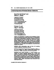
0 0 Ts2 2 1
where m = a / x 2 + y 2 , a = 2, x and y represent component of the velocity at the current moment, respectively. In the implement of DAPF, we use N = 200 particles and 200 sensors. In Figure 1, we can see the sensors are displayed with small circles and the head nodes are displayed with small star. In the addition, the true trajectory and the track trajectory is displayed with the solid line and dotted line, respectively. It can be seen that the algorithm track the target’s trajectory closely, so the algorithm we proposed is effective. In Figure 2, we can see the simulation time-consuming comparison of three algorithms (centralised particle filtering, DPF and DAPF). It is clear that DAPF’s time-consuming is significantly less than the centralised particle filtering’s and DPF’s in the case of the same number of particles. At the same time, with the number of particles increasing, DAPF has the same time-consuming.
Target tracking of binary wireless sensor networks in the domain of medicine and healthcare It is because the number of used particles during filtering can be changed according to the real filtering situation. Considering the specificity of WSN, communication amount is the important indicator to measure the effectiveness of the algorithm. We use the same method as in Sheng et al. (2005) to estimate communication amount but change some parameters. The communication amount can be estimated by
Ne N f + 3cNc N s N f + N n Ni where Nf = 16, Ni = 8, Nc = 1, Nn = 1, Ne represent the number of nodes within the cluster, Ns represent the dimension of the state variables. In this paper, we set Ns = 4. Figure 1
Target tracking with DPAF
Table 1
193
Comparison of communication amount of three algorithms (bits)
Number DPF
100
200
400
900
141,618
256,789
512,783
1,095,191
GMM-DPF
9266
8469
8463
8087
DAPF
3634
3349
3343
3223
6
Conclusions
Target tracking is the important application of WSN. But the characteristics of WSN limit the traditional tracking algorithm. To accurately track target in WSN, in this paper, we focus on the use of DAPF for target tracking in binary WSN. Extensive simulations of this algorithm performed under different configurations. From the simulations, we can see our algorithm can track the target accurately, and reduce the communication amount and the energy consumption. Therefore, DAPF is an effective algorithm and more fit for WSN.
Acknowledgements The paper is supported in part by the Natural Science Foundation of Beijing under the Grant No. 4122073.
References
Figure 2
Comparison of time-consuming of three algorithms
In Table 1, we can see the traffic comparison of three algorithms. We can see from the table that DAPF’s traffic is the least in these algorithms. From above all, we can see our algorithm yields good performance and outperforms other algorithms.
Coates, M. (2004) ‘Distributed particle filters for sensor networks’, Information Processing in Sensor Networks IPSN2003, Springer, pp.99–107. Ding, M., Yang, D., Zhuang, L. and Li, X. (2013) ‘Navigation algorithm for WSN mobile node on MH particle filtering improvement’, International Journal of Sensor Networks, Vol. 14, No. 2, pp.92–101. Djuric, P.M., Vemula, M. and Bugallo, M.F. (2008) ‘Target tracking by particle filtering in binary sensor networks’, IEEE Transactions on Signal Processing, Vol. 56, No. 6, pp.2229–2238. Gao, W., Zhao, H., Song, C. and Xu, J. (2009) ‘A new distributed particle filtering for WSN target tracking’, International Conference on Signal Processing Systems, May, pp.334–337. Gasparri, A., Panzieri, S., Pascucci, F. and Ulivi, G. (2009) ‘An interlaced extended Kalman filter for sensor networks localisation’, International Journal of Sensor Networks, Vol. 5, No. 3, pp.164–172. Ghirmai, T., Kotecha, J.H. and Djuic, P.M. (2004) ‘Blind equalization for time-varying channels and multiple samples processing using particle filtering’, Digital Signal Processing, Vol. 14, pp.312–331. Gustafsson, F., Gunnarsson, F., Bergman, N., Forssell, U., Jansson, J., Karlsson, R. and Nordlund, P-J. (2002) ‘Particle filters for positioning, navigation, and tracking’, Signal Processing, IEEE Transactions on, Vol. 50, No. 2, February, pp.425, 437.
194
S. Ling-Dong et al.
Hao, Q., Hu, F. and Xiao, Y. (2009) ‘Multiple human tracking and identification with wireless distributed pyroelectric sensor systems’, IEEE System Journal, Special Issue on Biometrics, Vol. 3, No. 4, December, pp.428–439. Huang, Y., Liang, W., Yu, H-B. and Xiao, Y. (2008) ‘Target tracking based on a distributed particle filter in underwater sensor networks’, (Wiley) Wireless Communications and Mobile Computing (WCMC), John Wiley & Sons, Vol. 8, No. 8, October, pp.1011–1022. Lattanzi, E. and Bogliolo, A. (2014) ‘Hardware filtering of non-intended frames for energy optimisation in wireless sensor networks’, International Journal of Sensor Networks, Vol. 15, No. 2, pp.121–129. Lin, J., Xie, L. and Xiao, W. (2009) ‘Target tracking in wireless sensor networks using compressed Kalman filter’, International Journal of Sensor Networks, Vol. 6, Nos. 3–4 pp.251–262. Niu, R. and Varshney, P. (2004) ‘Target location estimation in wireless sensor networks using binary data’, Presented at the 38th Annu. Conf. Inf. Sci. Syst., Princeton, NJ. Ozdemir, O., Niu, R. and Varshney, P.K. (2006) ‘Channel aware particle filtering for tracking in sensor networks’, Proc. Asilomar Conf. Signals, Systems, Computers, Pacific Grove, CA, October. Ozdemir, O., Niu, R. and Varshney, P.K. (2009) ‘Tracking in wireless sensor networks using particle filtering: physical layer cansiderations’, IEEE Transactions on Signal Processing, Vol. 57, No. 5, pp.1987–1999. Peng, M. and Xiao, Y. (2012) ‘A survey of reference structure for sensor systems’, IEEE Communications Surveys & Tutorials, Vol. 14, No. 3, Third Quarter 2012, pp.897–910.
Peng, M. and Xiao, Y. (2010) ‘Signature maximization in designing wireless binary pyroelectric sensors’, Proceedings of the IEEE Global Telecommunications Conference 2010. Miami, Florida, USA, December, pp.1, 5, 6–10. Peng, M., Xiao, Y., Li, N. and Liang, X. (2014) ‘Monitoring space segmentation in deploying sensor arrays’, IEEE Sensors Journal, Vol. 14, No. 1, January 2014, pp.197–209. Ren, H. and Meng, M.Q-H. (2009) ‘Power adaptive localization algorithm for wireless sensor networks using particle filter’, IEEE Transactions on Vehicular Technology(2009), Vol. 58, No. 5, pp.2498–2507. Sheng, X.H., Hu, Y.H. and Ramanathan, P. (2005) ‘Distributed particle filter with GMM approximation for multiple target s localization and t racking in wireless sensor network’, Proc of 4th Int. Symposium on Information Processing in Sensor Networks, ACM Press, Los Angeles. Wang, Z., Bulut, E. and Szymanski, B.K. (2008) ‘Distributed target tracking with imperfect binary sensor networks’, Proceedings of the Second Annual Conference of the International Technology Alliance, London UK, pp.306–307. Yang, H. and Sikdar, B. (2003) ‘A protocol for tracking mobile targets using sensor networks’, Proceedings of IEEE SNPA(2003), pp.71–81. Zhang, M., Hu, J-w., Peng, J-p. and Zhou, Y-f. (2009) ‘A new adaptive particle filtering algorithm’, Command Control and Simulation(2009),Vol. 31, pp.39–44. Zuo, L., Mehrotra, K., Varshney, P. and Mohan, C. (2006) ‘Bandwidth-efficient target tracking in distributed sensor networks using particle filters’, Proc. of 14th European Signal Processing Conference EURASIP2006, September, Florence, Italy.