Teaching Bayesian Model Comparison With the ... - Stanford Statistics

Teaching Bayesian Model Comparison With the Three-sided Coin Scott R. Kuindersma

Brian S. Blais∗,†

Department of Science and Technology, Bryant University, Smithfield RI January 4, 2007 Abstract In the present work we introduce the problem of determining the probability that a rotating and bouncing cylinder (i.e. flipped coin) will land and come to rest on its edge. We present this problem and analysis as a practical, nontrivial example to introduce the reader to Bayesian model comparison. Several models are presented, each of which take into consideration different physical aspects of the problem and the relative effects on the edge landing probability. The Bayesian formulation of model comparison is then used to compare the models and their predictive agreement with data from hand-flipped cylinders of several sizes. Keywords: probability theory, log-likelihood, parameter estimation, marginalization, Occam’s razor.

1. INTRODUCTION The success of Bayesian inference has led to a paradigm shift in our understanding of statistical inference based on a theory of extended logic. In light of this paradigm shift, it is important to introduce students to the fundamentals of Bayesian probability theory and its wide range of applications. Bayesian probability theory is a unified approach to data analysis that encompasses both inductive and deductive reasoning(Gregory, 2005). The Bayesian approach to model comparison offers a straightforward and effective solution to the problem of model selection. From a simple application of Bayes’ Theorem, we are able to assign a probability to each model and compare them directly with one another. Here we apply this technique to the problem of the three-sided coin. A three-sided coin is defined to be a cylinder that, when flipped like a coin, has some possibly non-negligible probability of landing on its edge. An ideal coin has a probability of 0.5 for landing on heads, or tails, due to the symmetry (the limit of the edge height going to zero). Once the edge height is allowed to be finite, factors such as geometry and flip dynamics become significant. Several models are presented that assign probabilities for a coin landing on edge, each taking into account different aspects of the problem. The first four models focus only on the geometrical constants of the coin(Mosteller, 1987; Pegg, 1997), containing no free parameters, while Models 5 and 6 are statistical models with free parameters. Each model is compared to data on hand-flipped cylinders of various sizes. The likelihood of each model given the data is calculated using Bayesian model comparison and it is shown that the statistical models perform better than the purely geometrical ones. We also illustrate how this type of analysis allows us to question assumptions made by a model and how relative complexity plays a significant role in the probabilities assigned to the models. This problem is a particularly good one for teaching probability and statistics, especially from a Bayesian perspective. The data are easily obtained in a class or lab setting, there is a number of models of varying complexity ∗ also

at Institute for Brain and Neural Systems, Brown University, Providence RI author

† Corresponding

1

h

R

R 2α

2β

h

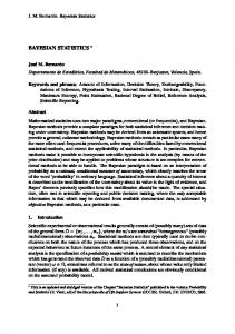
l Figure 1: Three-sided coin. (A) A cylinder with radius, R, of the circular cross section and height, h, of the edge. (B) The cross section of the cylinder, with internal angles, α and β, and length, l, defined. that can be explored, and there is no “right” answer, which students can refer. As a result, there is a lot of flexibility in examining the three-sided coin. We restrict ourselves here to models with relatively simple physics concepts, to keep the focus on model selection and to not imply that a physics background is necessary to use the three-sided coin in a teaching setting.

2. THE THREE-SIDED COIN The coin is represented by its rectangular cross section, as shown in Figure 1. The important geometrical quantities used in the models presented are the following:

ratio of the edge height to the radius,

η

the diagonal length of the coin, l internal angle (see Figure 1), β internal angle (see Figure 1), α

≡ h/R p ≡ R2 + (h/2)2 ≡ atan(η/2) ≡ atan(2/η)

We will ask the question What is the probability, pedge , for the coin to land (and come to rest) on the edge, as a function of the radius, R, and the height, h? The models presented attempt to answer this question by considering different aspects of the problem. For the geometrical models (Models 1-4) this will involve no further parameters or concepts other than the geometrical constants of the coin. The statistical models (Models 5 and 6) will consider the effect of bouncing in addition to the cylindrical geometry.

3. MODELS OF THE THREE-SIDED COIN In this section we describe five models of the three-sided coin that focus on different aspects of the problem in order to assign a probability to an edge landing.

2

3.1

Model 1: Surface Area

In analogy with dice, one presumes that the probability is proportional to the surface area of the edge.

3.2

pedge (h, R)

=

pedge (η)

=

2πRh 2πR2 + 2πRh η 1+η

Model 2: Cross-sectional Length

Again, in analogy with dice, one presumes that the probability is proportional to the cross-sectional length. A square cross section would assign equal probabilities to all sides.

3.3

pedge (h, R)

=

pedge (η)

=

h 2(2R) + h η 4+η

Model 3: Solid Angle

It has been suggested(Mosteller, 1987; Pegg, 1997) that the probability of landing on a given side of a three-sided coin is proportional to the solid angle subtended by the side. For the edge probabilities we obtain 2π

Z edge area subtended

=

Z

0

pedge (η)

3.4

π/2+β

dφ

sin θdθdφ π/2−β

= 4π sin β = sin β η = p 2 η +4

Model 4: Center of Mass

For a solid object with one point of contact with the floor, the location of the center of mass with respect to the vertical line through the contact point determines which way the object will tip. If we assume there is no bouncing, then the angle, θ, at which the coin comes in contact with the floor will entirely determine the final resting configuration. • if 0 < θ < α then the coin will land on heads (i.e. heads-conducive) • if α < θ < π/2 then the coin will land on the edge (edge-conducive) Therefore the probability for landing on edge is simply pedge (h, R) = 1 − where we define pe for use in later models.

3

α ≡ pe π/2

(1)

Center of Mass Energy

1

Ee=0.2

Eh=0.8

R

0.5 h/2 0 0

π Angle

π/2

3π/2

2π

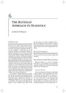
Figure 2: The energy values used in the Simple Bounce model. The blue line traces the center of mass of a cylinder relative to a flat surface as it is rotated 360 degrees.

3.5

Model 5: Simple Bounce

The Simple Bounce model takes the effect of bouncing into consideration. Bouncing is incorporated in the following way. Let E be the incoming energy of the coin as it falls, and γ be the fractional energy loss on each bounce, i.e. on each bounce E → γE. For example, if E = 100 and γ = 0.2, then the value of E after two bounces would be γ 2 E = 4. At each bounce, we consider the location of the center of mass as the coin makes contact with the solid surface, as in Model 4. We also define two constant energy values Eh Ee

≡ l − h/2 ≡ l−R

where Eh is the minimum energy needed to bounce out of the heads (or tails) state. Similarly Ee is the minimum energy needed to escape the edge state (Figure 2). We will assume that as long as the coin has enough energy to escape these states, it will continue randomizing its angle. Eventually it will not have enough energy to escape one of the states and will come to rest in that state. We can further illustrate this point using simple numbers. Lets say that for some coin the current energy, E = 50, and γ = 0.1, with well depths Eh = 0.8 and Ee = 0.2. On the first bounce, the energy will drop to E = 5, which is larger than both energy wells, and thus the coin will escape and re-randomize. The second bounce yields E = 0.5, which is smaller than the energy well for the heads state but larger than the one for the edge state. If the bounce was heads-conducive, then the coin will come to rest in the heads state. If the bounce was edge-conducive, it will escape the state and re-randomize. In this case, the next bounce yields E = 0.05, and a further edge-conducive bounce will bring the coin to come to rest in the edge state. By examination, one can see that, in general (for h/R < 2), Ee is smaller than Eh . There will come a point when the energy will be large enough to escape the edge state, but not a heads or tails state. After that point, if the coin has a heads-conducive fall, then it will remain in the heads state forever, coming to rest on heads. Thus, to come to rest on edge, the coin must have a series of edge-conducive falls in a row until the energy falls to the point where it cannot escape the edge state (γE < Ee ). We take the probability for an edge-conducive fall, pe , from Model 4, Equation 1. If we start with energy just able to escape the largest state (Eh ), and bounce until we cannot escape the smallest state (Ee ), then we will bounce 4

n times where n is n = log(Ee /Eh )/ log γ + 1

(2)

The probability of bouncing n times, each time with an edge-conducive fall, is simply pedge = pne

(3)

It is worth noting that there are several assumptions made in this model which may or may not be correct. Perhaps the three most important of these assumptions are 1. the initial energy has a negligible effect 2. the coin’s angle is randomized after each bounce 3. the fractional energy loss γ is the same at each bounce As we shall see, the analysis using Bayesian model comparison will be useful in determining whether we should reconsider one or more of these assumptions.

3.6

Summary of Models

Figure 3: Summary of Models 1-5. The five models are summarized in Figure 3. The Simple Bounce model (Model 5) gives a much lower probability of edge landing for thin coins than the purely geometrical models (Models 1-4). This seems to be more closely aligned with one’s intuition. Table 1 shows us that the edge-landing probabilities assigned to US coins by Models 1-4 are much too large.

5

Model M1 : Surface Area M2 : Cross-sectional Length M3 : Solid Angle M4 : Center of Mass M5 : Simple Bounce

Nickel 1/6 1/23 1/11 1/17 1/226890

Quarter 1/8 1/29 1/14 1/22 1/1699613

Penny 1/7 1/26 1/12 1/19 1/614281

Dime 1/8 1/28 1/13 1/21 1/1167291

Table 1: Predicted probabilities of U.S. coins landing on edge when flipped. For Model 5, the free parameter γ = 0.2.

Figure 4: Data from coin flips, using PVC solid stock.

6

1 inch h/R 0.43 0.84 1.03 1.29 1.53 1.66

Flips 200 200 200 200 200 200

2 inch

Edge Landings 1 48 58 74 120 118

h/R 0.25 0.50 0.75 1.25 2.00

Flips 100 100 100 105 100

Edge Landings 1 5 13 28 61

Table 2: Data from flipping experiments with 1 and 2 inch diameter PVC coins.

4. EXPERIMENTAL RESULTS Experiments were done with solid PVC stock cut into cylinders of different sizes. Flips were done in a vigorous way onto tile floor, excluding those bounces which carried the coin out of a 1ft square. This exclusion was to make sure that flips which gave coins a significant roll would not be counted. This effect could, of course, later be examined to determine its significance. The data is shown in Figure 4. The error bars denote the 95% credible intervals for the probability estimates. Table 2 describes the data in further detail.

5. MODEL COMPARISON In the Bayesian formulation of model selection we start with the calculation of posterior probabilities for the models, Mi , given the data, D, and any other information, I (Jaynes, 2003) P (Mi |D, I) =

P (Mi |I)P (D|Mi , I) P (D|I)

and look at their ratios to examine the relative probabilities for each model (i.e. the odds of one model to another) P (Mi |I)P (D|Mi , I) P (Mi |I)L(Mi ) P (Mi |D, I) = = P (Mj |D, I) P (Mj |I)P (D|Mj , I) P (Mj |I)L(Mj ) If we assign equal prior probabilities to each model (P (Mi |I)/P (Mj |I) = 1), then the ratios of the posteriors becomes simply the ratios of the likelihoods, L(Mi )/L(Mj ). For convenience we use the log of the likelihood and compare the differences log P (Mi |D, I) − log P (Mj |D, I) = log L(Mi ) − log L(Mj ) We are able to calculate the log-likelihoods for Models 1-4 directly using the binomial probability distribution and summing over all data points X log L(Mi ) = log n! − log r! − log(n − r)! + r log p + (n − r) log(1 − p) where n is the number of flips, r is the number of edge landings, and p is the probability of landing on edge as predicted by model Mi . Since Model 5 has a free parameter, γ, we must marginalize over that parameter to attain the likelihood. The parameter γ is a continuous variable, so marginalization takes the form of integration Z L(M5 ) = dγp(γ|M5 , I)p(D|γ, M5 , I) 7

Model Model 1: Model 2: Model 3: Model 4: Model 5:

Surface Area Cross-sectional Length Solid Angle Center of Mass Simple Bounce

Log-likelihood -229 -162 -155 -91 -78

Table 3: Log-likelihoods for three-sided coin models on the data from PVC solid stock. These values are sorted from least likely (smallest likelihood) to most likely (largest likelihood), given the data.

using the notation of (Gregory, 2005). This has the benefit of automatically penalizing more complex models unless the additional complexity can be justified with a significantly better fit (i.e. a quantitative Occam’s razor)(Loredo, 1990). We assume γ to be continuous over some range where each value is equally likely to be the actual value of γ. We therefore assign a uniform prior probability density function (PDF) Z dγp(γ|M5 , I) = p(γ|M5 , I)∆γ = 1 ∆γ

 p(γ|M5 , I)

=

1 ∆γ

0

when γmin < γ < γmax , otherwise.

where ∆γ is the width of the prior PDF (γmax − γmin ). The marginalization is performed numerically, with a simple brute-force algorithm. The range used for γ a priori is [0, 0.5]. From the PVC solid stock data we calculate the log-likelihoods shown in Table 3. Recall that larger log-likelihoods imply a model is more likely given the data, and each increment in value is a factor of e difference in the posterior probability. From this table we can see that the Simple Bounce model is the most probable given the data. However, if we look at the posterior PDF for γ shown in Figure 5, we see that there is a problem with the model. The most likely value for γ taken from the posterior (the maximum of the curve shown in Figure 5) is approximately 0.0001, which yields, using Equation 2, an average number of bounces of 1.16 (i.e. no bounces after first impact), which is not what is observed empirically. If, instead of the maximum of the posterior, we use the median, then we can calculate credible intervals to quantify the uncertainty. By definition, we are 95% certain that the parameter has the values within the 95% credible interval. In the case of estimating γ, we obtain an estimate (from the median) of γ = 0.0005, with a 95% credible interval of [0.00006, 0.002383]. This does not change our conclusions, but is included here for completeness. The point of this is to demonstrate that the estimation of the parameters, and the uncertainty in those estimates, is a straightforward process. In further estimates, we will adopt the convention of displaying the median and the 95% credible intervals. With this new information, we now go back and reconsider the assumptions of the Simple Bounce model. In doing so, we will be able to formulate an alternative bounce model. As we mentioned above, the Bayesian model comparison technique acts like a quantitative Occam’s Razor by penalizing more complex models, assigning them larger probabilities only if the additional complexity is justified by a significantly better prediction of the observed data. What we generally mean by “additional complexity” are additional free parameters and/or wider or more uniform prior PDFs for parameters. This penalty is a direct result of the marginalization performed on the free parameters. We can demonstrate this effect by modifying the width of the prior PDF (∆γ) in Model 5. If we do the same analysis as above with the prior ranges for γ equal to [0, 0.1] and [0, 0.9], the log-likelihood for the model becomes −76.05 and −78.25, respectively. This about a factor of 6 difference in posterior probability. 8

Figure 5: The posterior probability density function for Model 5 parameter γ.

6. MODEL 6: NEW SIMPLE BOUNCE With this new model we reconsider some of the assumptions made in the original Simple Bounce model. The third assumption of the Simple Bounce model was that the fractional energy loss, γ, is the same for both heads-conducive and edge-conducive bounces. However, the difference between these energy losses could be significant. We now try using two separate parameters, γe and γh . We make no assumption about which γ is larger and we use the same prior range for each, [0, 0.5]. Note that we could have added an arbitrary number of γ parameters that would correspond to different energy losses for different bounce angles, but this additional complexity would make it computationally prohibitive, and would incur a significant Occam penalty. We therefore add only one additional bounce parameter and consider the possibility of additional parameters only if the results from the analysis are unsatisfactory. In Model 5, we made use of the energy values Eh and Ee . We will continue to use these values as well as the center of mass method (pe ) to determine whether a landing is heads or edge-conducive. We remove the initial energy assumption by randomizing the initial value of E. Starting with a random energy E taken from some range ∆E, we simulate n flips of a coin, keeping track of the resting state of each flip. The probability is then taken as the ratio of edge landings to total flips pedge =

nedge n

We maintain the assumption that the coin will continue randomizing its angle on each bounce because there does not seem to be any reasonable and simple alternative.

6.1

Model 6 Analysis

After we run the flipping simulations we marginalize over the three free parameters, γe , γh , and E with uniform prior ranges of [0, 0.5], [0, 0.5], and [1, 5], respectively. For parameter estimates, we calculate the full posterior, and 9

marginalize over all other parameters, and the log-likelihood is also calculated by marginalizing over the parameters. Using these procedures, we arrive at a log-likelihood of −50. That is a great improvement over the original Simple Bounce model, but we also want to examine the marginal posteriors for each γ parameter to make sure the values are indeed reasonable. Given the PVC data, the best estimate (from the median) and the 95% credible intervals of the values of γh and γe are 0.496 ([0.458, 0.537]) and 0.090 ([0.078, 0.102]), respectively. In this model, the average number of bounces is 2.0, which is more physically meaningful than the values obtained from Model 5. Assuming independence of the parameters is a computational convenience, and would not affect the results significantly.

7. DISCUSSION In the initial analysis (of Models 1-5), it was clear that Model 5 was the most likely model, given the data. However, the examination of the posterior for γ prompted us to reconsider the model because the most likely value of γ was far too small to be physically reasonable. We were then able to formulate a New Simple Bounce model which addressed some of the assumptions made in the original Simple Bounce model. However, in doing so we added additional complexity to the model. But after calculating the log-likelihood for the New Simple Bounce model we are able to say that the additional complexity is indeed justified because it performs far better than the other models, given the data. A similar problem is addressed in (Dunn, 2003), where instead of a cylinder, a series of rectangular dice that differ in length are used. These 1 × 1 × r dice (or η ≡ 2r, in our notation) are rolled and the results analyzed with generalized linear models. Using this data (we chose their more careful “Group A” data), we are not surprised that Model 6 once again performs better than the other models. Additionally, we would expect there to be differences in the bouncing and rolling properties of rectangles and cylinders. These are observed in the estimates of the bounce parameters (see Table 4).1 One can then go further to explore more details of the physics, using whatever data one wishes, applying the straightforward model comparison techniques described here. The Bayesian approach has the advantage over the regression from (Dunn, 2003) in that one can easily apply it to parameters of physical interest, with straightforward interpretation. It is not only predictive in the current experimental setup, but can guide the experimenter to other aspects of the problem that might be important, and guide him or her away from aspects that are not important. We have shown that Bayesian model comparison not only helps us choose the best model for predictive purposes, it also allows us to identify which features of the problem are more significant than others. This information can then be used to refine existing models or formulate new ones. We can now say with confidence that models of the three-sided coin must go beyond the geometrical constants of the coin and include some dynamical properties. Using Bayesian analysis we are able to approach the three-sided coin problem making simple assumptions then refine our model incrementally, eventually leading us to a workable model with minimal complexity.

References Dunn, Peter K. (2003). What Happens When a 1x1xr Die is Rolled? American Statistician, 57(4):258–264. Gregory, P. (2005). Bayesian Logical Data Analysis for the Physical Sciences. Cambridge University Press, New York, NY, USA. Jaynes, E. T. (2003). Probability Theory: The Logic of Science. Cambridge University Press, Cambridge. Edited by G. Larry Bretthorst. 1 If we include the unpublished data from Dan Murray at www.geocities.com/dicephysics/3sided.htm using a machine to flip (N ∼ 50, 000), our results are still maintained, with qualitatively similar parameter estimates.

10

A Model Model Model Model Model Model Model

1: 2: 3: 4: 5: 6:

Surface Area Cross-sectional Length Solid Angle Center of Mass Simple Bounce New (2-γ) Bounce

Log-likelihood Kuindersma-Blais Dunn, 2003 -229 -287 -162 -876 -155 -178 -91 -346 -78 -165 -50 -121

B Model Model 5: Simple Bounce, γ Model 6: New (2-γ) Bounce, γh Model 6: New (2-γ) Bounce, γe

Kuindersma-Blais Median 95% Credible Region 0.0005 [0.00006, 0.0024] 0.496 [0.458, 0.527] 0.090 [0.078, 0.102]

Median 0.159 0.756 0.296

Dunn, 2003 95% Credible Region [0.143, 0.172] [0.736, 0.779] [0.271, 0.319]

Table 4: (A) Log-likelihoods for three-sided coin models on the data from PVC solid stock (Kuindersma-Blais) and 1 × 1 × r rectangular dice (Dunn, 2003). (B) Parameter estimates for the bounce parameters for the same data sets. Shown are the median value, and the 95% credible region around the median.

Loredo, T. J. (1990). From Laplace to supernova SN 1987A: Bayesian inference in astrophysics. In Fougere, P., editor, Maximum Entropy and Bayesian Methods, Dartmouth, U.S.A., 1989, pages 81–142. Kluwer. Mosteller, F. (1987). Fifty Challenging Problems in Probability with Solutions. Dover Publications. Pegg, E. (1997). A Complete List of Fair Dice. Masters Thesis.

11