Teaching Special Relativity Using Physlets® Mario Belloni, Wolfgang Christian, Davidson College, Davidson, NC Melissa H. Dancy, Western Carolina University, Cullowhee, NC
I
n a recent paper in this journal1 we presented work on the creation and use of Physlet-based2 exercises to teach physical and wave optics. Since then we have developed ready-to-run exercises for introductory physics3, 4 and have developed Physletbased exercises for more advanced topics such as quantum mechanics. In this paper we describe the materials we have created to aid in the teaching and learning of introductory special relativity. There are many reasons to focus on special relativity. Special relativity is the first topic presented in the modern physics section of introductory physics courses and in the sophomore-level modern physics course. It is full of (apparent) paradoxes, and like quantum mechanics, is one of the intriguing theories that continues to captivate students’ interest in physics. In addition, because special relativity focuses on abstract concepts, the visualization that Physlet-based material provides is especially valuable.
Motivation Recent work by Scherr5,6 and her collaborators determined student-held beliefs about the relativity of simultaneity and created paper-and-pencil exercises to aid student understanding of relativity. Their research, which goes hand-in-hand with commentary by others,7,8 reveals that the teaching of introductory special relativity should focus less on the Lorentz transformations and more on the relativity of simultaneity, length contraction, and time dilation. Several textbook authors have already taken this approach.9–12 A focus on Lorentz transformations can 8
obscure the fact that special relativity is about spatial and temporal intervals and not about single position measurements and clock readings. In addition, an approach based on spatial and temporal intervals leads to the metric in special and general relativity while Lorentz transformations do not. In our experience, pencil-and-paper exercises alone are often insufficient to aid student understanding of abstract ideas, such as those in special relativity. We believe that the level of visualization and interactivity of carefully constructed Physlet-based exercises offers students a distinct learning advantage over such traditional exercises.13 While there are other computer programs that simulate phenomena in special relativity, most notably “Spacetime” and “RelLab,”14 Physlets are free for noncommercial use and Physlet-based curricular material can be written to specifically target concepts that students find difficult. Because our material is web-based, it is flexible enough to be adapted to a variety of pedagogical strategies and local environments. Finally, since Physlet-based material exists for all topics in introductory physics, students can use the same material throughout the course, rather than being forced to become familiar with numerous software packages. For special relativity, we have incorporated the results from Scherr’s physics education research into our development of several interactive Physlet-based exercises that focus on visualizing the relativity of simultaneity, length contraction, time dilation, and spacetime diagrams. These exercises can be used as interactive reading assignments, in-class demonstraTHE PHYSICS TEACHER ◆ Vol. 42, May 2004
tions, interactive tutorials, and as part of an introductory physics laboratory in special relativity. The material described in this paper and the laboratory version of these exercises can be found at http://webphysics. davidson.edu/physlet_resources. A brief description of each exercise follows.
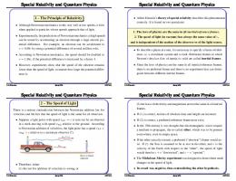
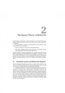
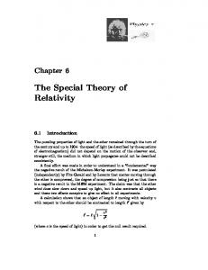
the origin. This time delay allows all of the clocks to be synchronized by the use of a light pulse emitted from the master clock at a time of our choosing. We know that for every 1 m a clock is displaced from the master clock, there is going to be 1 m of light traveltime (or 3.33 x 10⁻⁹ seconds) delay, and so we preset each clock to account for this delay. Every tick of a Examples of Curricular Material clock, therefore, also represents the time it takes light Creating a Spacetime Lattice to travel one meter. In Fig. 1(a), the pulse has not yet been emitted and the grayed-out clocks are not yet running. Once the student plays the animation, a (a) light pulse (shown in red) is emitted from the master clock, the pulse eventually reaches a clock, and the clock turns on as shown in Fig. 1(b) and 1(c). This process continues until all of the clocks are on and the result is that all of the clocks are synchronized. Since students see the result of the creation of the spacetime lattice, they better understand what it (b) means. We also point out that while we have drawn a one-dimensional, finite-size reference frame on the screen, the reference frame is actually three dimensional and of infinite extent. The follow-up exercise shown in Figure 2 points (c) out that there is an important distinction between an observer who constructs a spacetime lattice and a viewer who sees the lattice from a fixed point in space.9 As a consequence, what an observer records Fig. 1. One method for visualizing clock synchronizaafter the synchronization of clocks is not what a viewtion. er of the clocks would see. This is a common misunNo discussion of special (or even Galilean) relatividerstanding in special relativity. What we depict in ty can begin without the introduction of a reference setting up a reference frame is what an omnipresent frame in which to perform measurements. Reference (or intelligent5,6) observer would record in a laboratoframes and their creation are nonetheless difficult constructs for students to understand. To aid student understanding of reference frames, we developed a Physlet-based exercise that builds one (we do so in on(a) ly one spatial dimension for simplicity). When the applet is initialized, a spatial grid with gridlines placed at 1-m increments is shown. To make this grid a spacetime lattice, we also place a set of clocks at each gridline to be synchronized with a master clock. One synchronization procedure is depicted in Fig. (b) 15 1. Figure 1(a) shows a spacetime lattice with numerous clocks, which is what a student sees before playing the animation. Each clock is separated by 1 m Fig. 2. Synchronized clocks factoring in light-travel time from its nearest neighbors and a time delay is built indelay. In Fig. 2(a) the viewer is at the origin, while in Fig. 2(b) the viewer is 100 m out of the page in the z to all clocks, with the exception of the master clock at direction. THE PHYSICS TEACHER ◆ Vol. 42, May 2004
9
ry notebook This description leads to the idea of a Schwarzschild bookkeeper in general relativity. Often students (and physicists alike) mistakenly believe that the strange things that are a part of special relativity are due to light-travel time delay. They are not! A nearby viewer would not see all of the clocks synchronized because of the light travel-time delay. Instead the viewer would see what is depicted in Fig. 2(a) where the viewer has not factored in the light travel-time delay. In this exercise students can change the position of the viewer in both the x (left and right) and z (out of the page) directions. In Fig. 2(b) the viewer is 100 m out of the page on the z axis. Note that far away from the clocks, even with the light travel-time delay, all of the clocks appear to be approximately synchronized. The Relativity of Simultaneity
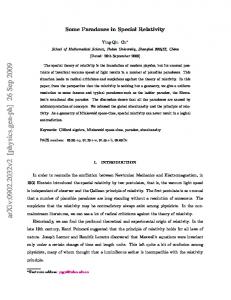
In this example, a lightning bolt hits the center of a flatbed railcar at t = 0 seconds as shown in Fig. 3(a)
(a)
(b)
(c)
Fig. 3. Two different experiments illustrating the relativity of simultaneity.
10
(position is given in meters and time is given in seconds). There is a relative velocity between the reference frame of the ground (labeled S) and the reference frame of the railcar (labeled S'). When the animation runs, students see the relative motion of either the railcar or the ground depending on which experiment they choose. In addition, the light from the lightning strike is shown in red as an expanding circle and as time goes on the light eventually reaches all of the observers (labeled A, B, A', and B'). In the animation called “Experiment 1: From the Frame of the Ground” shown in Fig. 3(b), the event of the lightning strike and the subsequent transmission of this information are shown as seen from the reference frame of the ground. Alternatively, in “Experiment 2: From the Frame of the Railcar” shown in Fig. 3(c), a similar, but not the same, experiment is depicted as seen from the reference frame of the railcar. In “Experiment 1” [Figure 3(b)], the railcar is moving to the right at a given speed as depicted in the lower panel by S' moving to the right. As the circle representing the path of a spherical light wave expands, it first encounters the observer (the man) at A'. Next, the outgoing spherical light wave reaches the observers at A and B simultaneously. Finally, the light reaches the observer at B'. In “Experiment 2” [Fig. 3(c)], as the red circle representing the path of a spherical light wave expands, it first encounters the observer (the woman) at B. Next, the outgoing spherical light wave reaches the observers at A' and B' simultaneously. Finally, the light reaches the observer at A. This animation therefore visually illustrates for students that simultaneity is relative by showing that the light reaches the observers in a different order in the two frames. Note that there are two different experiments depicted, each with a different railcar and a different set of observers. To see why this must be the case we first need to discuss length contraction. Time Dilation and Length Contraction with Light Clocks
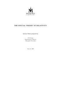
One of the best ways to visualize time dilation and length contraction is with the construction of a light clock. A light clock consists of a box with a light pulse emitter and light detector on its bottom wall and a mirror on its top wall. Light is emitted from the bottom wall and every time the light pulse returns to the THE PHYSICS TEACHER ◆ Vol. 42, May 2004
Fig. 4. Vertical light clocks with a relative velocity of  = 0.866. Note that in all panels, the light pulses from the red clock and the green clock have traveled the same distance. In the top right panel, the light pulse of the red clock has traveled up and down once. In the lower right panel, the light pulse of the red clock has now traveled up and down twice, while the light pulse of the green clock has traveled up and down only once.
bottom wall, the detector triggers a tick of the clock, and another flash is emitted. In the animation, the light pulse is shown as either a red or green circle and its path is shown as a faint red or green trail. The distance between the top and bottom walls is 0.5 m, and therefore, the total vertical trip distance between clock ticks is 1.0 m. Given this, the clocks read time in meters. Since light travels 1 m every 3.33 x 10⁻⁹ seconds, every tick of the clock represents the time it takes for light to travel 1 m or 3.33 x 10⁻⁹ seconds. Most textbooks have a figure similar to that of Fig. 4, but our example is animated and also allows students to vary the speed of the moving light clock. Students choose a relative velocity (the figures here use  = v/c = 0.866 and hence ␥ = 1/(1 – 2)1/2 = 2) and run the animation. A stationary observer relative to the moving light clock sees the moving clock tick more slowly than the stationary clock because the time interval between ticks of the moving clock is seen to be longer compared to the stationary clock. This is time dilation. Figure 4 shows that the moving clock ticks half as often as the stationary one (the time interval between ticks for the moving clock doubles). This result occurs for the light clock because the speed of light is constant in any reference frame, therefore, the distances traveled by the two light pulses must be the same as viewed in the frame of the stationary clock. THE PHYSICS TEACHER ◆ Vol. 42, May 2004
Fig. 5. Horizontal light clocks with a relative velocity of  = 0.866. Note that in all panels, the light pulses from the red clock and the green clock have traveled the same distance. In the top right panel the light pulse from the red clock has traveled back and forth once, while in the lower right panel the light pulse from the red clock has traveled back and forth twice.
However, the distance traveled by the moving clock involves both horizontal and vertical components, and it is only the vertical component of the light pulses’ motion that contributes to the clock ticks.17 In the second animation, the light clocks are tilted sideways. Since the temporal slowing of the moving clock must still occur for the sideways clock and the speed of light is unchanged, the distance between the walls of the moving clock must now be contracted. In fact, for  = 0.866, it must be contracted to half its rest length as shown in Fig. 5. This is length contraction. Spacetime Diagrams
One of the most useful ways to visualize moving objects in special relativity is with spacetime diagrams. In this exercise, students step through the following progression (not shown) dealing with a woman walking at a constant velocity.
»
» »
Animation 1: The motion of the woman is plotted on
a position versus time graph. The speed of the woman can be determined by the slope of the position versus time graph. Animation 2: In this animation, time is plotted versus position. The graph is the same as Animation 1 with the axes flipped. Animation 3: This animation puts time on an equal footing with position. What has been done is to multiply time by the speed of the woman. Therefore, vt is plotted versus position. This converts the unit of time into meters. 11
Fig. 6: Spacetime diagrams for a woman with a  of 0, 0.9, and -0.9.
»
Animation 4: For a true spacetime diagram, we
multiply the time by the speed of light. The unit of the y axis now becomes the amount of time it takes for light to travel 1 m, or 3.33 x 10⁻⁹ seconds. By slowly stepping students through the procedure described above, they see that the spacetime diagram is not too far removed from the familiar position versus time graph. Demystifying spacetime diagrams is the first step in being able to use this powerful tool for understanding relativity. Students are now asked to select  to be 0, 0.9, and –0.9 by typing these numbers into a textbox. The results are shown in Fig. 6. For  = 0, the trajectory of the woman (her worldline) on the spacetime diagram is vertical. As || gets bigger (approaches 1) her worldline approaches either the line of v = c or v = –c. These are the two 45⬚ lines of slope +1 and –1 that appear on the graph. To make the spacetime diagram exercises more interactive, we have created a “Match the Worldline” exercise (much like MBL matching motion exercises) as shown in Fig. 7. Students are asked to drag the red ball to give it a worldline to match the green worldline on the graph. In this exercise, students learn about worldlines by actively controlling the position and velocity of the red ball and being able to immediately see the result of the ball's motion on the spacetime diagram. The Barn-Pole (Apparent) Paradox
Shown in Fig. 8 and 9 is the standard (apparent) paradox of the pole and the barn from the reference frame of the barn and the pole, respectively. The pole and the barn are seen to be 10 m long in the frame of the barn (again time is given in meters; therefore each 12
Fig. 7. Match the worldline by dragging the red ball.
unit of time corresponds to 3.33 x 10⁻⁹ seconds). Also shown is the spacetime diagram depicting the worldlines of the ends of the pole and the front and back of the barn.18 The spacetime diagram is created at the same time that the animation of the barn and the pole is shown. The last points added to the worldlines in the spacetime diagram correspond to the current position of the left and right ends of the pole and the front and back of the barn. When an object is stationary in a reference frame it is red and when it is moving it is green. Students are first asked to determine how fast the pole is moving relative to the barn (here  = 0.886). Second, they are asked to determine what events A, B, A', and B' refer to, and which, if any, of these events are simultaneous in each of the two reference frames. Students can measure the relative speed by determining |⌬x /⌬t| for the moving object, by determining the inverse of the slope of the green worldlines in the spacetime diagram, or by using length contraction by comparing lengths of objects in the two frames. As students see the motion of the pole or the barn (depending on which reference frame they are looking at), they see the spacetime diagram being created at THE PHYSICS TEACHER ◆ Vol. 42, May 2004
Fig. 8. Barn and pole from the frame of the barn.
Fig. 9. Barn and pole from the frame of the pole.
applets. the same time. This allows students to connect the concept of the worldline to the motion of objects and to physical events. Seeing the animation from the two different reference frames, along with the corresponding spacetime diagrams, resolves the apparent paradox: Events that are simultaneous in one frame, like A’ and B (the pole fitting in the barn as shown in Fig. 8), are not necessarily simultaneous in another frame (as shown in Fig. 9). In addition, the consequence of length contraction is clearly visible for the pole and the barn by changing the reference frame.
Conclusion We have created several Physlet-based exercises appropriate for the teaching of special relativity at the introductory level. These exercises focus on visually depicting some of the concepts that hinder students from understanding special relativity. We are continuing the development of interactive materials for special relativity to include more advanced topics. In addition, we are creating a set of exercises for general relativity using the Open Source Physics set of Java THE PHYSICS TEACHER ◆ Vol. 42, May 2004
Acknowledgments
We would like to thank our colleagues at Davidson College and Western Carolina University for their support of this work. We also thank Edwin Taylor, Tim Gfroerer, Anne J. Cox, and Larry Cain for their helpful feedback in preparing the exercises and this manuscript, and thank Tim Gfroerer for the feedback we received from his class testing of these exercises. The authors acknowledge the National Science Foundation (DUE-9752365 and DUE-0126439) for its support of Physlets. References 1. M.H. Dancy, W. Christian, and M. Belloni, “Teaching with Physlets®: Examples from optics,” Phys Teach. 40, 494–499 (Nov. 2002). 2. W. Christian and M. Belloni, Physlets: Teaching Physics with Interactive Curricular Material (Prentice Hall, Upper Saddle River, NJ, 2001). See also: http:// webphysics.davidson.edu/applets/applets.html. 3. W. Christian and M. Belloni, Physlet® Physics: Interac-
13
4.
5.
6.
7. 8. 9.
10. 11.
12.
13.
14.
15.
16.
17.
tive Illustrations, Explorations, and Problems for Introductory Physics (Prentice Hall, Upper Saddle River, NJ, 2004). A.J. Cox, M. Belloni, W. Christian, and M.H. Dancy, “Teaching thermodynamics with Physlets® in introductory physics,” Phys. Ed. 38, 433 (September 2003). R.E. Scherr, P. S. Shaffer, and S. Vokos, “The challenge of changing deeply held student beliefs about the relativity of simultaneity,” Am. J. Phys. 70, 1238 (Dec. 2002). R.E. Scherr, P. S. Shaffer, and S. Vokos, “Student understanding of time in special relativity: Simultaneity and reference frames,” Phys. Educ. Res., Am. J. Phys. Suppl. 69, S24 (2001). A.J. Mallinckrodt, “Relativity theory versus the Lorentz transformations,” Am. J. Phys. 61, 760 (1993). N.D. Mermin, “Lapses in Relativistic Pedagogy,” Am. J. Phys. 62, 11 (1994). E.F. Taylor and J.A. Wheeler, Spacetime Physics: An Introduction to Special Relativity, 2nd ed. (W.H. Freeman, New York, 1992). K. Krane, Modern Physics, 2nd ed. (Wiley, New York, 1997). T.A. Moore, Six Ideas That Shaped Physics, Unit R: The Laws of Physics Are Frame-Independent, 2nd ed. (McGraw-Hill, New York, 2003). T.A. Moore, A Traveler’s Guide to Spacetime: An Introduction to the Special Theory of Relativity, 2nd ed. (McGraw-Hill, New York, 1995). See M. Belloni and W. Christian, “Physlets for Quantum Mechanics,” Comp. Sci. Eng. 5, 90 (2003) for our Force Concept Inventory (FCI) and Quantum Mechanics Visualization Instrument (QMVI) data that support this conclusion. P. Horwitz, E.F. Taylor, and P. Hickman, “'Relativity readiness’ using the RelLab program,” Phys. Teach. 32, 81 (Feb. 1994). Another way to do this is to synchronize all of the clocks at the location of the master clock and then slowly move all of the clocks into place, so that we do not incur any time-dilation errors due to their transport. An animated version of this method can be found on our website. E.F. Taylor and J.A. Wheeler, Exploring Black Holes: An Introduction to General Relativity (Addison Wesley Longman, New York, 2000). For all of the algebra, either visit the full exercise on our website or see pages 26–29 of Ref. [10].
14
18. In “An introduction to space-time diagrams,” Am. J. Phys. 65, 476 (1997), Mermin suggests that the axes in spacetime diagrams are not necessary and are actually a source of confusion for students. 19. The Open Source Physics code library, documentation, and curricular material can be downloaded from the website: http://www.opensourcephysics.org/ default.html. PACS codes: 01.40Ga, 01.40Gb, 01.50H, 03.30 Mario Belloni is currently an assistant professor of physics at Davidson College. His research interests are in the areas of theoretical physics and interactive curricular material development. He is the co-author of Physlet Physics: Interactive Illustrations, Explorations, and Problems for Introductory Physics, Physlets: Teaching Physics with Interactive Curricular Material and the forthcoming Physlet Quantum Mechanics, to be published by Prentice Hall in 2004. He is the current chair of the Committee on Educational Technologies of the American Association of Physics Teachers, is the Section Representative of the North Carolina Section of AAPT, and is a member of the ComPADRE Quantum Physics Editorial Board. Department of Physics, Davidson College, Davidson, NC 28035-6910;
[email protected] Wolfgang Christian has taught at Davidson College since 1983. He received his B.S. and Ph.D. in physics from North Carolina State University at Raleigh. He is the co-author of four books: Physlet Physics, Physlets: Teaching Physics with Interactive Curricular Material, Justin-Time Teaching, and Waves and Optics: Volume 9 of the Computational Physics Upper Level Software, CUPS, series. He has been books editor of the APS journal Computers in Physics. He is currently chair of the American Physical Society Forum on Education and is a member of the Committee on Educational Technologies of the AAPT. His research interests are in the areas of computational physics and instructional software design. Department of Physics, Davidson College, Davidson, NC 28035-6910;
[email protected] Melissa Dancy is currently an assistant professor of physics at Western Carolina University. Her research interests focus on the teaching and learning of physics. For the past five years, she has been using and assessing Physlets. Department of Physics, Western Carolina University, Cullowhee, NC 28723;
[email protected]
THE PHYSICS TEACHER ◆ Vol. 42, May 2004