Technical efficiency, technology gaps, and dynamic ...

Technical efficiency and technology gaps in European commercial banks Tai-Hsin Huang Professor Correspondence Author, E-mail: [email protected] Department of Money and Banking National Chengchi University No. 64, Section 2, Zhinan Road, Taipei City 116 Taiwan, Republic of China And Li-Chih Chiang Ph. D. Candidate Graduate School of Management National Yunlin University of Science and Technology And Lecturer Department of Finance Hsing Wu College Taiwan, Republic of China

Abstract This paper first extends the established literature on modeling the cost structures of European banking sectors by combining the Fourier flexible functional form with time-varying technical efficiency. The cross-country data cover nine countries over the period 1994-2003, and the metafrontier production function, proposed by Battese et al. (2004), is then generalized to the metafrontier cost function in an attempt to study differences in technical efficiency across the banks in these countries.

The

function allows for technology gaps to be estimated for the banks under distinct technologies relative to the frontier technology open to the industry. Keywords: meta-frontier cost function

technical efficiency

1

technology gap ratio

1. Introduction Banks in European Union (EU) countries faced dramatic structural changes during the 1990s, while at the same time the number of banks in operation decreased considerably in many European countries.

This may have incurred a pivotal effect

on banks’ competitive conduct. After the creation of a single market in financial services by the European Commission through the European Union’s legislative program in 1993, entry barriers were substantially reduced in European banking markets.

Many member states of the EU have taken steps to deregulate their

financial markets aiming at increasing competition among financial institutions. For example, cross-border expansions were previously subject to the authorization and subsequent control of the host country. Under the present regime, banks from EU countries can branch freely into other EU countries, and legal entry requirements are now largely uniform across EU countries. fiscal, and other barriers remain.

However, some consumer protection,

Significant improvements in the competitive

conditions of financial markets have helped intensify the degree of competition in European financial markets.

It is important that a bank operate with superior efficiency in such a way as to lower production cost, which leads to higher economic efficiency and profits.

As

financial markets become more competitive and integrated, each country’s banking structure and oncoming competitive viability are greatly determined by the current differences in managerial performance. This paper investigates the cost efficiency of commercial banks across nine European countries in the context of time-varying technical inefficiency.

We next extend the meta-frontier production function,

proposed by Battese et al. (2004), to a meta-frontier cost function, which permits the

2

technology gaps to be estimated for banks running under different technologies.

The rest of the paper is organized as follows. Chapter 2 reviews technical efficiency, the meta-frontier production function, the Fourier flexible cost function, and the bank growth literature.

Chapter 3 introduces the methodologies adopted.

Chapter 4 describes the European banking sample.

Chapter 5 presents the estimation

results, while the last chapter concludes the paper.

2. Literature Review 2.1 Technical Efficiency A firm is said to be technically efficient if it can produce a maximum amount of output quantities given a fixed amount of input combination, or it employs a minimum amount of input combination to produce a given set of outputs.

Technical

efficiency of an institution can be measured either by applying a parametric or a non-parametric approach.

The parametric approach includes stochastic frontier

analysis (SFA), the thick frontier approach (TFA), and the distribution free approach (DFA), while the latter approach is data envelopment analysis (DEA) proposed by Charnes et al. (1978). The SFA is first developed by Aigner et al. (1977) and Meeusen and van den Broeck (1977). It uses a two-part composed error term.

One

of them is a two-sided error term, and the other is a non-negative term reflecting technical inefficiency.

The SFA model was initially applied to cross-sectional data.

Until Pitt and Lee

(1981), Schmidt and Sickles (1984), Kumbhakar (1987), and Battese and Coelli (1988), the model was refined using panel data, in which the one-sided error is assumed to be time-invariant, similar to the distribution-free approach (DFA) by 3

Berger (1993).

Unlike SFA, DFA makes no strong assumptions regarding the

specific distributions of the inefficiencies or random errors.

Cornwell et al. (1990)

developed a time varying technical inefficiency panel data model that allows for firm-specific patterns of temporal change in technical inefficiency.

Kumbhakar

(1990) and Battese and Coelli (1992) specified a time-varying technical inefficiency model, consisting of the product of a one-sided random variable and a function of time.

Latter, Battese and Coelli (1995) associated technical inefficiency with

environmental variables.

The majority of European studies have focused on the issue of scale and scope economies in individual countries and for particular types of banks.

An earlier study

on European banks used Cobb-Douglas and CES cost function methodologies to model cost functions. It was not until the mid-1980s that most studies employed the translog function form to characterize the cost functions of the banking sector.

For

example, Levy-Garboua and Renard (1977), Dietsch (1988, 1993), and Martin and Sassenou (1992) examined cost economies in French banking. Cossutta et al. (1988), Baldini and Landi (1990) and Congliani et al. (1991) investigated the Italian banking market.

Lang and Welzel (1996) utilized the standard translog cost function

methodology to estimate cost economies for German cooperative banks, while Gough (1979), Cooper (1980), Barnes and Dodds (1983), Hardwick (1989, 1990), Drake (1992, 1995) and McKillop and Glass (1994) focused on the UK financial markets.

There is relatively little empirical research that has looked at efficiency in European banking, as opposed to the literature on U.S. banking.

A few

country-specific works in European markets were mainly concentrated on France, Germany, Italy, Spain, and the U.K.

Weill (2004) conducted an excellent review 4

about research studies on banking efficiency in European countries.

2.2 Technology Gaps — Metafrontier Although efficiency studies have become popular at the national market level, only a very limited number of cross-country comparative studies can be detected. See, for example, Berg et al. (1993), Fecher and Pestieau (1993), Vander Vennet (1994, 1999), Bergendahl (1995), Berg et al. (1995), Allen and Rai (1996), Ruthenberg and Elias (1996), and Pastor et al. (1997).

The estimated mean efficiency scores for

European banks are dissimilar, which is not surprising when we observe the variety of the estimation technique, sample size, input and output specifications, and time periods that are considered.

Bonin et al. (2005) and Fries et al. (2005) applied the

SFA model to investigate bank efficiency in transition countries.

Pastor et al. (1997) found that the banking industry in France, Spain, and Spain are more efficient than that of Germany, U.K., and Austria.

Sheldon (1999)

employed DEA to examine cost and profit efficiency for Norway and Switzerland (1993-1997) and concluded that large banks, specialized banks, and retail banks are more cost and profit efficient than small banks, diversified banks, and wholesale banks, respectively.

Several recent studies have advanced the research on bank

efficiency by adopting alternative frontier procedures to estimate scale economies, X-inefficiencies, and technical change, e.g., Molyneux et al. (1997) and Altunbas et al. (2001).

It is noteworthy that efficiency studies in the literature usually apply an

efficiency frontier assuming that banks across different countries have equal access to the same banking technology.

This appears to be a strong assumption due to the fact

that each country may have its own tradition and environmental constraints. Researchers, such as Dietsch and Lozano-Vivas (2000), Chaffai et al. (2001), 5

Lozano-Vivas et al. (2001), Grigorian and Manole (2002), and Lozano-Vivas et al. (2002), attempted to avoid the bias inherent in cross-border bank efficiency comparisons by adding country-specific environmental conditions.

For example,

Dietsch and Lozano-Vivas (2000) argued that efficiency measures based on the common frontier model is inclined to be low (high) for firms that operate under bad (good) home country conditions.

The problem of cross-border efficiency comparisons of banks has not been settled adequately.

This article attempts to add to the established literature by

estimating ‘truly’ comparable efficiencies across countries using a meta-frontier model to account for different underlying technologies in the EU banking industry. The meta-production function was first introduced by Hayami (1969) and Hayami and Ruttan (1970, 1971) and latter applied by Lau and Yotopoulos (1989). In their discussion of agricultural productivity across various countries, Hayami and Ruttan (1971, p. 82) wrote “The meta-production function can be regarded as the envelope of commonly conceived neoclassical production functions.”

The concept of a

meta-production function is theoretically attractive, because it assumes that all producers in different groups have potential access to the same technology, namely the meta-production function, and it allows for comparisons of production efficiencies among producers operating under different technologies.

Battese and Rao (2002) attempted to compare the technical efficiencies of firms in different groups that may not have the same technology on the basis of the stochastic meta-frontier production function.

They assumed that there are two

different data-generation mechanisms for the data, with one of them related to the stochastic frontier that pertains to the technology of the firms involved, and the other 6

is related to potential technology, represented by the meta-frontier model, that has to be estimated using entire sample data.

Battese et al. (2004) later revised the

foregoing model by assuming that the data-generation process for the firms that operate under a given technology is unique. Bos et al. (2006) supported the view that traditional efficiency techniques based on pooled frontier efficiency scores tend to underestimate cost and profit efficiency levels, resulting in biased cross-country comparisons.

One desirable property of the model is that it enables the technology

gaps to be gauged in terms of the differences between individual technologies and the potential technology available to all groups. These gaps help researchers understand the capability of the firms in one group to compete with other firms from different groups within an industry or a region.

2.3 Fourier Flexible Function Gallant (1982) first developed the Fourier flexible (FF) cost function, composed of two main components.

The first component of the FF cost function is nothing but

a translog function with some modifications, while the second component is a trigonometric Fourier series. special case.

Therefore, the FF function nests the translog form a

Gallant (1982) showed that the FF function is capable of

approximating the true, but unknown, cost function as closely as desired in Sobolev norm. Furthermore, tests on parameter restrictions, such as for constant returns, homothetic technology, or separability, have a valid nominal size, whenever the number of parameters of the FF cost function grows with the sample size.

More

specifically, the estimates of elasticity of substitution from the FF cost function have merely a negligible bias, if the sample size is large enough, as has been found by Elbadawi et al. (1983) and Chalfant and Gallant (1985). Empirical studies, such as Ivaldi et al. (1996), Berger and DeYoung (1997), Berger et al. (1997), Berger and 7

Mester (1997), Mitchell and Onvural (1996), DeYoung et al. (1998), and Huang and Wang (2001, 2003, 2004), have all found that for banking data the FF function yields a better fit than the translog form.

Berger and Mester (1997) argued that a close fit

of the data for the estimated efficient frontier is crucial in evaluating efficiency, because inefficiencies are assessed as deviations from this frontier.

Altunbas et al.

(2001) applied the FF function and stochastic cost frontier methodologies to study banking efficiency of fifteen European countries between 1989 and 1997.

3. Methodology 3.1 Fourier Flexible Cost Function This chapter presents the methodology used to estimate cost efficiency, technology gap, scale economies, and scope economies.

As discussed by Berger and

Mester (1997), the adoption of the economic efficiency concepts will provide further insights into the problem of the economic optimization. Each country’s cost frontier is specified as an FF function, as mentioned above. To calculate the inefficiency scores, the FF function form, including a standard translog and all first- and second-order trigonometric terms, as well as a two-component error structure, is estimated using the maximum likelihood procedure. The FF cost function is formulated as: 3

3

i =1

t =1

ln Cit = α 0 + ∑ α i ln Yi + ∑ β t ln Wt + τ 1T + 3 3 ⎤ 1⎡ 3 3 + ⎢ ∑∑ δ ij ln Yi ln Y j + ∑∑ γ tm ln Wt ln Wm + τ 11T 2 ⎥ 2 ⎣ i =1 j =1 i =1 m =1 ⎦ 3

3

3

3

+ ∑∑ ρim ln Yi ln Wm + ∑ψ iT ln Yi + ∑ θtT ln Wt i =1 m =1 4

i =1

t =1

4

4

+ ∑ [ ai cos( zi ) + bi sin( zi ) ] + ∑∑ ⎡⎣ aij cos( zi + z j ) + bij sin( zi + z j ) ⎤⎦ + U it + Vit i =1

i =1 j =1

8

(3-1)

Here, Cit is the actual costs of bank i at time t, Y1 denotes the output of loans, Y2 denotes the output of investments, Y3 denotes the output of non-interest revenues, W1 is the input price of physical capital, W2 is the input price of borrowed funds, W3 is the input price of labor, and T is the linear time trend. Notation Z i is the adjusted values of the log output ln Yi such that it spans the interval [ 0, 2π ] . addition, U it

In

denotes the technical inefficiency and is further specified as

U it = U i exp ⎡⎣ −η ( t − T ) ⎤⎦ , where U i is distributed as

N ( μ , σ u2 )

with μ

an

unknown parameter, and Vit signifies a two-sided error term and is identically and independently distributed (iid) as N (0, σ v2 ) .

Both Vit and U i are assumed to be

mutually independent.

Notations α, β, τ , δ, γ , ρ, ψ , θ , a, and b are unknown parameters to be estimated.

Battese and Coelli (1992) derived the log-likelihood function of

composed error term ε it = U it + Vit and hence it is ignored here. 4.1 is employed to estimate equation (3-1) later.

Software Frontier

Frontier 4.1 provides coefficient

estimates, standard errors, estimated variance-covariance matrix, and efficiency scores for each firm over time.

The parameter estimates of (3-1) will be used to

compute the overall scale economies (OSE), defined as: OSE =

C (W ', Y ') 3

∑Y C i =1

i

i

(3-2)

(W ', Y ')

Returns to scale are increasing, constant, or decreasing, as OSE is greater than, equal to, or less than unity

3.2 Meta-frontier FF Cost Function and Technology Gaps In this section the meta-frontier FF cost function is first developed and the 9

technology gap ratio is introduced next. The last subsection gives the estimation procedure.

3.2.1 Meta-frontier FF Cost Function This article extends the meta-frontier production function of Battese et al. (2004) to the context of an FF cost function, which is capable of dealing with multiple outputs particularly suitable for the banking industry by simultaneously producing a variety of financial products.

We first define the stochastic cost frontiers of the

banking industry for each country.

Suppose that there are R different countries in

the sample and that each country r has N r banks that face exogenous input prices and attempt to optimize the cost which is entailed in manufacturing the outputs. The stochastic cost frontier model for each bank i of country r at time t can be given as:

Cit ( r ) = f ( X it ( r ) , ϕ( r ) )e it ( r ) V

+U it ( r )

,

i = 1, 2,K , N r ; t = 1, 2,K , T ; r = 1, 2,K , R,

(3-3)

where Cit ( r ) is the total costs, X it ( r ) is a vector of output quantities and input prices,

ϕ (r ) is the unknown technology parameter vector to be estimated, and Vit ( r ) and U it ( r ) are iid random variables, where the former is assumed to be distributed as

N (0, σ v2( r ) ) , reflecting the statistical noise, and the latter is assumed to be a truncated normal distribution, capturing technical inefficiency. For expository convenience, equation (3-3) is further formulated as:

Cit ( r ) = e

X it ( r )ϕ( r ) +Vit ( r ) +U it ( r )

(3-4)

As proposed by Battese et al. (2004), the model presumes that there exists only one data-generation process for the banks operating under a given technology for all 10

countries (regions).

The meta-frontier cost function is defined as an underarching

function of a given mathematical form that envelops the deterministic elements of the stochastic FF cost frontier for the banks that run under the distinct technologies.

The

data are individually generated from the frontier models in the different countries. Following Battese et al. (2004), the meta-frontier is assumed to have the same functional form as the stochastic frontiers in the different countries.

In this manner, the meta-frontier cost function for all banks is given by: C it* = f ( X it , ϕ * ) ≡ e X it ϕ * , i = 1, 2 , ..., N =

R

∑

r =1

N r ; t = 1, 2 , ..., T

(3-5)

where Cit* is the minimum expenditure incurred by bank i at time t , and ϕ * is the corresponding parameter vector associated with the meta-frontier FF cost function such that: X itϕ * ≤ X itϕ( r )

(3-6)

The meta-frontier FF function is defined as a deterministic parametric function such that its values must be less than or equal to the deterministic components of the stochastic FF cost frontier of the different countries involved.

The inequality

constraint of equation (3-6) is held for all countries and time periods.

The

meta-frontier FF function can be viewed as an envelope of the individual stochastic frontiers of the different countries.

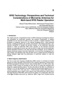
Figure 1 offers an illustration of how the

meta-frontier FF function encompasses the stochastic frontiers of the different countries. The stochastic FF cost frontiers for individual countries in the case of a single output are drawn and denoted by frontier 1, frontier 2, and frontier 3 in the figure.

A meta-frontier FF function is drawn as an envelope curve which surrounds 11

the three stochastic frontiers from below, using the pooled data over all countries.

Cost e Frontier 3 = f 3 ( x; ϕ3 )

e

d Frontier 2= f 2 ( x; ϕ2 )

Frontier 1 = f1 ( x; ϕ1 )

d meta-frontier= MF( x; ϕ * )

c c

Output Figure 1.

Meta-frontier Model

3.2.2 Technology Gaps Technical efficiency is evaluated by the extent to which a bank’s actual cost exceeds the efficient cost frontier. The measure of overall cost efficiency (OCE*) for bank i at time t in country r is formulated by the ratio of the minimum cost, evaluated by the meta-frontier cost, to the observed cost, adjusted by the corresponding random error: * it ( r )

OCE

e

=

X it ϕ *+Vit ( r )

(3-7)

Cit ( r )

Substituting (3-4) into (3-7), we obtain: OCEit* ( r ) =

e e

X itϕ *+Vit ( r )

X it ϕ( r ) +Vit ( r ) +U it ( r )

=e

−U it ( r )

×

e X itϕ * X ϕ e it ( r )

(3-8)

The first term on the right-hand side of equation (3-8) is the conventional technical efficiency relative to the stochastic frontier of country r - that is:

CEit ( r ) =

e e

X itϕ( r ) +Vit ( r )

X it ϕ( r ) +Vit ( r ) +U it ( r )

12

=e

−U it ( r )

(3-9)

which measures the extent to which a bank’s realized cost is in excess of the efficient cost frontier of country r.

It must range from zero to one, because U it is a

non-negative random variable by assumption.

The second term on the right-hand

side of equation (3-8) is the technology gap ratio (TGR), i.e.: TGRit ( r ) =

e X itϕ * X ϕ e it ( r )

(3-10)

The TGR mainly measures the degree of technology gap for country r whose currently available technology adopted by its banks is inferior to the technology available for all countries.

We assess the TGR using the ratio of the potential cost

that is defined by the meta-frontier FF function to the cost for the frontier FF function for country r holding the observed outputs and input prices constant.

It must have

a value between zero and one due to restriction (3-6). The overall cost efficiency measure of equation (3-7) can be re-written as:

OCEit* ( r ) = CEit ( r ) × TGRit ( r )

(3-11)

which must also lie between zero and one, because its components are both between zero and one.

3.2.3 Estimation Procedure The estimation procedure is divided into three steps. 1.

Obtain the maximum likelihood estimates, ϕˆ ( r ) , of ϕ (r ) in the stochastic cost frontier for country r .

2.

Get the estimate of ϕ * in the meta-frontier FF cost function, using the mathematical programming approach. Details are discussed shortly.

3.

Calculate the technical efficiency measure, the technology gap ratio, and scale

13

economies, using ϕˆ ( r ) obtained by Step 1. In line with Battese et al. (2004), there are two alternative ways to identify the best meta-frontier. One of them is based on the sum of absolute deviations of the meta-frontier values from those of the group frontiers, and the other is based on the sum of squares of the same deviations. I.

Minimum sum of absolute deviations

ϕˆ * is yielded by solving the optimization problem: T

N

min L* ≡ ∑∑ ln f ( X it , ϕˆ ( r ) ) − ln f ( X it , ϕ *)

(3-12)

s.t. ln f ( X it , ϕ *) ≤ ln f ( X it , ϕˆ (r ) )

(3-13)

t =1 i =1

Equations (3-12) and (3-13) state that the estimated meta-frontier minimizes the sum of absolute logarithms of

f ( X it , ϕˆ ( r ) ) / f ( X it , ϕ *) , which represents the

reciprocal of the radial distance between the meta-frontier and the frontier of country r .

The weights of the deviations for all banks in the sample are the same.

It is conceivable that all the deviations must be positive due to constraint (3-13). Therefore, the sign of absolute values can be removed. Thus, we can simplify the above optimization problem to the linear programming (LP) problem: min L* ≡ ∑∑ (X it ϕˆ ( r ) − X it ϕ *)

(3-14)

s.t. X it ϕ * ≤ X it ϕˆ ( r )

(3-15)

T

N

t =1 i =1

II.

Minimum sum of squares of deviations: The other approach minimizes the sum of squares of the deviations between the

meta-frontier and the frontier of the individual countries.

Here, ϕˆ * is estimated by

solving a quadratic programming (QP) problem:

min L * * ≡

∑ ∑ (X T

N

t =1 i =1

it

ϕˆ ( r ) − X it ϕ * )2 14

(3-16)

s.t. X it ϕ * ≤ X it ϕˆ ( r )

(3-17)

What is immediately apparent in equation (3-16) is that the larger the technology gap ratio of the bank is, the higher weight to the deviation is.

Standard errors of the estimators for the two meta-frontier functions can be obtained by either simulation or bootstrapping methods.

We elect the latter

procedure as the advantage of the bootstrap is that one does not need to know the underlying data generation process, unlike the Monte Carlo simulation.

The

bootstrap is frequently exploited by applied econometric research, when an analytic estimate of the standard error of an estimator is hardly calculated like the case of this paper.

It is an alternative that may provide a better finite sample approximation.

4. Data Description The main data source is from the Bankscope database spanning 1994 to 2003. We use unconsolidated accounting data for 689 banks in nine European countries, i.e., Austria, Belgium, Denmark, France, Germany, Italy, Portugal, Spain, and Switzerland. We only select those banks with at least three years of observed data. The total number of observations is 4,220. Moreover, all the nominal variables have been transformed into real terms by the consumer price index of individual countries with base year 1985.

[Insert Table 1 Here]

Three output categories can be identified: loans ( Y1 ), investments ( Y2 ), and 15

non-interest revenues ( Y3 ). three defined inputs:

On the basis of the intermediation approach, there are

physical capital ( W1 ), borrowed funds ( W2 ), and labor ( W3 ).

The price of physical capital is computed as the ratio of other non-interest expenses to fixed assets.

The price of borrowed funds is measured by the ratio of paid interest to

all funding.

As data on the number of employees are unavailable from the databank,

the price of labor is defined as the ratio of personnel expenses to total assets. Altunbas et al. (2000, 2001), Weill (2004), and others adopted the same definition. Total costs are the sum of the above three items of expenditure. Table 1 summarizes descriptive statistics and the distributions of the sample banks among countries. It can be seen from these statistics that there are substantial differences among the sample countries.

5. Empirical Results [Insert Table 2 Here]

5.1 Parameter Estimates We estimate both the FF cost function of (3-1) and the standard translog cost function for each of the nine countries using Frontier 4.1 software (Coelli, 1996). Table 2 summarizes the parameter estimates of the translog part, while the trigonometric terms are not shown to save space, but are available upon request to the authors.

Appendix 1 reports parameter estimates of the standard translog cost

function. According Table 2, more than one half of the parameter estimates of each country frontier (except for Austria) attain statistical significance at least at the 10% level of significance. The null hypothesis that the coefficients of the Fourier series are joint zero is decisively rejected in each country using the likelihood ratio test.

It

is thus concluded that the FF cost function is more appropriate than the translog form

16

in representing an average bank’s production technology and underlying cost structure. Inferences of technical efficiency and scale economies on the basis of the FF function are likely to be more reliable and reasonable than the translog form.

Evidence is found that there are seven countries having significant estimates of

η . The technical inefficiency evolves with time in most of the sample states. Five out of the seven significant η estimates are negative, showing that banks’ technical efficiencies in Austria, Belgium, France, Spain, and Switzerland deteriorate over time at an increasing rate. In other words, those banks’ actual production costs deviate from their respective country frontiers, which themselves shift over time due to the presence of technological advance.

Banks’ technical efficiencies in Denmark and

Italy improve over time, as their η estimates are positive.

Banks’ actual production

costs in the two nations move closer to their respective country frontiers. their country frontiers shift over time.

The remaining

Again,

η estimates fail to attain

statistical significance, meaning that banks’ technical efficiencies in Germany and Portugal are time invariant during the sample period.

The foregoing shows that considerable variations exist across nations not only in the coefficients, but also in the technical efficiency scores. Moreover, there are five estimates of μ that are significant at the 1% level, indicating that the corresponding five country frontiers should be modeled using a truncated normal distribution to represent the one-sided error.

Since most of the parameter estimates of σ 2 and

σ u2 /(σ u2 + σ v2 ) in the sample states achieve statistical significance, this supports the use of an error component model to fit the data.

17

There are quite a few papers in the literature, e.g., Allen and Rai (1996), Altunbas et al. (2001), and Vennet (2002) to mention a few, that attempted to estimate a unique cost frontier for all banks from distinct nations. The correctness of such a procedure depends heavily on the conditions that those banks adopt a common production technology.

Since different nations usually choose distinct political

institutions and law and tax systems and are faced with dissimilar natural endowments, bank managers of different nations tend to adopt heterogeneous production technology. This implies that the country specific cost frontiers are not necessarily the same.

In turn, the average CE score of a country operating under a type of

technology should not be compared with that of other countries operating under a different type of technology due to their evaluations failing to be on the same ground (same cost frontier). This incomparability among national frontiers can be easily resolved by relying on the meta-frontier technique, which provides extra information on TGRs.

[Insert Table 3 Here]

Table 3 uses the acronyms, SFA-POOL, MF-LP, and MF-QP, to represent three models, in which SFA-POOL is the FF cost frontier estimated by the maximum likelihood by pooling all banks of the nine countries together, and MF-LP and MF-QP are the meta-frontier FF cost functions estimated by solving the linear and quadratic mathematical programming problems using the same data. results from the standard translog counterparts.

Appendix 2 reports the

Estimating the pooled model of

SFA-POOL permits us to formally test for the differences among the group specific frontiers. A likelihood-ratio (LR) test can now be performed to test for the null 18

hypothesis that all of the countries’ FF cost frontiers are the same, i.e., the group specific frontiers are identical.

Since the value of likelihood ratio is equal to

6951.94, the hypothesis is decisively rejected even at the 1% level with degrees of freedom 368.

One is led to conclude that the group specific frontiers are

heterogeneous, i.e., banks of different countries operate under distinct types of technology.

It is noticeable that the translog results of Appendix 2 lead to the same

conclusion on the heterogeneity of group specific frontiers.

The foregoing justifies the use of the meta-frontier model.

The standard errors

attached to the estimates of MF-LP and MF-QP are obtained through bootstrapping methods.

The same applies to the translog case of Appendix 2. We randomly draw

replacements for 10000 new datasets of the same size as the original sample.

After

solving for the LP (QP) mathematical programming problems using these created datasets, we yield 10000 parameter estimates for each coefficient.

The estimated

standard error of a meta-frontier parameter is calculated as the standard deviation of the 10000 new parameter estimates.

Inspecting both the coefficient estimates and

the bootstrapped standard deviations, it is interesting to note that the coefficients of MF-LP are quite close to those of the MF-QP.

However, there are considerable

differences between the both meta-frontier coefficients and the corresponding coefficients of the SFA-POOL.

Moreover, the vast majority of the bootstrapped

standard deviations are relatively small to the corresponding coefficients.

This

implies that both MF-LP and MF-QP coefficients are quite accurately estimated and hence well representative of the meta-cost function.

The two sets of meta-frontier

parameter estimates give rise to very close estimates of the TGRs.

We therefore

arbitrarily select to show the relevant results calculated using the MF-QP estimates to 19

save space.

Appendix 2 reveals that both the coefficient estimates and the bootstrapped standard deviations have the similar feature as the FF model, among SFA-POOL, MF-LP, and MF-QP.

Nevertheless, there still exist some differences among them,

e.g., most of the bootstrapped standard deviations of the FF model are smaller than those obtained from the translog cost function.

As Gallant (1982) has shown that the FF function can approximate the true function as closely as desired in the Sobolev norm, it is the convention that the parameter estimates of the FF cost function are directly usable to compute various measures of interest without the need to check whether or not they satisfy the regularity conditions imposed by microeconomic theory.

We exploit these parameter

estimates to calculate the technical efficiency of CEit ( r ) for each nation r, based on the formula proposed by Battese and Coelli (1992), i.e., E[exp(−U it ) | ε it ] , 1 which is also built in Frontier 4.1.

Table 4 shows the average technical efficiency scores of

the banks relative to the FF cost frontiers for the nine states.

Appendix 3 presents

the same average measures relative to the translog cost frontiers.

[Insert Table 4 Here]

5.2 Cost Efficiencies and Technology Gap Ratios According to Table 4, the mean cost efficiencies of the country frontiers (CE) lie 1

Readers are suggested to refer to Battese and Coelli (1992) and Kumbhakar and Lovell (2000) for a detailed derivation. 20

in scope from 0.733 in Germany to 0.978 in Portugal during the ten-year period with an overall average value of 0.8246 and a standard deviation of 0.126.

This result

falls in the range achieved by related bank efficiency studies for West European banks, for example, Schure et al. (2004), Altunbas et al. (2001), Carbo et al. (2002), Maudos et al. (2002), and Weill (2004).

These averages show that a representative bank in

Germany is capable of cutting its current expenditure up to 27%, which is ascribable to the managerial inability to optimize costs, and still produces the same output mix. In other words, the best practice bank in Germany incurs 73% of the representative bank’s cost in providing the same output levels. The potential cost savings for an average Portuguese bank are merely 2.2%, whose actual cost is quite close to its cost frontier. Although technical inefficiency appears to be small in some countries, it is nevertheless pervasive in the banking sectors of the sample states.

As far as the TGR is concerned, its mean value ranges from about 0.51 (Denmark) to 0.62 (Belgium) with the overall mean value of roughly 0.56.

Belgian

banks are found to adopt the most advanced technology so as to offer a variety of financial services to their customers such that their cost frontier is relatively closer to the meta-cost frontier than other countries’ cost frontiers.

Belgian banks can on

average cut their frontier costs by up to 38%, if the potential technology available to all countries, the technology corresponding to the meta-frontier, is undertaken.

On

the contrary, Danish banks utilize the most inferior production process to produce financial outputs, as their country frontier lies the farthest away from the meta-frontier. The potential cost savings of an average Danish bank are as high as 49% of their frontier costs.

All cost frontiers of the countries, except one (Italy), are found to be

tangent to the meta-frontier, because these countries reach the maximum estimated values of TGR, i.e., unity. 21

Portuguese banks have the highest CE scores among all sample states and they also adopt superior production technologies, as their mean TGR (about 0.62) stands at the second highest.

Belgian banks have a similar situation, where they have both

higher mean CE and TGR scores than the respective overall averages. Conversely, German banks exhibit both lower mean CE and TGR scores than the respective overall averages.

The remaining banks in Austria, Denmark, Italy, and Spain have

higher country specific mean CE scores together with lower mean TGRs than the respective overall averages, while banks in France and Switzerland have lower average country specific mean CE scores along with higher mean TGRs than the respective overall averages.

French banks employ the most superior production

technology to provide financial services at the expense of deviating farther apart from their own cost frontier, which is found to be the closest to the meta-frontier.

[Insert Figure 2 Here]

Figure 2 shows frequency distributions of the TGRs for each country and for all countries pooled together.

It is clear to see that when combining sample states

altogether, the frequency distributions nearly form a bell shape centered at 0.5. Viewed from the angle of individual countries, the shapes look somewhat different among the countries involved. Banks in Austria, Denmark, France, Germany, Italy, Spain, and Switzerland roughly exhibit symmetrical frequency distributions of the TGRs, centered at around 0.5. Banks in Belgium and Portugal tend to have skew frequency distributions to the left.

It may be drawn that a country with an

asymmetrical distribution of TGRs is apt to have the best (Belgium and Portugal) technological achievement.

Therefore, the frequency distributions of a nation render 22

an important signal on the level of production technology adopted by that nation.

The mean values of CE* vary from around 0.40 to 0.60 with an overall mean value of 0.46.

A representative bank is able to shave up to 54% of its current

production cost for the given level of outputs.

The component CE of all countries is

on average much higher than the component TGR.

The main source of

inefficiencies stems from undertaking inferior technology, instead of managerial inefficiency.

The results suggest that the sample banks make efforts to catch up with

the potential technology available to all countries, followed by improving their managerial ability, in order to effectively reduce production costs and to be viable in the competitive market.

The adoption of advanced technology shifts the country

frontier down toward the meta-frontier. As expected, the mean cost efficiency score relative to the meta-frontier, CE*, of Portugal and Belgium stands at the first and second place, respectively, and the mean CE*s of Germany ranks last, tightly close to Switzerland and Austria. The foregoing confirms the argument that the existence of different technologies should be properly taken into account, especially when a researcher attempts to make comparisons of efficiencies in a cross-border scenario.

It is important to note that the meta-frontier model offers insightful information by subdividing the measure of CE* into measures of CE and TGR.

Informed of this

information, both bank managers and regulators could evaluate a bank’s performance more accurately, enabling them to redistribute scarce resources to where they are most productive and to enact and enforce the most appropriate policies with the hope of enhancing banks’ efficiencies and productivities and the well-being of the society as a whole.

Lacking such valuable information, managers’ and regulators’ decisions may

lead to undesirable consequences of raising the production costs and the selling price, 23

which in turn may result in smaller output quantities and/or inferior quality. Meta-cost frontier efficiency is likely to be preferable to conventional cost frontier efficiency due to its failure to impose the restriction that all countries under consideration operate under the same technology.

This facilitates researchers in

characterizing a bank’s production process and provides a common standard against which banks’ efficiencies in different countries can be meaningfully compared with one another.

[Insert Figure 3 Here]

It may be interesting to explore if the CE scores are correlated with the TGRs. This relationship provides valuable information on the potential link between production efficiency and technology achievement.

Using the sample means of CE

and TGR for the nine countries shown in Table 3, we calculate their simple correlation coefficient as 0.1055. TGR.

Figure 3 draws the nine combinations of the means CE and

This scatter diagram shows a quite weak, positive association between CE

and TGR.

One is led to infer that a higher mean value of CE is accompanied by a

higher mean value of TGR.

This implies that in a country operating under a more

advanced technology (a higher mean TGR) its banks’ realized costs tend to get close to its country frontier, resulting in a higher CE score.

On the contrary, a negative

relationship is reached by the translog cost function. The simple correlation coefficient is calculated as -0.8139. 2

[Insert Figure 4 Here]

2

Battest et al. (2004) yielded a similar negative relationship between CE and TGR, using a translog production function. 24

We next attempt to analyze the trending of the CE and the TGR during the sample period.

In order to remove random shocks from the data, the CE scores and

the TGRs are averaged across countries for each year.

Figure 4 draws these mean

values of the CE and TGRs. Both CE and TGR derived from the FF function slightly decrease with time, from around 0.85 to 0.80 and from around 0.47 up 0.60 and down to 0.53, respectively.

However, the relevant trending derived from the

translog function is dissimilar. Its mean CE grows with time, from 0.74 to 0.79, while its mean TGR exhibits a similar trend to that of the FF function, from 0.40 up to 0.50 for the first eight years and then down to 0.47 in the last year. The use of the translog function leads one to conclude that the mean value of the CE gradually improves over time, which is likely to be questionable. Appendix 3 lists the results yielded by the translog cost function model using the same dataset. Analogous to the findings of Huang and Wang (2004), the CE scores of individual countries obtained from the FF cost frontiers are higher than the corresponding CE scores obtained from the translog cost frontiers.

Recall that the

overall potential cost savings of the former are about 18% of the current expenditures (Table 4), while the latter are around 23%.

This may be attributed to the fact that the

FF function is able to fit the data more closely, because of its capability to globally approximate the underlying true function.

Although the orders of the mean TGRs of

the individual countries derived from the FF and the translog frontiers are mixed, the overall mean TGR of the FF frontier is still greater than that of the translog frontier. It is natural that the overall average value of CE* deduced from the FF frontiers exceeds that deduced from the translog frontiers.

[Insert Figure 5 Here] 25

5.3 Estimates of Scale Economies Using formula (3-2) along with the parameter estimates of the country cost frontiers and the SFA-POOL in Tables 2 and 3; we compute the measure of scale economies for all the sample banks. measures for each country.

Table 5 shows the mean values of these

The results of the scale economy estimates for the

country specific frontiers are in accordance with previous studies, such as Vennet (2002), Cavallo et al., (2001), Altunbas et al., (1996), and Allen et al., (1996). Specifically, banks in Belgium, Denmark, Italy, Spain, and Switzerland reach the optimal production scale as their measures of scale economies are quite close to unity on average.

Equivalently, their long-run average costs attain the minimum.

Banks

in Austria, France, and Germany exhibit increasing returns to scale, and these banks provide various financial products on the decreasing portion of the long-run average cost curve. As the economies of size are not exhausted, banks of these countries can further reduce their average costs by means of expanding their production scale, such as conducting mergers and acquisitions.

Conversely, Portuguese banks appear to

produce on the increasing portion of the long-run average cost curve, implying that it is beneficiary for them to shrink the production scale. By doing so, their average costs fall.

It is seen that the mean scale economy measures from the country frontier are much higher than those from the SFA-POOL.

The imposition of a common

production technology on the financial industry of different countries tends to bias the estimates of scale economies downward so that all banks of the sample states exhibit increasing returns to scale.

For the purpose of comparison, the same mean measures

of scale economies based on the translog frontier are reported in Appendix 4. There 26

are four countries, i.e., Austria, Denmark, France, and Germany, exhibiting economies of size, evaluated by the country frontiers. Banks in Belgium, Italy, Spain, and Switzerland exhibit constant returns to scale, while Portuguese banks still display diseconomies of scale.

Again, the mean measures of scale economies using the

common frontier tend to be underestimated. 3

We calculate the average scale economies across countries for each year. The mean scale economies using the FF function grow with time from 0.81 in 1994 to 0.99 in 2003.

This implies that the sample banks on average keep adjusting their

production scale toward the optimal scale. 4 Conversely, the mean scale economy estimates from the translog cost function do not change very much.

They are around

0.97 during the sample period.

6. Concluding Remarks This paper has examined the performance of the commercial banks across nine European countries spanning 1994-2003 in terms of cost efficiency and technology gap ratios. A Fourier flexible cost frontier and the meta-cost frontier are particularly applied.

The adoption of the newly developed meta-cost function successfully

solves the incomparability problem, when one attempts to compare the technical efficiency scores for banks across countries due to the fact that those banks potentially operate under different technologies.

The existence of multiple technologies

3 Ivaldi et al. (1996) applied both the Fourier and the translog cost functions to describe the technology of French farmers. Their estimation results and statistical tests tend to favor the Fourier specification and show that the Fourier cost function is able to represent a broader range of technological structures than the translog one. 4 As pointed out by Altunbas et al. (1993), scale economies typically range between 5% and 7%, implying that a 100% increase in the level of outputs will lead to about a 93% to 95% increase in total costs. 27

justifies the utilization of the meta-cost frontier, under which the relevant technical efficiencies are evaluated against the common cost frontier.

The mean CE scores for the sample countries are detected to fall into the range of the prior works and are positively correlated with the TGRs.

This implies that a

relatively technically efficient bank is usually technologically efficient and vice versa. Most of the average TGRs for the sample countries are much less than those of the average CE scores.

The results suggest that there are many banks operating off the

meta-cost frontier.

These banks need to catch up with the potential technology

accessible to all countries in order to be competitively viable. Evidence is found that there exists substantial variability in the technology gap ratios for banks in the nine sample countries.

Some banks appear to adopt inferior technologies to produce an

array of financial services.

As for scale economies, mixed results are reached if measured under the country specific frontiers. However, when a common production technology is imposed, economies of size prevail over all the sample states.

28

References Agarwal, R. and Audretsch, D.B. (2001) Does entry size matter? The impact of the life cycle and technology on firm survival, Journal of Industrial Economics, 49, 21-43. Aigner, D.J. C.A.K. Lovell and P. Schmidt (1977), Formulation and estimation of stochastic frontier production function models, Journal of Econometrics, 6, 21-37. Alhadeff, D.A. and C.P. Alhadeff (1964), Growth of large banks 1930-1960, Review of Economics and Statistics, 46, 356-363. Allen, L. and A. Rai, (1996) “Operational Efficiency in Banking: An International Comparison”, Journal of Banking and Finance, 20, 655-72. Altunbas, Y., L. Evans, and P. Molyneux (2001), Bank ownership and efficiency, Journal of Money, Credit and Banking, 33, 926-954. Altunbas, Y., E.P.M. Gardener, P. Molyneux and B. Moore, (2001), Efficiency in European Banking, European Economic Review, 45(10), 1931-1955. Altunbas, Y., M.H. Liu, P. Molyneux, and R. Seth (2000), Efficiency and risk in Japanese banking, Journal of Banking and Finance, 24, 1605-1628. Audretsch, D.B. and J.A. Elston (2006), Can institutional change impact high-technology firm growth? evidence from Germany’s Neuer Markt, Journal of Productivity Analysis, 25, 9-23. Baldini, D., Landi, A., 1990. Economie di scala e complementarieta' di costo nell'industria bancaria italiana, L'Industria 1, 25-45. Barnes, P., Dodds, C., 1983. The structure and performance of the UK building society industry 1970-78. Journal of Business, Finance and Accounting 10, 37-56. Battese, G.E. and T.J. Coelli (1988), Prediction of firm-level technical efficiencies with a generalized frontier production function and panel data, Journal of Econometrics, 38, 387-399. Battese, G.E. and T.J. Coelli (1992), Frontier production functions, technical efficiency and panel data: With application to paddy farmers in India, Journal of Productivity Analysis, 3, 153-169. Battese, G.E., and T.J. Coelli (1995), A model for technical inefficiency effects in a stochastic frontier production function for panel data, Empirical Economics, 20, 325-332. Battest, G.E., D.S. Prasada Rao (2002), Technology gap, efficiency and a stochastic metafrontier function, International Journal of Business and Economics, 1, 1-7. Battest, G.E., D.S. Prasada Rao, and C.J. O’Donnell (2004), A metafrontier production function for estimation of technical efficiencies and technology gaps for firms 29

operating under different technologies, Journal of Productivity Analysis, 21, 91-103. Berger, A.N. and R. DeYoung (1997), Problem loans and cost efficiency in commercial banks, Journal of Banking and Finance, 21, 849-870. Berger, A.N., J.H. Leusner, and J.J. Mingo (1997), The efficiency of bank branches, Journal of Monetary Economics, 40, 141-162. Berger, A.N. and L.J. Mester (1997), Inside the black box: What explains differences in the efficiencies of financial institutions? Journal of Banking and Finance, 21, 895-947. Berger, A.N. and T.H. Hannan (1998), The efficiency cost of market power in the banking industry: A test of the quiet life and related hypotheses, Review of Economics and Statistics, 81, 454-465. Chalfant, J.A. and A.R. Gallant (1985), Estimating substitution elasticities with the Fourier cost function: Some Monte Carlo results, Journal of Econometrics, 28, 205-222. Chaffai, M.E., M. Dietsch and A. Lozano-Vivas, (2001) “Technological and Environmental Differences in the European Banking Industries”, Journal of Financial Services Research, 19(2/3), 147-162. Charnes, A., W.W. Cooper, and E. Rhodes (1981), Evaluating program and managerial efficiency: An application of data envelopment analysis to program follow through, Management Science, 27, 668-697. Congliani, C., DeBonis, R., Motta, G., Parigi, G., 1991. Economie di scala e di diversi"cazione nel sistema bancario. Banca d'Italia, Temi di discussione 150. Cooper, J.C.B., 1980. Economies of scale in the UK building society industry. Investment Analysis 55, 31-36. Cornwell, C., P. Schmidt, and R.C. Sickles (1990), Production frontiers with cross-sectional and time-series variation in efficiency levels, Journal of Econometrics, 46, 185-200. Cossutta, D., Di Battista, M.L., Giannini, C., Urga, G., 1988. Processo produttivo e struttura dei costi nell'industria bancaria italiana. In: Cesarini, F., Grillo, M., Monti, M., Onado, M. (Eds.),Banca e Mercato a cura. Il Mulino, Bologna DeYoung, R., I. Hasan, and B. Kirchhoff (1998), The impact of out-of-state entry on the efficiency of local banks, Journal of Economics and Business, 50, 191-203. De Bandt, O. and E.P. Davis (1999), A cross-country comparison of market structure in European banking, European Central Bank Working Paper No. 7, Frankfurt: European Central Bank. Dietsch, M., 1988. Economies d'echelle et economies d'envergure dans les banques de depots franc7 aises. Mimeo., Institut d'Etudes Politiques de Strasbourg. 30

Dietsch, M., 1993. Economies of scale and scope in the French commercial bank industries. Journal of Productivity Analysis 1, Dietsch, M. and Lozano-Vivas, A., (2000) “How the Environment Determines Banking Efficiency: A Comparison between French and Spanish Industries”, Journal of Banking and Finance, 24, 985-1004. Drake, L., Howcroft, B., 1994. Relative efficiency in the branch network of the UK bank: An empirical study. Omega 22 (1), 83-96. Elbadawi, I., A.R. Gallant and G. Souza (1983), An elasticity can be estimated consistently without a priori knowledge of functional form, Econometrics 51, 1731-1753. Evans, D.S. (1987), Tests of alternative theories of firm growth, Journal of Political Economy, 95, 657-674. Fecher, F. and P. Pestieau, (1993) “Efficiency and Competition in O.E.C.D. Financial Services. In H.O. Fried, C.A.K. Lovell and S.S. Schmidt, eds. The Measurement of Productive Efficiency: Techniques and Applications, Oxford University Press, U.K., 374-385. Gallant, A. R. (1982), Unbiased determination of production technologies, Journal of Econometrics, 20, 285-323 Gibrat, R. (1931), Les Inegalites Economiques, Paris, Recueil Sirey. Goddard, J.A., D.G. McKillop, and J.O.S. Wilson (2002), The growth of US credit unions, Journal of Banking and Finance, 26, 2327-2356. Gough, T.J., 1979. Building society mergers and size efficiency relationship. Applied Economics 11,185-194. Grigorian, D.A and V. Manole, (2002) “Determinants of Commercial Bank Performance in Transition: An Application of Data Envelopment Analysis”, World Bank Policy Research Working Paper, 2850, June. Hardwick, P., 1989. Economies of scale in building societies. Applied Economics 21, 1291-1304. Hart, P.E. and N. Oulton (1999), Gibrat, Galton and job creation, International Journal of the Economics of Business, 6, 149-164. Huang, Tai-Hsin and Mei-Hui Wang (2001), Estimating scale and scope economies with Fourier flexible functional form—Evidence from Taiwan’s banking industry, Australian Economic Papers, 40, 213-231. Huang, Tai-Hsin and Mei-Hui Wang (2003), Estimation of technical and allocative inefficiency using the Fourier flexible cost frontiers for Taiwan’s banking industry, The Manchester School, 71, 341-362. Huang, Tai-Hsin and Mei-Hui Wang (2004), Comparisons of economic inefficiency between output and input measures of technical inefficiency using the Fourier 31

flexible cost frontiers, Journal of Productivity Analysis, 22, 123-142. Ivaldi, M., N. Ladoux, H. Ossard, and M. Simini (1996), Comparing Fourier and translog specifications of multiproduct technology: Evidence from an incomplete panel of French farmers, Journal of Applied Econometrics, 11, 649-667. Juan Fernández de Guevara, Joaquín Maudosand and Francisco Pérez(2005), Market Power in European Banking Sectors , Journal of Financial Services Research,109-137 Jaap W. B. Bos and Heiko Schmiedel (2006), Is there a single frontier in a single European banking market? , European Central Bank Working Paper No. 701, Frankfurt: European Central Bank. Kumbhakar, S.C. (1987), The specification of technical and allocative inefficiency in stochastic production and profit frontiers, Journal of Econometrics, 34-335-348. Kumbhakar, S.C. (1990), Production frontiers, panel data, and time-varying technical inefficiency, Journal of Econometrics, 46, 201-212. Lang, G., Welzel, P., 1996. Efficiency and technical progress in banking: Empirical results for a panel of German cooperative banks. Journal of Banking and Finance 20, 1003-1023. Levy-Garboua, L., Renard, F., 1977. Une etude statistique de la rentabiliteH des banques en France en 1974. Cahiers Economiques et Monetaires, Vol. 5. Lozano-Vivas, A., J.T. Pastor and I. Hasan, (2001),European Bank Performance beyond Country Borders: What really matters?, European Finance Review, 5(1/2), 141-165. McKillop, D.G., Glass, J.C., 1994. A cost model of building societies as produces of mortgages and other "nancial products. Journal of Business, Finance and Accounting 217, 1031-1046. Meeusen, W., and J. Van Den Broeck (1977), Efficiency estimation from Cobb-Douglas production functions with composed error, International Economic Review, 18, 435-444. Mitchell, K. and N.M. Onvural (1996), Economies of scale and scope at large commercial banks: Evidence from the Fourier flexible function form, Journal of Money, Credit, and Banking, 28, 178-199. Molyneux, P., Y. Altunbas and E. Gardener, (1997), Efficiency in European Banking, John Wiley & Sons, West Sussex, UK. Pitt, M., and L.F. Lee (1981), The measurement and sources of technical inefficiency in the Indonesian weaving industry, Journal of Development Economics, 9, 43-64. Rhoades, S.A. and A.J. Yeats (1974), Growth, consolidation and Mergers in banking, Journal of Finance, 29, 1397-1405. 32

Ruthenberg, D. and R. Elias, (1996) ,Cost Efficiencies and Interest Margins in a Unified European Banking Market,, Journal of Economics and Business, 48, 231-249. Saunders, Anthony, and IngoWalter (1994). Universal Banking in the United States? Oxford,Oxford University Press. Schmidt, P., and R.C. Sickles (1984), Production frontiers and panel data, Journal of Business and Economic Statistics, 2, 367-374. Scholtens, Bert (2000),Competition, Growth and Performance in the Banking Industry,Department of Finance Working Paper. Netherlands: University of Groningen. Shaffer, S. (2001), Banking conduct before the European single banking license: A cross country comparison, North American Journal of Economics and Finance, 12, 79-104. Sheldon, G., (1999) ,Costs, Competitiveness and the Changing Structure of European Banking, Working Paper, Fondation Banque de France pour la Recherche. Singh, A. and G. Whittington (1975), Growth, Profitability and Valuation, Cambridge, Cambridge University Press. Weill, L. (2004), Measuring cost efficiency in European banking: A comparison of frontier techniques, Journal of Productivity Analysis, 21, 133-152.

33

Table 1 : Descriptive statistics of dataset - country average. Variable Total number of banks Total number of observations

Total cost*

Austria

Belgium

Denmark

France

Germany

Italy

Portugal

Spain

Switzerland

21

30

48

155

141

120

22

58

94

137

187

339

904

858

762

134

362

537

342.0152

1167.265

173.9057

624.3617

601.6766

441.7648

221.4476

314.2474

498.0184

(738.4505) (3675.096 )

(525.9168)

(2021.889)

(2524.793) (1118.801 ) ( 298.1051)

(770.0886) (2430.416)

Outputs Total loans(Y1)*

Total investments(Y2)*

Non-interest revenue(Y3)*

5752.409

7225.775

2476.789

6359.059

8570.908

5146.058

2173.042

(11817.73)

(16277.07)

(7901.521)

(20593.39)

1176.849

3416.71

1063.206

2463.28

(2678.022)

(7215.941)

(3947.685)

(9506.188)

47.04695

521.167

39.99939

129.5784

121.7847

97.76005

(75.09649)

(1150.097)

(140.0078)

(528.0417)

(615.476)

(227.9904)

0.0873138

5.33596

1.549729

4.018975

2.956362

1.388497

1.030388

(0.767428)

(6.232226)

(2.729975)

(5.790903)

(4.257878)

(2.129666)

(0.997869)

0.032372

0.076208

0.028996

0.048651

0.04636

0.041598

0.061672

(0.009282) (0.122387 )

(0.010293)

(0.060233)

(0.128257)

(0.028925)

0.013804

0.017592

3993.13

7100.584

(35254.7) (12781.83 ) (2897.741 ) ( 9237.666) (34459.6 ) 2853.299

1278.187

506.1777

1280.924

2393.666

(15127.12) (3135.284 ) (750.3299 ) (4187.907 ) (14168.81) 110.3945

59.68363

168.7931

(219.4341) (133.6222 ) (767.7259 )

Input prices Price of physical capital(W1)

Price of borrowed funds(W2)

Price of labor(W3)

0.014011

0.022089

0.020038

0.017111

(0.008282)

(0.035197)

(0.008776)

(0.0124)

Note: *: All values are in real millions dollars, with base year 1985.

34

2.344001

(1.492468) (4.935645 ) 0.044517

0.031389

(0.064276) (0.082162 ) (0.017107 ) 0.011653

(0.009764) (0.0 10026) ( 0.006026)

Standard deviations are in parentheses.

0.992091

0.015757

0.018001

(0.012327) (0.017082 )

Table 2 : Cost Fourier Flexible Stochastic Frontier Models for European Banks Variable

constant ln Y1 ln Y2 ln Y3 lnW2

Austria

Belgium 9.0943 **

(0.9301)

(8.0320)

-0.6644

0.4017

-0.5148

(1.3155)

(-0.2782)

(0.4292)

0.1616

(-0.1637)

0.8359

0.1206

(1.1572)

(0.2827)

1.1995 **

0.2723

0.0552 (0.0869)

ln Y2 ln Y2 ln Y3 ln Y3 ln Y1 ln Y2

1.4838 ***

(1.1601)

(0.4676)

ln Y1 ln Y1

13.8479 *

(4.1115)

(0.5347)

lnW3

0.5749

Denmark

0.0015

0.4076 *** (0.0898) 0.6567 *** (0.0765) 0.0531 *** (0.0221) -0.0245 **

0.6744 *** (0.2468) -1.0535 * (0.6536) 0.3308 *** (0.1001) 0.4277 *** (0.0743) 0.1716 *** (0.0357) 0.0442 **

France

Germany

0.5857 (0.9474) 0.6323 *** (0.2783) 0.5144 *** (0.0745) 0.1533 ** (0.0630) 0.4370 *** (0.0326) 0.4026 *** (0.0254) 0.0666 *** (0.0174) 0.0229 ***

-3.8755 *** ( 0.9582) -0.0966 (0.4885) 3.4704 *** ( 0.5241) 0.1539 (0.5325) 0.9407 *** ( 0.1583) 0.1219 (0.1235) 0.0784 * (0.0421) -0.2093 ***

Italy

Portugal

1.0755 *** (0.3997) 0.5724 *** (0.1621) 0.5321 *** (0.1138 ) 0.1751 * (0.0908) 0.2183 *** (0.0496) 0.7208 *** (0.0417) 0.0764 *** (0.0137) 0.0485 ***

Spain

Switzerland

1.2045

3.0265

(0.9608)

( 5.6858 )

0.2565 (0.4765) 0.7589

0.9787 *** ( 0.4000 ) 0.5335 ***

2.6850 * (1.4955 ) 0.7253 * ( 0.4274 ) -0.0781

(0.5693)

( 0.2075 )

( 0.2814 )

0.2918

0.0804

-0.0795

(0.5358)

( 0.5205 )

( 0.2147 )

-0.5121

-0.0581

(0.4711)

(0.0890 )

0.7608 * (0.4132) 0.0977 ** ( 0.0506) 0.0529

0.9189 *** ( 0.0777 ) 0.0440 (0.0329 ) 0.0391 **

0.1676 ** (0.0862 ) 0.7614 *** (0.0795 ) 0.0558 *** (0.0254 ) 0.0955 ***

(0.1101)

(0.0128)

(0.0209)

(0.0065)

(0.0431)

(0.0126)

(0.0613)

(0.0184 )

( 0.0229 )

-0.1367

-0.0238

-0.1578

0.0025

0.0338

-0.0048

-0.0824

-0.0557

0.0144

(0.1757)

(0.0325)

(0.1273)

(0.0080)

(0.0548)

(0.0143)

(0.0736)

( 0.0927 )

(0.0187 )

-0.0234 (0.0849)

-0.0862 *** (0.0225)

-0.1631 *** (0.0210)

-0.1050 *** (0.0056)

-0.1066 *** (0.0227)

Note: Standard errors are given in parentheses. ***, ** , and * denote statistical significance at the 1%, 5%, and 10 % levels, respectively.

35

-0.1174 *** (0.0082)

-0.1531 *** (0.0419)

-0.1225 *** ( 0.0162 )

-0.1119 *** (0.0256 )

Table 2 : Cost Fourier Flexible Stochastic Frontier Models for European Banks (cont.) Variable

ln Y1 ln Y3 ln Y2 ln Y3 ln W2 ln W2

Austria

Belgium 0.0024

0. 0114

-0.0058

(0.1009)

(0.0417)

(0.0317)

-0.0175

-0.0321

0.0374

(0.0856)

(0.0334)

(0.0257)

-0.0519 (0.0817)

ln W2 ln W3

0.0563 (0.1539)

ln W3 ln W3

0.0018 (0.0937)

ln W2 ln Y1

-0.0103 (0.1357)

ln W2 ln Y2

-0.1102 (0.1159)

ln W2 ln Y3

0.1527 * (0.0913)

ln W3 ln Y1

-0.0232 (0.1530)

ln W3 ln Y2

Denmark

0.0706 (0.0934)

0.1298 *** (0.0079) -0.2796 *** (0.0129) 0.1596 *** (0.0065) -0.0830 *** (0.0175) -0.0272 *** (0.0109) 0.0976 *** (0.0206) 0.1083 *** (0.0120) 0.0489 *** (0.0084)

0.0979 *** (0.0141) -0.1998 *** (0.0218) 0.0865 *** (0.0104) -0.0195 (0.0189) 0.0370 ** (0.0169) -0.0113 (0.0201) 0.0287 * (0.0166) -0.0353 ** (0.0161)

France

Germany

-0.0310 *** (0.0051) 0.0221 *** (0.0040) 0.0764 *** (0.0032) -0.1250 *** (0.0046) 0.0542 *** (0.0030) 0.0175 *** (0.0066) 0.0164 *** (0.0040) -0.0234 *** (0.0054) 0.0106 * (0.0059) -0.0235 *** (0.0036)

0.0270 (0.0177) 0.0211 (0.0161) -0.0397 ** (0.0192) 0.0831 *** (0.0318) -0.0050 (0.0164) -0.0400 * (0.0227) 0.1453 *** (0.0192) -0.0295 ** (0.0147) 0.0507 *** (0.0187 ) -0.1394 *** (0.0153)

Note: Standard errors are given in parentheses. ***, ** , and * denote statistical significance at the 1%, 5%, and 10 % levels, respectively.

36

Italy

Portugal

-0.0209 *** (0.0074) -0.0122 * (0.0064) 0.0579 *** (0.0068) -0.1189 *** (0.0105) 0.0788 *** (0.0062) 0.0208 ** (0.0084) 0.0183 *** (0.0071) -0.0316 *** (0.0092) 0.0197 *** (0.0069) -0.0241 *** (0.0058)

Spain

Switzerland

-0.0224

-0.0511

-0.0170

(0.0452)

(0.0390 )

(0.0211 )

0.0405 (0.0328) 0.0826 ** (0.0446) -0.2882 *** (0.0553) 0.0926 *** (0.0306) 0.0264 (0.0549) 0.0682 ** (0.0370) -0.0216 (0.0346) -0.0477

0.0329 * (0.0197 ) 0.0578 *** (0.0126 ) -0.1186 *** (0.0160 ) 0.0642 *** (0.0083 ) 0.1310 ***

-0.0017 (0.0170 ) 0.1047 *** (0.0122 ) -0.2122 *** ( 0.0212 ) 0.1130 *** (0.0113 ) 0.0252

(0.0181 )

(0.0209 )

-0.0148

-0.0134

( 0.0106 ) -0.0867 *** (0.0161 ) -0.1002 ***

(0.0140 ) 0.0037 (0.0184 ) -0.0144

(0.0404)

(0.0176 )

(0.0198 )

0.0201

0.0054

0.0160

(0.0318)

(0.0085 )

(0.0136 )

Table 2 : Cost Fourier Flexible Stochastic Frontier Models for European Banks (cont.) Variable

ln W3 ln Y3

Austria

Belgium -0.1643 (0.1115)

T

-0.2067 * (0.1144)

T2

0.0049 (0.0069)

T ln W2 T ln W3 T ln Y1

-0.0460 *

T ln Y3 σ2

-0.0084

0.0287

0.0071

(0.0222)

(0.0209)

(0.0101)

-0.0016 * (0.0009) -0.0007

-0.0026 *** (0.0008) -0.0073 *

0.0016

0.0026

(0.0226)

(0.0039)

(0.0034)

0.0188 *** (0.0053) -0.0095 ***

-0.0004 (0.0043) -0.0004

(0.0250)

(0.0033)

(0.0029)

-0.0096

-0.0088

0.0018

(0.0234)

(0.0073)

(0.0050)

0.1758 ***

0.8983 *** (0.0444)

0.0104 ** (0.0050)

0.0269

0.0037

Germany

(0.0166)

(0.0041)

0.0159

France

(0.0152)

(0.0042)

(0.0539)

σ u2 /(σ u2 + σ v2 )

0.0166

(0.0231)

(0.0217)

T ln Y2

-0.1501 ***

Denmark

0.1458 (0.2010) 0.9874 *** (0.0175)

0.0079 *** (0.0021) 0.7318 *** (0.0646)

0.0007 (0.0006) -0.0037 * (0.0019) 0.0047 *** (0.0016) -0.0032 * (0.0019) 0.0046 *** (0.0011) -0.0054 *** (0.0018) 0.0348 *** (0.0027) 0.8441 *** (0.0143)

0.0527 *** (0.0136) -0.1124 *** (0.0354) 0.0042 ** (0.0022) -0.0258 *** (0.0073)

Portugal

0.0046 (0.0071) 0.0370 *** (0.0152) 0.0012 * (0.0007) 0.0047

-0.0380 * (0.0226) -0.1537 * (0.0880) -0.0045 * (0.0026) -0.0262 **

Spain

Switzerland

0.0685 *** (0.0152 ) -0.0436 * (0.0265 ) -0.0017 (0.0013 ) -0.0180 ***

-0.0017 ( 0.0176 ) -0.0003 (0.0200 ) -0.0022 * (0.0012 ) 0.0022

(0.0036)

(0.0133)

-0.0003

-0.0174

(0.0031)

(0.0134)

-0.0011

-0.0010

(0.0055)

(0.0032)

(0.0135)

-0.0016

-0.0030

0.0041

0.0008

-0.0019

(0.0050)

(0.0021)

(0.0120)

(0.0030 )

( 0.0039 )

0.0021

0.0103

(0.0028)

(0.0092)

0.0227 *** (0.0062) 0.0224 ***

-0.0213 *** (0.0043) 1.1830 *** (0.0217) 0.8561 *** (0.0026)

Note: Standard errors are given in parentheses. ***, ** , and * denote statistical significance at the 1%, 5%, and 10 % levels, respectively.

37

Italy

0.0354 *** (0.0051) 0.8096 *** (0.0270)

0.0062 *** (0.0009) 0.0158 (0.0254)

(0.0062 ) 0.0216 *** (0.0047 ) 0.0161 *** ( 0.0057 )

-0.0119 *** (0.0055 ) 0.0812 *** (0.0246 ) 0.9024 *** (0.0333 )

(0.0056 ) -0.0143 *** (0.0053 ) -0.0131 *** (0.0050 )

0.0093 ** (0.0041 ) 0.0549 *** ( 0.0048 ) 0.8153 *** (0.0276 )

Table 2 : Cost Fourier Flexible Stochastic Frontier Models for European Banks (cont.) Variable

μ η

Austria

Belgium

Denmark

0.0775

-0.7589

0.0446

(0.6466)

(1.3246)

(0.0348)

-0.1849 ** (0.0857)

-0.1353 *** (0.0222)

0.0922 *** (0.0226)

France

Germany

0.3430 *** (0.0331) -0.0507 *** (0.0087)

Note: Standard errors are given in parenthesis and *** denotes statistical significance at the 1%, ** at the 5% and * at the 10 %

38

-2.0128 *** (0.6255) 0.0250 (0.0201)

Italy

Portugal

-0.3387 *** (0.0634) 0.1061 *** (0.0162)

-0.0198 (0.0504) 0.3392 (0.2667)

Spain

Switzerland

-0.5414 *** ( 0.1322 ) -0.0687 * (0.0396 )

0.4230 *** (0.0885 ) -0.1162 *** ( 0.0176 )

Table 2 : Cost Fourier Flexible Stochastic Frontier Models for European Banks (cont.) Variable

cos z1 sin z1

Austria

Belgium 0.1869

-0.0772

(0.5561)

(0.1476)

-0.5155 ** (0.2608)

cos z2

0.0707 (0.6141)

sin z2 cos z3 sin z3

-0.5867 **

sin(2 z1 ) cos(2 z2 )

1.0800 *** (0.1603) 0.2238 ***

Germany

Italy

Portugal

Spain

Switzerland

0.1585

-0.6280

-0.0674

-0.0811

0.0009

0.3013

(0.3029)

(0.1700)

(0.4358)

(0.1565)

(0.1529)

(0.2742 )

( 0.4096)

0.3383

-0.0253

(0.2425)

(0.0478)

-0.0097

0.1954 **

1.2956 *** (0.3787) 3.9681 ***

0.1164 *

-0.0592

0.7672 ***

(0.0614)

(0.1142)

(0.2590 )

0.1835

-0.0157

0.1058

-0.2545 * ( 0.1538 ) -0.3544 *

(0.2443)

(0.0927)

(0.6565)

(0.1535)

(0.5177)

(0.2559 )

(0.2165 )

-0.1694

-0.0147

0.4100

0.0604

0.0502

0.0382

0.1388

(0.0728)

(0.2252)

(0.0542)

(0.3753)

(0.0598)

(0.1620)

(0.1776 )

(0.1401 )

0.2406

0.1179

8.8702

0.0794

-0.6189

0.1217

0.3922

2.8359

-0.1619

(0.5426)

(0.1496)

(7.4685)

(0.0693)

(0.5586)

(0.0900)

(0.5085)

(5.0113 )

(0.2135 )

8.1484

0.0446

-0.2994

-0.0998

0.0574

3.3778

0.0003

(5.2269)

(0.0353)

(0.2815)

(0.0624)

(0.0671)

(4.3014 )

(0.0999 )

-0.0403

-0.0314

-0.3371

0.1370

0.1767 *** (0.0607) 0.1052 **

0.0368

-0.0574 **

0.1117 **

0.1281 ***

-0.0287

(0.1713)

(0.0451)

(0.0446)

(0.0284)

(0.0917)

(0.0327)

(0.0580)

0.0533

0.0724

0.0594

-0.0166

0.1395

-0.0124

0.0206

(0.1599)

(0.0550)

(0.0524)

(0.0250)

(0.0912)

(0.0250)

(0.0579)

(0.0509 )

(0.0705 )

0.0107

-0.0197

-0.0074

0.0095

(0.0257)

(0.1400)

(0.0473 )

( 0.0632 )

0.0007

0.1478

0.0358

(0.0210)

(0.107 6)

(0.0321 )

-0.1748 (0.1515)

sin(2 z2 )

(0.0656)

-0.8106 ***

France

(0.2216)

(0.2118)

cos(2 z1 )

-0.1911 ***

Denmark

-0.1841 (0.1473)

0.2389 *** (0.0440) -0.1224 *** (0.0333)

0.0638 *

-0.0646 ***

(0.0330)

(0.0150)

-0.0178

0.0169

(0.0402)

(0.0195)

Note: Standard errors are given in parenthesis and *** denotes statistical significance at the 1%, ** at the 5% and * at the 10 %

39

0.6885 *** (0.1054) -0.3427 *** (0.1094)

(0.0399 ) -0.1498 ***

( 0.0830 ) -0.0102

0.1296 *** ( 0.0483 )

Table 2 : Cost Fourier Flexible Stochastic Frontier Models for European Banks (cont.) Variable

cos(2 z3 ) sin(2 z3 ) cos( z1 z2 ) sin( z1 z2 ) cos( z1 z3 ) sin( z1 z3 )

Austria

Belgium

Germany

0.0586 ***

-0.0974

(0.0982)

(0.0677)

(0.5884)

(0.0171)

0.1299

0.0261

1.4091

0.0097

(0.0874)

(0.0580)

(1.3114)

(0.0172)

0.2354

0.0714

-0.1057

(0.1901)

(0.0685)

(0.0686)

(0.0233)

-0.0229

0.0271

-0.1843

-0.2137 ***

0.1756 ***

-0.0023

(0.0607)

(0.0170)

(0.1434)

(0.6209 )

(0.0363 )

0.0218

0.0582

0.6160

(0.0218)

(0.0458)

(0.8869 )

(0.0521 )

0.0116

-0.0450

0.0241

-0.0582

(0.0366)

(0.0926)

( 0.0479 )

(0.0909 )

0.0283

-0.0871

0.0659

-0.1266

(0.0309)

(0.1382)

(0.0593 )

(0.1058 )

-0.1917 * (0.1182) -0.2173 * (0.1211) 0.6344 *** (0.1355)

0.1200

-0.1192

-0.2388

-0.0296

-0.0782

(0.1663)

(0.0904)

(0.2006)

(0.0206)

(0.0688)

-0.0190

0.2228 (0.1625)

(0.0843) 0.1256 * (0.0693) 0.4529 *** (0.0912)

-0.0237

Switzerland

-0.7181

(0.0250)

-0.3964 ***

Spain

0.1863

(0.0538)

-0.0849

Portugal

-0.0193

(0.0785)

-0.5855 ***

Italy

0.0651

(0.2522)

(0.1676)

sin( z2 z3 )

-1.5837 ***

France

-0.0805

(0.1331)

cos( z2 z3 )

Denmark

-0.1872 **

-0.0993

-0.6199 ***

0.1038

(0.0244)

(0.1026)

-0.0284

-0.0634

(0.0273)

(0.1049)

(0.1461 )

(0.0736 )

-0.0519

0.1122

0.0951

(0.2377 ) -0.5008 ***

(0.0664 ) -0.1117

(0.1481)

(0.0216)

0.0707

0.0016

(0.1982)

(0.0180)

(0.0739)

(0.0226)

(0.0923)

(0.1411 )

(0.0647 )

-0.0721

-0.0165

0.0468

0.0087

-0.0814

0.1000

-0.0281

(0.1439)

(0.0189)

(0.0959)

(0.0243)

(0.1210)

Note: Standard errors are given in parenthesis and *** denotes statistical significance at the 1%, ** at the 5% and * at the 10 %

40

(0.0908)

0.0455 *

0.1222 **

-0.2117 ***

0.0372 *

(0.1275 )

(0.0461 )

Table 3: Maximum-likelihood estimates of the FF stochastic frontier using pooled data, together with the parameter estimates of the meta-frontier FF cost functions. Variable

constant ln Y1 ln Y2 ln Y3 lnW2 lnW3 ln Y1 ln Y1 ln Y2 ln Y2 ln Y3 ln Y3 ln Y1 ln Y2 ln Y1 ln Y3

SFA-POOL

MF-LP

MF-QP

1.8187 (0.9165)

0.5693 (0.4577)

0.4966 (0.4919)

0.0476 (0.3893)

1.0026 (0.1539)

1.1766 (0.1694)

0.4733 (0.1609)

0.7445 (0.1063)

0.2587 (0.1021)

-0.0650 (0.0852)

-0.6682 (0.1226)

-0.2609 (0.0922)

0.3110 (0.0417)

-0.2742 (0.1971)

0.1699 (0.1581)

0.5016 (0.0373)

0.8511 (0.1335)

0.5573 (0.1103)

0.0583 (0.0284)

-0.0616 (0.0166)

-0.0743 (0.0166)

0.0092 (0.0152)

-0.0241 (0.0102)

-0.0032 (0.0093)

0.0117 (0.0131)

-0.1096 (0.0165)

-0.0184 (0.0245)

-0.0913 (0.0084)

-0.1052 (0.0181)

-0.0540 (0.0227)

0.0418 (0.0088)

0.1909 (0.0195)

0.1120 (0.0184)

0.0271 (0.0077)

0.1074 (0.0195)

0.0467 (0.0186)

ln Y2 ln Y3 ln W2 ln W2 ln W2 ln W3 ln W3 ln W3 ln W2 ln Y1

0.0239 (0.0054)

-0.1509 (0.0282)

-0.0861 (0.0205)

-0.0733 (0.0087)

0.2017 (0.0334)

0.1154 (0.0256)

0.0489 (0.0048)

-0.0816 (0.0147)

-0.0419 (0.0130)

0.0490 (0.0083)

0.1561 (0.0331)

0.0767 (0.0332)

ln W2 ln Y2

0.0395 (0.0057)

0.1787 (0.0303)

0.1362 (0.0228)

ln W2 ln Y3

-0.0744 (0.0065)

-0.2516 (0.0274)

-0.1398 (0.0218)

ln W3 ln Y1

-0.0361 (0.0079)

-0.1577 (0.0212)

-0.0758 (0.0255)

ln W3 ln Y2

-0.0477 (0.0053)

-0.1138 (0.0200)

-0.1122 (0.0169)

ln W3 ln Y3

0.1012 (0.0059)

0.2239 (0.0198)

0.1636 (0.0157)

T

-0.0833 (0.0123)

-0.0567 (0.0323)

-0.0232 (0.0361)

T2

0.0051 (0.0007)

-0.0021 (0.0016)

-0.0057 (0.0022)

T ln W2

-0.0197 (0.0026)

-0.0429 (0.0099)

-0.0387 (0.0076)

T ln W3

0.0169 (0.0021)

0.0344 (0.0069)

0.0300 (0.0058)

T ln Y1

0.0100 (0.0021)

0.0158 (0.0049)

0.0255 (0.0052)

T ln Y2

0.0047 (0.0017)

0.0073 (0.0049)

0.0004 (0.0051)

T ln Y3

-0.0084 (0.0018)

-0.0145 (0.0043)

-0.0196 (0.0041)

cos z1

-0.3843 (0.4196)

0.1198 (0.0627)

0.2762 (0.0777)

sin z1

0.3978 (0.1629)

-0.0638 (0.0811)

-0.1415 (0.0897)

cos z2

0.2406 (0.2436)

0.0385 (0.0450)

-0.0546 (0.0532)

sin z2

-0.0112 (0.1752)

-0.3215 (0.0665)

-0.2875 (0.0740)

41

Table 3: Maximum-likelihood estimates of the FF stochastic frontier using pooled data, together with the parameter estimates of the meta-frontier FF cost functions.(cont.) Variable

SFA-POOL

MF-LP

cos z3

-0.6497 (0.8712)

-0.0790 (0.0580)

-0.2650 (0.0839)

sin z3

-0.1582 (0.6474)

-0.0846 (0.0416)

-0.0918 (0.0444)

cos(2 z1 )

0.0615 (0.0602)

0.0605 (0.0436)

0.0450 (0.0433)

sin(2 z1 )

0.0938 (0.0476)

0.0043 (0.0406)

-0.0026 (0.0450)

cos(2 z2 )

-0.0240 (0.0344)

-0.0450 (0.0346)

-0.0678 (0.0334)

sin(2 z2 )

-0.0562 (0.0402)

-0.0231 (0.0338)

0.0022 (0.0425)

cos(2 z3 )

-0.6109 (0.2011)

-0.0256 (0.0310)

-0.0349 (0.0391)

sin(2 z3 )

-0.6792 (0.1588)

-0.1210 (0.0253)

-0.1772 (0.0332)

cos( z1 z2 )

-0.0584 (0.0404)

0.0260 (0.0511)

0.0740 (0.0471)

sin( z1 z2 )

0.0730 (0.0559)

-0.0549 (0.0592)

-0.1359 (0.0636)

cos( z1 z3 )

0.5244 (0.0850)

-0.0104 (0.0363)

0.0327 (0.0455)

sin( z1 z3 )

-0.2315 (0.0793)

0.0620 (0.0392)

0.0812 (0.0572)

cos( z2 z3 )

-0.0093 (0.0965)

0.0261 (0.0394)

-0.0959 (0.0406)

sin( z2 z3 )

0.0675 (0.0638)

0.0071 (0.0344)

0.0139 (0.0397)

42

MF-QP

Table 4.

Summary Statistics for TGRs and the cost efficiency measures for the sample countries

Country/Statistic

Mean

Minimum

Maximum

St. Dev.

Country/Statistic

Austria

Mean

Minimum

Maximum

St. Dev.

Italy CE

0.8387

0.3947

0.9851

0.1299

CE

0.9283

0.6280

1.0000

0.0614

TGR

0.5202

0.1272

1.0000

0.2125

TGR

0.5159

0.0612

0.9422

0.1397

CE*

0.4294

0.1110

0.9722

0.1819

CE*

0.4784

0.0595

0.9208

0.1308

Belgium

Portugal CE

0.9213

0.5776

0.9934

0.0771

CE

0.9784

0.8413

0.9973

0.0229

TGR

0.6270

0.0826

1.0000

0.1817

TGR

0.6169

0.2417

1.0000

0.1739

CE*

0.5787

0.0711

0.9299

0.1758

CE*

0.6027

0.2382

0.9905

0.1675

Denmark

Spain CE

0.8949

0.7014

0.9918

0.0643

CE

0.9311

0.6095

0.9894

0.0616

TGR

0.5085

0.0028

1.0000

0.1364

TGR

0.5562

0.0010

1.0000

0.1487

CE*

0.4557

0.0026

0.9110

0.1300

CE*

0.5149

0.0010

0.9851

0.1315

France

Switzerland CE

0.7501

0.3796

0.9891

0.0937

CE

0.7571

0.4451

0.9859

0.1026

TGR

0.6027

0.0061

1.0000

0.1735

TGR

0.5549

0.0866

1.0000

0.1902

CE*

0.4501

0.0042

0.8905

0.1338

CE*

0.4213

0.0764

0.8483

0.1581

Germany

Total CE

0.7331

0.1264

1.0000

0.1967

CE

0.8246

0.1264

1.0000

0.1456

TGR

0.5521

0.0029

1.0000

0.2123

TGR

0.5580

0.0010

1.0000

0.1797

CE*

0.4007

0.0028

0.9592

0.1792

CE*

0.4574

0.0010

0.9905

0.1591

Note: The quadratic programming parameter estimates are used in this table.

Table5 . Scale economies from the FF cost Function Countries Country frontier SFA Austria

0.7599(0.8438)

1.1681 (0.3794)

Belgium Denmark France Germany Italy Portugal Spain Switzerland

0.9926 (0.1392)

0.6526 (0.4449)

0.9910 (0.3566)

0.7370 (0.2075)

0.9697 (0.0732)

0.8785 (0.2451)

0.8617 (0.3917)

0.8803 (0.2836)

0.9960 (0.0391)

0.9443 (0.2507)

1.0866 (0.0884)

0.7598 (0.4655)

1.0094 (0.1752)

0.6708 (0.2065)

0.9950 (0.1140)

0.8529 (0.3181)

Note: Standard deviation are given in parenthesis

43

Table 6 .Scale economies (FF cost Function) for European banks 1994-2003 1994

1995

1996

1997

1998

1999

2000

2001

2002

2003

-0.6659 Austria 1.0075 Belgium 0.9703 Denmark 0.9840 France 0.8532 Germany 1.0268 Italy 1.0725 Portugal 0.9804 Spain Switzerland 0.9996 0.8032 Average

0.1074

0.7552

0.6566

0.6618

0.7982

0.9235

1.0778

0.8998

0.9801

1.0099

0.9862

0.9865

0.9931

0.9927

0.9614

0.9692

1.0579

0.9793

0.9562

0.9734

0.9701

0.9718

0.9662

0.9726

0.9733

1.1408

0.9765

0.9689

0.9743

0.9709

0.9666

0.9667

0.9594

0.9696

0.9722

0.9728

0.9135

0.8491

0.8711

0.8714

0.8643

0.8734

0.8457

0.8403

0.8472

1.0233

1.0068

1.0080

0.9954

0.9897

0.9935

0.9911

0.9843

0.9763

1.0970

1.0900

1.0676

1.0804

1.1101

1.0873

1.0878

1.0981

1.0735

0.9901

1.0051

0.9991

1.0509

1.0061

0.9968

1.0095

1.0043

1.0073

1.0140

1.0035

0.9976

1.0011

0.9969

1.0037

0.9918

0.9740

0.9761

0.8978

0.9604

0.9475

0.9547

0.9657

0.9746

0.9906

0.9969

0.9766

44

Austria

Belgium

Denmark

France

Germany

Italy

Portugal

Spain

Figure 2. Frequency distributions of TGRs in different countries (continued).

45

Switzerland

All sample country

Figure 2. Frequency distributions of TGRs in different countries (continued).

Figure3 Relationship betwween CE and TGR 0.7

Austria

0.6

Belgium 0.5

Denmark France

TGR

0.4

Germany 0.3

Italy Portugal

0.2

Spain 0.1

Switzerland

0 0.4

0.5

0.6

0.7

0.8

CE

46

0.9

1

Figrue4 Mean values of CE and TGR over time(FF vs Translog) 0.90 0.80 0.70

CE & TGR

0.60 CE/FF 0.50

TGR/FF

0.40

CE/Tra TGR/Tra

0.30 0.20 0.10 0.00 1993

1994

1995

1996

1997

1998

1999

Year

47

2000

2001

2002

2003

2004

Appendix 1 : Cost translog Stochastic Frontier Models for European Banks Variable

constant

Austria

Belgium 5.6766 *** (0.9496)

ln Y1

-0.7799 ** (0.3346)

ln Y2

0.4860 ** (0.2224)

ln Y3

0.6583 *** (0.2494)

ln W2

0.6449 (0.4995)

ln W3

0.3458 (0.4352)

ln Y1 ln Y1

0.0535 (0.0604)

ln Y2 ln Y2

-0.0152 (0.0296)

ln Y3 ln Y3

-0.0727 ** (0.0312)

ln Y1 ln Y2

-0.0166 (0.0633)

2.3300 *** (0.3811) 0.5938 *** (0.1261) 0.5986 *** (0.0593) -0.3145 ** (0.1388) 0.3588 *** (0.0886) 0.6890 *** (0.0712) 0.0721 *** (0.0167) 0.0383 ***

Denmark 1.5559 *** (0.1822) 0.2631 *** (0.0787) 0.5145 *** (0.0574) 0.0915 * (0.0481) 0.4728 *** (0.0778) 0.3781 *** (0.0580) 0.1227 *** (0.0093) 0.0767 ***

(0.0051)

(0.0079)

-0.0023

0.0008

(0.0251)

(0.0014)

-0.0998 *** (0.0155)

-0.1819 *** (0.0119)

France

Germany

1.5936 *** (0.1316) 0.4092 *** (0.0393) 0.3409 *** (0.0203) 0.1506 *** (0.0262) 0.5015 *** (0.0328) 0.3438 *** (0.0234) 0.0810 *** (0.0043) 0.0284 *** (0.0017) 0.0068 ** (0.0029) -0.0963 *** (0.0045)

Note: Standard errors are given in parenthesis and *** denotes statistical significance at the 1%, ** at the 5% and * at the 10 %

48

3.0699 *** (0.9896) 0.3235 (0.7489) -0.0759

Italy

Portugal 1.3511 *** (0.1206) 0.6237 *** (0.0339) 0.3666 ***

1.3338 *** (0.4936) 0.3388 *** (0.1313) 0.4942 ***

Spain

Switzerland 1.5218 *** (0.2007) 0.6908 *** (0.0810) 0.3912 ***

0.9182 *** (0.2370) 0.6518 *** (0.0737) 0.4819 ***

(0.7808)

(0.0308)

(0.1040)

(0.0476)

(0.0586)

0.6311

0.0570

0.0700

-0.0384

-0.0333

(0.7194)

(0.0374)

(0.0822)

(0.0569)

(0.0707)

0.1487

-0.0638

(0.1757)

(0.0767)

0.8428 (0.9059) 0.1266 (0.8917) -0.0088 (0.1997) -0.0215 (0.1157) 0.0243 (0.0521) 0.0145 (0.3036)

0.2197 *** (0.0454) 0.6931 *** (0.0384) 0.0710 *** (0.0036) 0.0603 *** (0.0026) 0.0164 *** (0.0050) -0.1138 *** (0.0066)

0.4995 *** (0.1448) 0.0589 *** (0.0123) 0.0331 ***

0.8835 *** (0.0634) 0.0364 *** (0.0109) 0.0410 ***

0.1642 ** (0.0741) 0.7410 *** (0.0719) 0.0772 *** (0.0056) 0.0646 ***

(0.0080)

(0.0042)

(0.0070)

-0.0065

-0.0010

0.0133

(0.0125)

(0.0020)

(0.0083)

-0.0803 *** (0.0178)

-0.1012 *** (0.0099)

-0.1440 *** (0.0116)

Appendix 1 : Cost translog Stochastic Frontier Models for European Banks (cont.) Variable

ln Y1 ln Y3 ln Y2 ln Y3 ln W2 ln W2

Austria

Belgium 0.0411

-0.0352

-0.0096

(0.0759)

(0.0360)

(0.0120)

0.0258

0.0301

0.0007

(0.0556)

(0.0228)

(0.0127)

-0.0925 (0.0799)

ln W2 ln W3

0.0964 (0.1461)

ln W3 ln W3

-0.0056 (0.0831)

ln W2 ln Y1

0.1204 (0.1167)

ln W2 ln Y2 ln W2 ln Y3 ln W3 ln Y1

0.1325 *** (0.0089) -0.2754 *** (0.0140) 0.1551 *** (0.0071) -0.0519 ***

0.1076 *** (0.0140) -0.2031 *** (0.0214) 0.0844 *** (0.0097) -0.0280 *

(0.0189)

(0.0153)

0.0032

0.0123

(0.0719)

(0.0091)

(0.0156)

0.0925

0.0312

(0.0918)

(0.0206)

-0.1229 *

-0.1383 (0.1331)

ln W3 ln Y2

Denmark

0.1267 * (0.0710)

0.0979 *** (0.0124) 0.0384 *** (0.0073)

0.0371 ** (0.0148) 0.0353 *** (0.0131) -0.0228 * (0.0142)

France

Germany

-0.0439 *** (0.0048) 0.0343 *** (0.0039) 0.0785 *** (0.0033) -0.1292 *** (0.0045) 0.0557 ***

0.0155 (0.1959) 0.0232 (0.1917) -0.0090 (0.3070) 0.0340 (0.6472) 0.0290

(0.0030)

(0.2879)

0.0012

-0.0752

(0.0063)

(0.4139)

0.0238 *** (0.0041) -0.0196 *** (0.0054) 0.0237 *** (0.0055) -0.0324 *** (0.0036)

Note: Standard errors are given in parenthesis and *** denotes statistical significance at the 1%, ** at the 5% and * at the 10 %

49

0.2099 (0.4051) -0.0405 (0.2953) 0.1078 (0.3765) -0.1876 (0.3449)

Italy

Portugal -0.0242 *** (0.0063) -0.0110 ** (0.0056) 0.0549 *** (0.0063) -0.1165 *** (0.0102) 0.0779 *** (0.0059) 0.0198 *** (0.0079) 0.0193 *** (0.0068) -0.0340 *** (0.0084) 0.0241 *** (0.0064) -0.0247 *** (0.0054)

-0.0329 **

Spain

Switzerland 0.0155

-0.0146

(0.0150)

(0.0123)

(0.0115)

0.0079

0.0081

0.0059

(0.0165)

(0.0090)

(0.0100)

0.0470 (0.0338) -0.1978 *** (0.0434) 0.0414 ** (0.0169) -0.0444 * (0.0261) 0.0727 *** (0.0224) -0.0225 (0.0252) -0.0626 **

0.0509 *** (0.0125) -0.1047 *** (0.0157) 0.0621 *** (0.0077) 0.1333 *** (0.0175) -0.0175 * (0.0103) -0.0756 *** (0.0157) -0.0831 ***

0.1009 *** (0.0116) -0.2079 *** (0.0201) 0.1109 *** (0.0108) 0.0252 (0.0165) -0.0114 (0.0132) -0.0003 (0.0174) -0.0108

(0.0277)

(0.0147)

(0.0175)

0.0160

0.0009

0.0127

(0.0253)

(0.0083)

(0.0133)

Appendix 1 : Cost translog Stochastic Frontier Models for European Banks (cont.) Variable

ln W3 ln Y3

Austria

Belgium -0.0344 (0.1031)

T

-0.2450 *** (0.0863)

T2

0.0075 * (0.0041)

T ln W2

-0.0621 *** (0.0200)

T ln W3

0.0323 * (0.0190)

T ln Y1

0.0050 (0.0144)

T ln Y2

0.0246 * (0.0133)

T ln Y3

-0.0089 (0.0119)

σν2

0.0681 *** (0.0078)

σ u2/(σV2+σu2)

0.6531 *** (0.0931)

-0.1344 ***

Denmark -0.0138

France

Germany

0.0142 ***

Italy

Portugal

0.0677

0.0052

-0.0200

(0.0067)

(0.0160)

(0.0159)

(0.0128)

(0.0051)

(0.1438)

-0.0336

0.0233

0.0088

-0.0944

(0.0249)

(0.0170)

(0.0102)

(0.4138)

0.0007

0.0035

(0.0006)

(0.0184)

(0.0007)

-0.0163

0.0037

(0.1081)

(0.0036)

(0.0104)

0.0086

-0.0005

-0.0016

(0.0932)

(0.0031)

(0.0090)

0.0191

-0.0035

(0.0378)

(0.0031)

0.0016

-0.0020

(0.0359)

(0.0021)

(0.0064)

-0.0274

0.0032

0.0091

(0.0403)

(0.0027)

(0.0065)

-0.0021 ** (0.0011) 0.0019

-0.0029 *** (0.0008) -0.0089 **

(0.0045)

(0.0039)

-0.0039

0.0004

(0.0039)

(0.0032)

0.0208 ***

-0.0027

(0.0059)

(0.0037)

0.0008

0.0013

(0.0032)

(0.0028)

-0.0238 *** (0.0074) 0.1756 ** (0.0900) 0.9834 *** (0.0096)

0.0021 (0.0042) 0.0076 *** (0.0013) 0.6803 *** (0.0564)

-0.0044 ** (0.0019) 0.0042 *** (0.0015) -0.0037 *** (0.0018) 0.0040 *** (0.0011) -0.0040 ** (0.0018) 0.0376 *** (0.0029) 0.8413 *** (0.0120)

Note: Standard errors are given in parenthesis and *** denotes statistical significance at the 1%, ** at the 5% and * at the 10 %

50

0.2624 *** (0.0261) 0.0489 *** (0.0055)

0.0392 *** (0.0155) 0.0013 *

0.0433 *** (0.0085) 0.8406 *** (0.0369)

0.0014

Spain

Switzerland 0.0498 *** (0.0113) -0.0475 *

(0.0504)

(0.0266)

-0.0020

-0.0019

(0.0019)

(0.0013)

-0.0240 **

-0.0228 *** (0.0062) 0.0134 **

0.0139 *** (0.0020) 0.6219 *** (0.0855)

-0.0209 *** (0.0062) 0.0249 *** (0.0046) 0.0186 ***

-0.0002 (0.0173) -0.0051 (0.0192) -0.0021 * (0.0012) 0.0019 (0.0053) -0.0131 ** (0.0053) -0.0128 ***

(0.0059)

(0.0041)

-0.0006

0.0008

(0.0028)

(0.0035)

-0.0123 ** (0.0056) 0.0890 *** (0.0330) 0.9014 *** (0.0400)

0.0084 ** (0.0039) 0.0604 *** (0.0056) 0.8171 *** (0.0262)

Appendix 1 : Cost translog Stochastic Frontier Models for European Banks (cont.) Variable

μ

Austria

Belgium 0.4217 *** (0.1388)

η

0.0297 * (0.0158)

-0.8310 ** (0.3936) -0.1239 *** (0.0232)

Denmark 0.1440 *** (0.0306) 0.0377 ** (0.0168)

France

Germany

0.3559 *** (0.0276) -0.0393 *** (0.0081)

Note: Standard errors are given in parenthesis and *** denotes statistical significance at the 1%, ** at the 5% and * at the 10 %

51

0.2265 (0.1413) 0.1702 ** (0.0774)

Italy

Portugal -0.3817 *** (0.0827) 0.1000 *** (0.0165)

0.1857 ** (0.0845) 0.0273 * (0.0234)

Spain

Switzerland -0.5666 *** (0.1272) -0.1052 ** (0.0476)

0.4441 *** (0.1092) -0.1010 *** (0.0210)

Appendix 2: Maximum-likelihood estimates of the translog stochastic frontier using pooled data, together with the parameter estimates of the meta-frontier translog cost functions. Variable

constant ln Y1 ln Y2 ln Y3 ln W2 ln W3 ln Y1 ln Y1 ln Y2 ln Y2 ln Y3 ln Y3 ln Y1 ln Y2 ln Y1 ln Y3

SFA-POOL

MF-LP

MF-QP

1.8583 (0.1395)

1.6545 (0.2779)

2.1934 (0.2941)

0.5384 (0.0409)

0.7621 (0.1130)

0.5563 (0.1470)

0.1649 (0.0290)

0.2153 (0.0853)

0.1907 (0.0783)

0.1491 (0.0301)

-0.0268 (0.0892)

0.1197 (0.1008)

0.2099 (0.0420)

0.3218 (0.1104)

0.3083 (0.1173)

0.5578 (0.0376)

0.5203 (0.0796)

0.4988 (0.0889)

-0.0009 (0.0048)

-0.0853 (0.0178)

-0.0433 (0.0216)

0.0144 (0.0026)

-0.0202 (0.0086)

-0.0196 (0.0067)

0.0127 (0.0010)

-0.0827 (0.0180)

-0.0324 (0.0153)

-0.0581 (0.0056)

-0.0323 (0.0167)

-0.0216 (0.0167)

0.0282 (0.0054)

0.1795 (0.0238)

0.1156 (0.0285)

0.0251 (0.0047)

0.0561 (0.0215)

0.0289 (0.0183)

ln Y2 ln Y3 ln W2 ln W2 ln W2 ln W3 ln W3 ln W3 ln W2 ln Y1

0.0244 (0.0054)

-0.1226 (0.0285)

-0.1089 (0.0341)

-0.0786 (0.0084)

0.1752 (0.0321)

0.1150 (0.0410)

0.0557 (0.0049)

-0.0810 (0.0144)

-0.0299 (0.0165)

0.0638 (0.0085)

0.0962 (0.0315)

0.0423 (0.0371)

ln W2 ln Y2

0.0373 (0.0057)

0.1731 (0.0281)

0.1646 (0.0280)

ln W2 ln Y3

-0.0878 (0.0063)

-0.1999 (0.0205)

-0.1565 (0.0260)

ln W3 ln Y1

-0.0356 (0.0075)

-0.1065 (0.0255)

-0.0221 (0.0276)

ln W3 ln Y2

-0.0454 (0.0050)

-0.1660 (0.0178)

-0.1543 (0.0185)

ln W3 ln Y3

0.1006 (0.0050)

0.2383 (0.0191)

0.1709 (0.0272)

T

-0.0865 (0.0140)

-0.1673 (0.0499)

-0.2383 (0.0492)

T2

0.0058 (0.0007)

-0.0062 (0.0033)

-0.0044 (0.0029)

T ln W2

-0.0167 (0.0027)

-0.0594 (0.0150)

-0.0534 (0.0205)

T ln W3

0.0145 (0.0021)

0.0246 (0.0078)

0.0144 (0.0113)

T ln Y1

0.0102 (0.0025)

0.0450 (0.0102)

0.0484 (0.0116)

T ln Y2

0.0047 (0.0017)

-0.0120 (0.0069)

-0.0060 (0.0064)

T ln Y3

-0.0098 (0.0020)

-0.0222 (0.0059)

-0.0338 (0.0052)

52

Appendix 3.

Summary Statistics for TGRs and the translog cost efficiency measures for the sample countries

Country/Statistic

Mean

Minimum

Maximum

St. Dev.

Country/Statistic

Austria

Mean

Minimum

Maximum

St. Dev.

Italy CE

0.6081

0.3130

0.9510

0.1620

CE

0.9200

0.6210

1.0000

0.0662

TGR

0.5075

0.1639

1.0000

0.1837

TGR

0.3218

0.0428

0.8534

0.1131

CE*

0.3060

0.0834

0.8650

0.1421

CE*

0.3514

0.0447

0.9781

0.1276

Belgium

Portugal CE

0.9091

0.5520

0.9920

0.0904

CE

0.7940

0.6620

0.9680

0.0768

TGR

0.4903

0.0890

1.0000

0.1616

TGR

0.4702

0.1776

1.0000

0.1764

CE*

0.4486

0.0677

0.9170

0.1580

CE*

0.3695

0.1647

0.7210

0.1310

Denmark

Spain CE

0.8390

0.6890

0.9910

0.0625

CE

0.9381

0.5410

0.9900

0.0561

TGR

0.3602

0.0000

0.8268

0.1076

TGR

0.3495

0.0000

1.0000

0.1185

CE*

0.3024

0.0000

0.8177

0.0956

CE*

0.3266

0.0000

0.9660

0.1099

France

Switzerland CE

0.7289

0.3790

0.9890

0.0933

CE

0.7376

0.4340

0.9860

0.1054

TGR

0.4800

0.0051

1.0000

0.1715

TGR

0.5007

0.0522

1.0000

0.1818

CE*

0.3484

0.0035

0.7236

0.1262

CE*

0.3711

0.0438

0.8100

0.1493

Germany

Total CE

0.5840

0.1330

0.9770

0.1717

CE

0.7680

0.1330

1.0000

0.1678

TGR

0.6314

0.0025

1.0000

0.2119

TGR

0.4704

0.0000

1.0000

0.1953

CE*

0.3689

0.0016

0.8566

0.1669

CE*

0.3488

0.0000

0.9660

0.1388

Note: The quadratic programming parameter estimates are used in this table.

Appendix 4. Scale economies from the Translog cost Function Countries

Country frontier

SFA

Austria

0.9734 (0.1696)

0.7478 (0.0782)

Belgium Denmark France Germany Italy Portugal Spain Switzerland

0.9966 (0.0168)

0.8190 (0.0772 )

0.9715 (0.0453)

0.6956 (0.0966)

0.9640 (0.0332)

0.7151 (0.1002 )

0.8327 (0.1684)

0.7061 (0.1102)

0.9956 (0.0131)

0.7529 (0.1009 )

1.0483 (0.0829)

0.7950 (0.0999)

1.0032 (0.0314)

0.7436 (0.1185 )

0.9992 (0.0267)

0.7285 (0.1206)

Note: Standard deviation are given in parenthesis

53

Appendix 5 .Scale economies (Translog cost Function) for European banks1994-2003

Austria Belgium Denmark France Germany Italy Portugal Spain Switzerland Average

1994

1995

1996

1997

1998

1999

2000

2001

2002

2003

0.9087 1.0029 0.9789 0.9729 0.8613 1.0119 1.0774 0.9844 1.0211 0.9799

0.9602 1.0005 0.9844 0.9681 0.8415 1.0112 1.0467 0.9976 1.0141 0.9805

0.9462 0.9979 0.9797 0.9721 0.8511 1.0072 1.0443 1.0052 1.0112 0.9794

0.9689 0.9994 0.9700 0.9658 0.8485 1.0034 1.0498 0.9989 1.0077 0.9792

0.9566 0.9966 0.9703 0.9650 0.8456 0.9985 1.0495 0.9924 1.0047 0.9755

0.9589 1.0004 0.9691 0.9596 0.8259 0.9929 1.0386 0.9923 0.9999 0.9708

0.9881 0.9896 0.9699 0.9565 0.8382 0.9928 1.0416 1.0109 1.0026 0.9767

1.0330 0.9878 0.9719 0.9597 0.8150 0.9905 1.0512 1.0186 0.9921 0.9800

0.9951 0.9934 0.9721 0.9595 0.7972 0.9867 1.0597 1.0130 0.9807 0.9730

0.9751 0.9988 0.9644 0.9623 0.8040 0.9800 1.0442 1.0083 0.9739 0.9679

54