Estimation of Remaining Useful Life. Madhav Mishra. Juhamatti Saari. Diego Galar. SKF-UTC. Centre for Advanced Condition Monitoring. Division of Operation ...
TECHNICAL REPORT
ISSN 1402-1536 ISBN 978-91-7439-968-4 (tryckt) ISBN 978-91-7439-969-1 (pdf) Luleå University of Technology 2014
HYBRID MODELS FOR ROTATING MACHINERY DIAGNOSIS AND PROGNOSIS Estimation of Remaining Useful Life
DATA COLLECTION
RAW DATA
SIGNAL PROCESING
FEATURE EXTRACTION
TRANSFORMED DATA
CONDITION INDICATORS
FAULT CLASSIFICATION
DATA FUSION
DIAGNOSTICS
Historical data SENSORS
K R S O R W DE R O ACTUATOR
SMART BEARING
CMMS ERP SCADA
DATA FUSION Required functions
DECISION SUPPORT SYSTEM
Remaining useful life Reliability prediction Risk assestment
eMaintenance system
Madhav Mishra Juhamatti Saari Diego Galar Urko Leturiondo
DATA FUSION
PROGNOSTICS
CONDITION EVALUATION
FAILURE DETECTION AND EVALUATION
MANAGERIAL DATA
Control Info.
Department of Civil, Environmental and Natural Resources Engineering Division of Operation and Maintenance Engineering
Technical Report
HYBRID MODELS FOR ROTATING MACHINERY DIAGNOSIS AND PROGNOSIS Estimation of Remaining Useful Life
Madhav Mishra Juhamatti Saari Diego Galar
SKF-UTC Centre for Advanced Condition Monitoring Division of Operation and Maintenance Engineering
Lule˚ a University Of Technology Lule˚ a, Sweden May 2014
Printed by Luleå University of Technology, Graphic Production 2014 ISSN 1402-1536 ISBN 978-91-7439-968-4 (print) ISBN 978-91-7439-969-1 (pdf) Luleå 2014 www.ltu.se
Contents 1 Introduction 1.1 Diagnosis concept definition . . . . . 1.2 Prognosis concept definition . . . . . 1.3 Existing methods . . . . . . . . . . . 1.4 Prognostics and Health Management 1.5 Remaining Useful Life . . . . . . . .
. . . . .
. . . . .
. . . . .
. . . . .
. . . . .
. . . . .
. . . . .
1 3 4 4 4 6
2 Physics-based approach 2.1 Physics based methodologies . . . . . . . . . . . . . . 2.1.1 Physical modelling . . . . . . . . . . . . . . . . 2.1.2 Degradation modelling . . . . . . . . . . . . . . 2.1.2.1 Deterministic models . . . . . . . . . 2.1.2.1.1 Paris-Erdogan law . . . . . . 2.1.2.1.2 Foreman equation . . . . . . 2.1.2.1.3 Walker equation . . . . . . . 2.1.2.1.4 McEvily equation . . . . . . 2.1.2.1.5 Coffin-Manson model . . . . 2.1.2.1.6 Arrhenius equation . . . . . 2.1.2.1.7 Eyring equation . . . . . . . 2.1.2.2 Stochastic models . . . . . . . . . . . 2.1.2.2.1 Markov chain . . . . . . . . . 2.1.2.2.2 Hidden-Markov model . . . . 2.1.2.2.3 Semi-Markov process . . . . 2.2 Methods for top layer prediction . . . . . . . . . . . . 2.2.1 Adaptive filters . . . . . . . . . . . . . . . . . . 2.2.1.1 Kalman filter . . . . . . . . . . . . . . 2.2.1.2 Particle filters . . . . . . . . . . . . . 2.2.2 Parameter estimation and system identification 2.2.2.1 Proportional hazard model . . . . . . 2.2.3 Artificial data point insertion . . . . . . . . . . 2.3 Model-based diagnosis . . . . . . . . . . . . . . . . . . 2.4 Model-based prognosis . . . . . . . . . . . . . . . . . .
. . . . . . . . . . . . . . . . . . . . . . . .
. . . . . . . . . . . . . . . . . . . . . . . .
. . . . . . . . . . . . . . . . . . . . . . . .
. . . . . . . . . . . . . . . . . . . . . . . .
. . . . . . . . . . . . . . . . . . . . . . . .
. . . . . . . . . . . . . . . . . . . . . . . .
9 9 9 14 14 14 15 16 16 16 16 17 17 17 17 18 18 18 19 22 23 23 25 26 27
3 Data Driven Approach 3.1 Preprosessing The Data . . . . . . . . . . . . . . . . 3.1.1 Data Available . . . . . . . . . . . . . . . . . 3.1.2 Feature Extraction . . . . . . . . . . . . . . 3.1.3 Noise Removal And Blind Source Separation 3.1.4 Spectral Kurtosis And Kurtogram . . . . . . 3.1.5 Data Fusion . . . . . . . . . . . . . . . . . . . 3.2 Statistical Approaches . . . . . . . . . . . . . . . . . 3.2.1 Regression-Based Models . . . . . . . . . . . 3.2.2 Wiener Processes . . . . . . . . . . . . . . . . 3.2.3 Gamma Processes . . . . . . . . . . . . . . .
. . . . . . . . . .
. . . . . . . . . .
. . . . . . . . . .
. . . . . . . . . .
. . . . . . . . . .
. . . . . . . . . .
31 31 31 33 33 34 36 36 36 37 37
1
. . . . . . . . . . . . . . . (PHM) . . . . .
. . . . .
. . . . .
. . . . .
. . . . .
. . . . . . . . . .
3.3
3.4 3.5
3.2.4 Markovian-Based Models . . . . . . . . . . . . . . . . . . 3.2.5 Stochastic Filtering-Based Models . . . . . . . . . . . . . 3.2.6 Covariate Based Hazard Models . . . . . . . . . . . . . . 3.2.7 Hidden Markov Models (HMM) . . . . . . . . . . . . . . . Machine learning and Data Mining . . . . . . . . . . . . . . . . . 3.3.1 Anomaly Detection . . . . . . . . . . . . . . . . . . . . . . 3.3.1.1 Anomaly Types . . . . . . . . . . . . . . . . . . 3.3.1.2 Classification Based Anomaly Detection Techniques . . . . . . . . . . . . . . . . . . . . . . . . 3.3.1.3 Neural Network Approach . . . . . . . . . . . . 3.3.1.4 Bayesian Network Approach . . . . . . . . . . . 3.3.1.5 Support Vector Machine Approach . . . . . . . . 3.3.1.6 Rule-Based Approach . . . . . . . . . . . . . . . 3.3.1.7 Nearest Neighbor-Based Techniques . . . . . . . 3.3.1.8 Clustering Based Anomality Detection Techniques 3.3.1.9 Statistical Anomaly Detection Techniques . . . . 3.3.1.10 Information Theoretic Anomaly Detection Techniques . . . . . . . . . . . . . . . . . . . . . . . . 3.3.1.11 Contextual Anomalies . . . . . . . . . . . . . . . 3.3.2 Chance Discovery . . . . . . . . . . . . . . . . . . . . . . . 3.3.3 Novelty Detection . . . . . . . . . . . . . . . . . . . . . . Data-driven based diagnosis . . . . . . . . . . . . . . . . . . . . . Data-driven based prognosis . . . . . . . . . . . . . . . . . . . . .
37 38 38 38 39 39 40 40 41 42 42 42 43 45 45 47 48 49 49 50 50
4 Hybrid approach 52 4.1 Suitability of the model for different asset levels . . . . . . . . . . 54 4.2 Proposed research method: hybrid approach . . . . . . . . . . . . 55 5 Concluding Remarks
58
6 Acknowledgments
59
List of Figures 1 2 3 4 5 6 7 8 9 10 11
Diagnosis and prognosis approaches . . . . . . . . . . . . Degradation level of the machine . . . . . . . . . . . . . . Using operational data to determinate RUL. . . . . . . . . Which one is RUL? . . . . . . . . . . . . . . . . . . . . . . Scheme of model-based fault detection . . . . . . . . . . . Time evolution of a fault . . . . . . . . . . . . . . . . . . . Process and state observer . . . . . . . . . . . . . . . . . . Fatigue crack growth . . . . . . . . . . . . . . . . . . . . . Example of HMM with four states . . . . . . . . . . . . . UKF process scheme . . . . . . . . . . . . . . . . . . . . . Comparison of particle filter and Kalman filter algorithms
2
. . . . . . . . . . .
. . . . . . . . . . .
. . . . . . . . . . .
. . . . . . . . . . .
3 6 7 8 10 11 13 15 18 21 22
12 13 14 15 16 17 18 19 20 21 22 23 24
Scheme of the identification process . . . . . . . . . . . . . . . . . Identification methods . . . . . . . . . . . . . . . . . . . . . . . . Model-based FDI . . . . . . . . . . . . . . . . . . . . . . . . . . . Model-based prognosis . . . . . . . . . . . . . . . . . . . . . . . . Flow of Condition Based Maintenance. . . . . . . . . . . . . . . . SK of measurements on a gearbox submitted to an accelerated fatigue test . . . . . . . . . . . . . . . . . . . . . . . . . . . . . . Kurtogram of a rolling element bearing signal with an outer race fault . . . . . . . . . . . . . . . . . . . . . . . . . . . . . . . . . . Taxonomy of statistical data driven approaches for the RUL estimation . . . . . . . . . . . . . . . . . . . . . . . . . . . . . . . . Using classification for anomaly detection . . . . . . . . . . . . . Hybrid approach . . . . . . . . . . . . . . . . . . . . . . . . . . . Different classification of asset levels . . . . . . . . . . . . . . . . Hybrid Model . . . . . . . . . . . . . . . . . . . . . . . . . . . . . Hybrid approach using particle filters . . . . . . . . . . . . . . . .
24 25 26 28 32 35 35 37 41 53 55 56 57
List of Tables 1 2 3 4 5 6 7
Comparison of model-based methods . . . . . . . . . . . . . . . . Advantages and disadvantages of using Nearest Neighbor-Based Techniques . . . . . . . . . . . . . . . . . . . . . . . . . . . . . . Assumptions of different types of clustering techniques. . . . . . Advantages and disadvantages of different types of clustering techniques. . . . . . . . . . . . . . . . . . . . . . . . . . . . . . . Advantages and disadvantages of Statistical Techniques. . . . . . Advantages and disadvantages of Information Theoretic Techniques. . . . . . . . . . . . . . . . . . . . . . . . . . . . . . . . . . Advantages and Disadvantages of Contextual Anomaly Detection Techniques . . . . . . . . . . . . . . . . . . . . . . . . . . . . . .
3
12 44 45 46 47 48 49
Abstract The purpose of this literature review is to summarise the various technologies that can be used for machinery diagnosis and prognosis. The review focuses on Condition Based Maintenance (CBM) in machinery systems, with a short description of the theory behind each technology; it also includes references to state-of-the-art research into each theory. When we compare technologies, especially with respect to cost, complexity, and robustness, we find varied abilities across technologies. The machinery health assessment for CBM deployment is accepted worldwide; it is very popular in industries using rotating machines involved. These techniques are relevant in environments where predicting a failure and preventing or mitigating its consequences will increase both profit and safety. Prognosis is the most critical part of this process and is now recognised as a key feature in maintenance strategies; the estimation of Remaining Useful Life (RUL) is essential when a failure is identified. The literature review identifies three basic ways to model the fault development process: with symbols, data, or mathematical formulations based on physical principles. The review discusses hybrid approaches to machinery diagnosis and prognosis; it notes some typical approaches and discusses their advantages and disadvantages.
Keywords: Diagnosis, Prognosis, Remaining Useful Life, Mean Residual Life,Data Driven Approach, Physics Based Approach, CBM
1
Introduction
A major problem in industry is the extension of the useful life of high performance systems. Proper maintenance plays an important role by extending the useful life, reducing lifecycle costs and improving reliability and availability. Previously, repairs were undertaken only after a failure was noticed. More recently, maintenance is done depending on the estimation of the machines condition. Thus, maintenance technology has shifted from “failure” maintenance to “condition” maintenance. The combination of diagnosis and prognosis technology can be used to model the degradation process of an asset and predict its remaining life using data on a machines condition. More specifically, Condition Based Maintenance (CBM) or Prognostics and Health Management (PHM) performs system lifecycle management using results from prognostics data. Well-modelled PHM technology guides maintenance personnel to perform necessary maintenance actions at the appropriate time, with lower maintenance and lifecycle costs, reduced system downtime and minimised risk of unexpected catastrophic failures. Even though sensor and computer technology for obtaining condition monitoring data has improved, the PHM technology is relatively new and quite difficult to implement. Reliability is a measurement of component or system performance with regard to its ability to perform a specific function above a minimum standard for a specified period of time in defined circumstances. Research on modelling system reliability mainly concerns reducing the effect of equipment and process faults on safety, process performance, and the environment. A good model of system reliability describes the effect of the process on damage accumulation (due to mechanisms that eventually make the system unreliable), using observable features of the system, to reduce uncertainty and operational risk (Kumar et al., 2007). Most reliability analysis is supported by condition monitoring i.e. observing features known or related to faults of interest based on techniques such as Fault Modes and Effects Analysis (FMEA) and fault tree analysis from maintenance histories. Condition monitoring for Fault Detection and Identification (FDI) is part of a predictive maintenance management strategy, often within a Reliability-Centered Maintenance (RCM) framework or Publicly Available Specification on asset management (PAS-55). Condition monitoring is a health assessment technique accepted worldwide accepted; it is very popular in industries using rotating machines. These techniques are relevant in environments where predicting a failure and preventing or mitigating its consequences will increase both profit and safety. Condition Monitoring is based on being able to monitor the current condition and predict the future condition of machines while in operation. Thus, information must be obtained externally about internal effects while the machines are operating. The main condition monitoring techniques applied in the industrial and transportation sectors include: vibration analysis, lubricant analysis, temperature analysis and acoustic analysis. Some good reviews of CM approaches have already appeared. An early re1
view by Jardine (Jardine et al., 2006). Ifocuses on traditional condition monitoring methods (e.g. wave- form data analysis). They explain in detail all aspects of CBM. However, the review was done in 2006, and since then, there have been considerable advances in Artificial Intelligence (AI) approaches. In addition, the review deals with methods at a machine level, not on components or the methods developed for them. Another excellent review of methods is by Lee(Lee et al., 2014). The authors clarify methods that are appropriate for a certain component (e.g. bearing) and they cover more AI approaches than Jardine et al. There are three basic ways to model how faults develop: using symbols, data, or mathematical formulations based on physical principles; see Figure 1 (Galar et al., 2013). A symbolic model uses empirical relationships described in words (and sometimes numbers) not mathematical or statistical relationships. For example, a semantic description may be a rule for determining whether a fault exists under a set of conditions. These models are based on work orders and maintenance reports, handwritten by maintenance crews; they are good for general descriptions of causal relationships, but verbal descriptions are not effective for detailed descriptions of complicated dependencies and time varying behaviours. A data-driven model relies on relationships derived from training data gathered from the system. Condition monitoring systems typically use thresholds for features in time series data, spectral band thresholds (usually from vibration signals), temperatures, lubricant analyses, and other observable condition indicators, under the assumption of steady-state operating conditions. A datadriven approach considers a condition indicator signal to be a set of random variables from a stochastic process represented by probability distributions. The simplest classifier is a change in the mean signal amplitude beyond a predetermined (constant) threshold value. Other methods include nearest-neighbour classification methods, correlation and clustering techniques, kernel methods for separating spaces of feature sets with small amounts of data such as support vector machines, empirical mode decomposition, regression methods for time series data such as filters (including Kalman filters and variants such as particle filters), and time-frequency nonparametric methods using basis function such as wavelets. A classification scheme should use Bayesian statistics, that is, a conditional probability of the state (normal, fault, etc.) based on current conditions (data processed to yield features) and a priori probability of the state of nature. These kinds of inference methods improve the estimation of the state probabilities. For example, Bayesian belief networks employ some knowledge of data relationships. A belief network with FMEA allows causal and statistical dependencies to be drawn between internal (system) & external (stressor) states and event variables, but this has been shown only for steady-state sys tems. Many methods have been developed for monitoring and fault diagnosis of equipment components and process equipment, for example, a combination of process measurements and indirect measurements related to faults such as vibrations and lubricant analysis features, extracting and ranking features signal processing and a variety of other classification techniques. Sensor fusion 2
has been used for fault diagnosis by combining data sources to improve accuracy. Almost all successful data-driven FDI models are for systems that can be considered time invariant i.e. the dynamics of the system and the damage accumulation rate do not vary with time. In reality, many important systems are time-varying processes. An application strategy for a system with a range of operating conditions is to use a set of models, each covering a particular operating mode. This assumes there are only small changes around an operating set point and neglects reliability issues that involves transients. Finally, a model based on the physics of failure allows prediction of system behaviour using either an analytical formulation of system processes (including damage mechanisms) based on first principles, or an empirically derived relationship. Many investigations into damage mechanisms have been conducted, producing important empirical damage models that are valid in a fairly narrow range of conditions, such as wear, fatigue cracking, corrosion, and fouling. Specific damage mechanisms are generally studied and characterised under standard test conditions Fault diagnosis and prognosis can be done by using three main approaches as shown in Figure 1.
Figure 1: Diagnosis and prognosis approaches
1.1
Diagnosis concept definition
Diagnostics is conducted to investigate or analyse the cause or nature of a condition, situation, or problem, whereas prognostics is concerned with calculating or predicting the future as a result of rational study and analysis of available pertinent data. In terms of the relationship between prognostics and diagnostics, the latter is the process of detecting and identifying a failure mode within a system or sub-system. Machine fault diagnostics is a procedure of mapping the information obtained in the measurement space and/or features in the feature space to machine faults in the fault space. This mapping process is also called pattern recognition. Traditionally, pattern recognition has been done manually with auxiliary graphical tools such as a power spectrum graph, phase spectrum graph, cepstrum graph, AR spectrum graph, spectrogram, wavelet scalogram, or wavelet phase graph,to name a few. However, manual pattern recognition requires expertise in the specific area of the diagnostic application; thus, highly trained 3
and skilled per- sonnel are needed. Therefore, automatic pattern recognition is highly desirable. This can be achieved by classifying signals based on the information and/or features extracted from the signals. The following sections discuss machine fault diagnostic approaches with an emphasis on statistical and artificial intelligent approaches. Machine diagnostics with emphasis on practical issues have been discussed in (Williams et al., 1994). Various topics in fault diagnosis with emphasis on model-based and AI approaches are described in (Korbicz et al., 2004).
1.2
Prognosis concept definition
Although there are different definitions of prognostic in literature, the International Organization for Standardization (ISO) defined prognostic as “the estimation of time to failure and risk for one or more existing and future failure modes” (ISO 13381-1, 2004). In this acceptation, prognostic is also called the “prediction of a system’s lifetime” as it is a process whose objective is to predict the Remaining Useful Life (RUL) before a failure occurs given the current machine condition and past operation profile (Jardine et al., 2006). Thereby, two salient characteristics of prognostic can be pointed out: • Prognostic is mostly assimilated to a prediction process (a future situation must be caught), • Prognostic is grounded on the failure notion, which implies that it is associated with a degree of acceptability (the predicted situation should be assessed with regard to a referential set). Both levels of prognostic are distinguished for clarity of presentation but are, however, linked together in real situations (Medjaher et al., 2009).
1.3
Existing methods
There are many methods that have been used to monitor the condition of the rotatory machinery. However, the most common methods are model based and data-driven approach for diagnosis and prognosis. Each one has its own advantages and disadvantages, and, consequently, they are often used in combination in many applications. Various prognostic approaches have been developed ranging in fidelity from simple historical failure rate models to high-fidelity physicsbased models (Vachtsevanos et al., 2006; Dragomir et al., 2009). Depending on the type of prognostic approach, required information includes engineering model and data, failure history, past operating conditions, current conditions, etc.
1.4
Prognostics and Health Management (PHM)
PHM deals with condition monitoring, fault detection, fault diagnostics, fault prognostics and decision-making support. Basically, PHM is used to organise
4
condition based maintenance. Its main purpose is to estimate the RUL, but as said earlier, this is not always possible. PHM is a way to handle maintenance tasks, so that equipment is always safe and efficient to operate without spending too much time, effort and money. The main interest of PHM is RUL, but many issues should be taken into account before making decisions based on the RUL. The RUL of an asset can mean various things. Therefore it is always good to specify what is meant by an asset. An asset can be a specific component or a whole fleet. In the standard SS-EN 13306, asset is defined as a formally accountable item. Any system that can be individually considered is an asset and the total number can also be considered an asset (SS-EN 13306, 2001). In this report asset can be considered as group of items that are under maintenance and service. Therefore it is good to separate the system in 4 different groups. These are: • Fleet, • Machine, • Component, • Subcomponent. A subcomponent can be considered as a component inside of a component that can be removed from it, e.g. Bearing is a subcomponent of a gearbox. Component is a part of a machine, e.g. gearbox is a part of a car. Machine consist from multiple components and therefore needs a lot of different condition monitoring methods to full fill the requirements of a good PHM tool. Fleet consist from multiple machines that are similar enough. e.g. similar car manufactured in a production line or a group of windmills. Combining machines together can help to make better maintenance decisions since it is easier set the risk limit and even safe money when e.g. faulty machine and about to fail machine can be maintained at the same time (Tian et al., 2011). Evaluate the RUL of a subcomponent is nowadays fairly simple procedure. A lot of mathematical models are done to estimate it fairly accurately, if there are no variation in condition or manufacturing faults in the component. A good list of PHM tools for subcomponents can be found from the review made by (Lee et al., 2014). In this review they have tried to select best tool for wind turbine gear. It is a good example of how complicated everything goes even though it is only a component of a machine. In this component they used Quality Function Deployment (QFD) tool to give the best CM tool for their purposes. They considered signals available, working condition, system dynamic, historic data and expert knowledge availability as well as some other process properties. In their list there were 18 different algorithms and as a result of these, QFD tool calculations suggested 4 different tool for their purposes (Lee et al., 2014) .
5
1.5
Remaining Useful Life
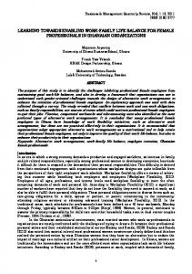
The RUL is defined as the “length from the current life to the end of the useful life”. The keyword is ‘useful’. A better way to understand the RUL is to define the exact time between the present time and a point when the system is useless and actions must be taken to make it useful again. Usually defining that time precisely is impossible; therefore, all good RUL estimations should include three output values: time to failure, deviation of the estimation and the state, when it is not possible to predict the RUL. Defining the RUL is tricky and requires many steps. Figure 16 shows the process from acquisition to maintenance decision-making. Note that the RUL is always based on risk assessment; without considering the risk, the RUL calculation can be meaningless, as no-one wants to run the machine to failure. As illustrated in Figure 2, there are two ways to prolong the life of the machine. If faults are seen early, it is possible to take counter measures to correct abnormal behaviour and prolong the RUL, sometimes even dramatically. Counter measures can be as simple as adding more lubrication to the bearing or correcting misalignment of two shafts connected by a coupling. These types of defects should be detected early in order to fix the problem before any sec- ondary failures occur, or it will progress from defect to failure. In the future, it might be possible to do this automatically by making actuators act according to the output of diagnostic tools. This type of self-maintenance or engineering immune systems can be the missing element linking maintenance and production (Hines & Usynin, 2008; Lee et al., 2014).
Figure 2: Degradation level of the machine Most machines are not detached from the production line immediately after failure and usually it is not even wise to repair them as soon as possible. Standard procedure is to prolong the life by temporary repair or a “quick fix”With 6
accurate estimation of the RUL, it might be possible to prolong the life of the machine by online maintenance or by relieving the operational stress, as illustrated in Figure 3. If this is successful, the maintenance task could be scheduled for a more appropriate moment in the future, thus supporting and optimising production.
��� ����� ���
������
����� ������� ��� �
�� �������� ������
� �� �� �������
������� �� ��� ���
�� �
���
Figure 3: Using operational data to determinate RUL. Usually prognostics comes after diagnostics, but Figure 2 illustrates this is not always the case. Machines can degrade without any particular fault (cracked tooth in gear or dent on a bearing). Faults like a bearing spalling or worn teeth in a gear can start degradation; it can progress a long time before any faults can be seen with diagnostic tools. In these cases, the machine might degrade to a point where it suddenly fails. (Gebraeel et al., 2005) investigated bearings residuallife distributions by running bearings to failure (accelerated test). They used a Bayesian approach to combine reliability characteristics of a devices population and real-time sensor information (Gebraeel et al., 2005)This is one example of performing prognostics without diagnostics. However, after a certain period, degradation will usually cause a failure that can be diagnosed to a particular component or a location. At this point, prognostic tools might be able to predict the RUL more accurately.
7
Figure 4: Which one is RUL?
8
2
Physics-based approach
Today, the model-based approach can be used for maintenance purposes, especially condition monitoring. The main advantage of this approaches to CBM over a data-driven approach is the ability to incorporate a physical understanding of the monitored system (Luo et al., 2003). Data-driven models miss the link between data and the physical world, thus questioning the reliability of the algorithm, but physical models make the prediction of results intuitive because of their use of cause-effect relationships. Their main drawback is the effort required to develop them. Moreover, they require assumptions of complete knowledge of the physical processes; parameter tuning may require expert knowledge or learning from field data. Finally, such high fidelity models may be computationally expensive to run. On the one hand, these models are very useful for describing the behaviour of time-varying systems, taking into account different operating modes, transients, and variability of environmental conditions. On the other hand, the greater the complexity of the model, the greater the effort required to develop and validate it (Galar et al., 2013). This calls for more computational resources. Thus, a limit in the complexity of the physical model should be defined. This section is organised as follows: first, it presents some methodologies for physics models; then, it discusses top layer prediction models; finally,it suggests applications of the models for diagnosis and prognosis.
2.1
Physics based methodologies
The main methodologies are physical modelling, which covers the formulation of a system with equations and damage modelling, and degradation modelling, which consists of modelling the evolution of damage over time. 2.1.1
Physical modelling
Physics-based models typically involve building technically comprehensive theoretical models to describe the physics of the system and failure modes, such as crack propagation, wear corrosion and spall growth, among others. These models attempt to combine system-specific mechanistic knowledge, defect growth formulas and condition monitoring data to provide “‘knowledge-rich” outputs. The physics-based methodologies depend on a fundamental understanding of the physics-of-failure of the system. The objective of such models is to represent the behaviour of engineered systems. The parameters of the models can be related to the system parameters so that the model is a good representation of reality . This feature makes physical models able to predict the future state of the system by means of simulations. The models are determined from the physics of the system and expressed by means of either ordinary or partial differential equations (Isermann & M¨ unchhof, 2011). These equations can be classified as the following: • Balanced equations (i.e. chemical reactions) 9
• Physical or chemical equations of state (i.e. equations relating state variables) • Phenomenological equations (e.g. Fourier’s law of heat conduction) • Interconnected equations (e.g. Kirchner current law) Once a set of equations is obtained, the theoretical model is defined. Complex equations are simplified by means of linearisations, approximations with lumped parameters, and order reductions, amongst others (Isermann & M¨ unchhof, 2011), making mathematical treatment feasible. Then, the final equations are solved using different numerical methods. If necessary, the outputs of the simulation can be used as inputs of the model for further calculations (Bagul et al., 2008). For each engineered system, an entirely new model and algorithm needs to be created to estimate the RUL. It is often difficult to accurately build a theoretical model for a physical system with prior principles in real world applications. (Engel et al., 2000) discuss some practical issues of accuracy, precision, and confidence of RUL estimates. Because of these difficulties, the uses of physical model-based methodologies are limited. (Isermann, 2006) proposes a scheme for fault detection following a modelbased approach, which in Figure 5. Both input U and output Y signals from a system are analysed and relations between them are represented by a mathematical model. Then, features such as state variables x, parameters θ or residuals r are compared with those corresponding to the nominal or healthy conditions of the system with the objective of obtaining the symptoms s that give information about the defective state of the system.
Figure 5: Scheme of model-based fault detection (Isermann, 2006)
10
An appropriate understanding of the faults that occur in the studied system as well as their effect is needed to develop the physical model correctly. Various techniques such as the inspection of the real system, the understanding of the physics and a fault-tree analysis, among others, can be used. The following different reasons for the appearance of a fault should be considered (Isermann, 2006): • Inappropriate design of the system • Incorrect assembly • Inappropriate operating conditions • Lack of maintenance • Ageing • Corrosion and wear during normal operation Not just the kind of fault, but also its evolution should be taken into account in diagnosis. Fault evolution can be divided into three types: abrupt faults, incipient faults and intermittent faults, as shown in Figure 6.
Figure 6: Time evolution of a fault (Isermann, 2006) (Isermann, 2006) indentifies three model-based fault detection methods: parity equations, state estimation and parameter estimation. Table 1 shows the properties of each group. In contrast, (Sikorska et al., 2011) say model-based approaches are focused on the applications and failure modes; therefore, methods cannot be classified.
11
Observation of state is a common technique in physical modelling. The formulation of a state-space model is given by the following expressions for a linear time-invariant process: criteria
assumptions model structure model parameters disturbance models for unknown inputs noise stability of detection scheme excitation by the input detectable fault abrupt drift incipient single faults multiple faults
parity equations
state estimation static output observer observer
parameter estimation
exactly known known, constant
exactly known known, constant
exactly known
exactly known
known unknown, time-varying exactly known
small no problem
small depends on no problem design additive faults: no, multiplicative faults: yes
additive faults: no, multiplicative faults: yes
medium no problem additive faults: no, multiplicative faults: yes
yes yes yes yes SISO: no, MIMO: yes
fault isolation
yes yes yes yes SISO: no MIMO: yes MIMO: yes
additive multiplicative
yes no
yes no
yes yes yes yes SISO: yes MIMO: yes SISO: yes MIMO: yes yes yes
problematic
problematic
unproblematic
many classes possible yes small / medium
limited no medium
many classes possible straightforward medium / larger
yes
yes
general robustness parameter changes nonlinear processes static processes computational effort closed loop
MIMO: yes
yes, external excitation
Table 1: Comparison of model-based methods (Isermann, 2006) State observers are one of the most used techniques in physical modelling. The formulation of a state-space model is given by the following expressions for a linear time-invariant process: x˙ (t) = A x (t) + B u (t)
(1)
y (t) = C x (t)
(2)
12
where x (t) is the state vector, u (t) the input vector, y (t) the output vector, A the state matrix, B the input matrix and C the output matrix. Assuming the structure and the parameters of the model are known, a state observer can be used to estimate the state variable by means of the input and output vectors as shown in: ˆ˙ = A x ˆ (t) + B u (t) + H e (t) x (3) ˆ (t) e (t) = y (t) − C x
(4)
where e (t) is the error vector and H is the observer matrix. A scheme of this state-space formulation appears in Figure 7.
Figure 7: Process and state observer (Isermann, 2006) The presence of faults in the system modifies the above formulation. The state-space equations considering both additive faults and disturbances are the following: (5) x˙ = A x (t) + B u (t) + V v (t) + L fl (t) y (t) = C x (t) + N n (t) + M fm (t)
(6)
where L and M are the faulty entry matrices, fl (t) and fm (t) are the additive faults, v (t) and v (t) are the disturbance vectors, and N and N are the disturbance matrices. A similar formulation for other kind of faults, such as multiplicative faults, appears in (Isermann, 2006). Equations 1 to 6 are formulated for linear systems. Many systems cannot be solved using a linear sum of independent components, a nonlinear relation between the states of the systems is required. The general state-space formulation for a nonlinear system is given by x˙ = f (x, u, t) 13
(7)
y = h (x, u, t)
(8)
where f and h are nonlinear functions that relate the state vector, the input vector and time with the state derivative vector and the output vector. Another commonly used technique is Finite Element Analysis based on the Finite Element Method (FEM), a numerical technique for the resolution of differential equations. This method uses the division of domains into small subdomains, known as finite elements and has the following advantages (Reddy, 2005) • Accurate representation of complex geometry; • Inclusion of dissimilar material properties; • Easy representation of the total solution; • Capture of local effects. This subdivision process is carried out using normalised elements such as cubic elements, tetrahedrons, prisms, etc. In the field of mechanics, this numerical resolution technique is used for the analysis of stress, deformations, fatigue calculations etc. 2.1.2
Degradation modelling
Failure evolution and the way some failure modes initiate or aggravate others should be defined to predict the future response of a system and determine its RUL. Models for failure degradation can be classified as deterministic or stochastic. 2.1.2.1 Deterministic models Crack propagation failure modes are the most commonly developed behavioural models for prognostics (Sikorska et al., 2011). Crack propagation follows a three-stage process, as shown in Figure 8. The first stage represents crack initiation and is the phase in which short or small cracks appear. In the second stage, known as the propagation phase, the size of the crack grows progressively; final failure occurs in the third and last stage, called fast crack propagation (Pugno et al., 2006). This section presents some methods used to represent crack growth due to repeated loads. It also introduces several models related to temperature-related failure, such as the Coffin-Manson model, the Arrhenius equation and the Eyring equation. 2.1.2.1.1 Paris-Erdogan law The most common method to define the evolution of the growth of a subcritical crack under a fatigue stress regime is the Paris-Erdogan law, expressed as: da m = C · (ΔK) (9) dN 14
Figure 8: Fatigue crack growth (Pugno et al., 2006) where a is the crack length, N is the number of load cycles, n is the current iteration, ΔK is the range of the stress intensity factor, and C and m are the socalled Paris’ constants. This law represents the crack growth in the second stage, so it is valid for those values of ΔK that fulfil the condition ΔKth < ΔK < Klc , where ΔKth is the fatigue threshold and Klc the fracture toughness of the material assuming the ratio of the minimum and maximum stress in a cycle R is equal to 0. Paris’ law loses its accuracy in the deviations of stage 3, where a high dependence on the value of R is observed. Many variations have been to adapt this law to other conditions; these include the Foreman equation, the Walker equation and the McEvily equation. 2.1.2.1.2 Foreman equation A common equation used for stress effects in both stages 2 and 3 is the Foreman equation; it take R is expressed as m
B · (ΔK) da = dN (1 − R) · (Klc − ΔK) where B is a parameter.
15
(10)
2.1.2.1.3 Walker equation A method for determining the crack growth with values of R ≥ 0 is the Walker relationship, given by m
A · (ΔK) da = m·(1−λ) dN (1 − R)
(11)
where A and m are the coefficients used in Paris’ law for R = 0, and λ is a material constant. 2.1.2.1.4 McEvily equation To model the rate of fatigue crack growth for short cracks, (McEvily et al., 1991) propose the following: da 2 = D · (ΔKef f − ΔKth ) (12) dN where D is a material constant, ΔKef f = Kmax − Ko , Kmax is the maximum load, and Ko is the crack-tip opening load. The authors modify this expression to capture the evolution of cracks from short to long sizes, introducing a term to reduce the effective stress intensity factor as the crack develops. The final expression is the following: � � �2 � da = D · Kmax − 1 − e−k·l · Kopmax − ΔKth (13) dN where k is a parameter, l is the length of the crack and Kopmax is the crack opening level for a long crack,a function of the ratio of the minimum and maximum stress in a cycle, R. 2.1.2.1.5 Coffin-Manson model The Coffin-Manson model is used to determine the crack growth due to repeated temperature cycling and is expressed as (Cui, 2005): � � EA 1 −a −b N = A · f · ΔT · exp · (14) k Tmax where N is the number of cycles to fail, A is a coefficient, f is the cycling frequency, a is the cycling frequency component, ΔT is the temperature range in the cycling process, b is the temperature range component, EA is the activation energy, k is the Boltzman’s constant and Tm ax is the maximum temperature reached in each cycle. 2.1.2.1.6 Arrhenius equation The Arrhenius equation is a empirical model that relates the temperature with time to failure. This equation is given by � � EA tf = F · exp − (15) k·T where tf is the time to failure if the process is being carried out at the temperature T , and F is a coefficient. 16
2.1.2.1.7 Eyring equation The Eyring equation not only takes temperature into account but also considers stress, using variables such as voltage or current, among others. The equation is expressed as � � � ΔH C α (16) + B+ · S1 tf = A · T · exp k·T T where S1 is the stress variable, and A, α, B and C are parameters. The Eyring equation � has an advantage in many stresses can be included by adding the term � D+ E T · Sn to the exponential for each stress Sn . 2.1.2.2 Stochastic models Stochastic models include Markov chains, hidden- Markov models and semiMarkov processes. 2.1.2.2.1 Markov chain A Markov model is a stochastic model based on the Markov property and is used when the state of a system is fully observable. It assumes the probability distribution of a state depends only on the distribution of the previous state. This assumption can be formulated as P (wn | wn−1 , wn−2 , . . . , w1 ) ≈ P (wn | wn−1 )
(17)
where {w1 , w2 , . . . , wn } is the sequence of states. Thus, the joint probability can be calculated by this theory as P (w1 , . . . , wn ) =
n
p (wi | wi−1 )
(18)
i−1
2.1.2.2.2 Hidden-Markov model A hidden Markov model (HMM) is a kind of Bayesian network based on a finite number of states linked by Markov chains with a set of transition probabilities, as seen in Figure 9. It is used when the states are partially observable. An HMM is denoted by λ (A, B, π) and defined by these parameters (Ocak & Loparo, 2004): • N : number of states • A = [aij ]: transition probability distribution, where aij = p{qt+1 = j|qt = i},
1 ≤ i, j ≤ N
(19)
where qt is the current state. • B = [bj (k)]: observation probability distribution of each state, defined as bj (k) = p{ok |qt = j},
1 ≤ j ≤ N,
1≤k≤M
(20)
where ok is the kth observation and M is the number of observations. 17
• π = [πi ]: initial state distribution, defined as πi = p{q1 = i},
i≤i≤N
(21)
Figure 9: Example of HMM with four states (Ocak & Loparo, 2004) HMMs are useful to define more than one stage of degradation. Knowledge of the failure itself is not required but it does not deal with previously unanticipated faults. It should be noted that HMMs need a large number of data for training, making this a computationally expensive technique. 2.1.2.2.3 Semi-Markov process Let Z = (Zn )n∈N be a stochastic process, S = (Sn )n∈N the successive time points when the state changes occur in the stochastic process and J = (Jn )n∈N the chain with the records of the visited states at these time points. If the following equation is verified P (Jn+1 = j, Sn+1 − Sn = k | J0 , . . . , Jn ; S0 , . . . , Sn ) = = P (Jn+1 = j, Sn+1 − Sn = k | Jn )
(22)
the stochastic process Z is a semi-Markov process (Limnios & Barbu, 2008).
2.2
Methods for top layer prediction
This approach uses a top layer prediction algorithm based on the models describing the nominal operating mode of a system and modelling the degradation phase. This top layer involves one or more of the following: adaptive filters, parameter estimation and artificial data point insertion. 2.2.1
Adaptive filters
There are many kind of adaptive filters, being the most frequently used ones being Kalman and particle filters.
18
2.2.1.1 Kalman filter Kalman filters are predictor-corrector techniques that use a model of a system and measurements from the real system for the estimation of unmeasured states of a process. They are classified as recursive Bayesian estimators. The main kinds of Kalman filters are the following: • Kalman filter (KF) • Extended Kalman filter (EKF) • Unscented Kalman filter (UKF) The difference between KF and EKF is that the former is used for linear time-discrete processes whereas the latter is applied to nonlinear time- discrete processes that can be linearised. UKF is used in highly nonlinear models where EKF performs poorly. Both KF and EKF use the algebraic Ricatti equation to find the solution instead of the Bayes theory used in UKF. This distinction creates a need to initialise the covariate matrices, a limitation of these methods. For applying KF a linear time-discrete process is necessary: xk = Ak xk−1 + Bk uk + wk−1
(23)
y k = Ck x k
(24)
˜ k = yk + vk y
(25)
where k is the actual point in time and k − 1 is the immediate past time point, xk is the vector of actual states, uk is the vector of inputs, yk is the vector of ˜ k is the vector of measured outputs, wk is the process actual process outputs, y noise vector and vk is the output noise vector. These last two noise vectors are assumed to be zero mean Gaussian with covariance Qk and Rk , respectively. KF, as well as the other kinds of Kalman filters, consists of two steps: predictor and corrector. The predictor step computes an a-priori estimate of the ˆ− states at the current time x k using the last state estimate and an estimate of the error covariance: ˆ− ˆ k−1 + Bk uk (26) x k = Ak x T P− k = Ak Pk−1 Ak + Qk
(27)
ˆ− x k
where is the a-priori estimate vector of the states and Pk is the estimation of the covariance of the measurement error. The second step corrects this estimation by incorporating the most recent ˆ k is given by: measurement. The updated state estimate vector x � �−1 − T T K k = P− k C k C k Pk C k + R k
(28)
� � ˆ− ˆ− ˆk = x ˜ k − Ck x x k + Kk y k
(29)
Pk = (I −
K k C k ) P− k
19
(30)
ˆ k is obtained, y ˆ k can be calculated directly. where Kk is the Kalman gain. Once x ˆ k and Pk are stored for the prediction of the next time period. Both x EKF uses the same prediction-correction steps to make estimations for a nonlinear system that can be linearised using Jacobians. Let a nonlinear system be defined as: (31) xk = f (xk−1 , uk , k) + wk−1 yk = h (xk , uk , k)
(32)
˜ k = yk + vk y
(33)
where f and h are generic nonlinear functions that relate the past state, current input vector and current time with the current state and the current output. In this case, the Jacobian matrices Fk and Hk of functions f and h are needed to carry out the prediction and correction steps: � ∂f �� (34) Fk = ∂x �(ˆxk ,uk ,k) � ∂h �� Hk = ∂x �(ˆxk ,uk ,k)
(35)
Thus, the prediction step is carried out as ˆ− xk−1 , uk , k) x k = f (ˆ
(36)
T P− k = Fk−1 Pk−1 Fk−1 + Qk
(37)
and the correction step is carried out as � �−1 − T T K k = P− k Hk Hk Pk Hk + Rk �
�
ˆ− ˆk = x ˜k − h x ˆ− x k + Kk y k , uk , k Pk = (I −
Kh Hk ) P− k
��
(38) (39) (40)
In addition to state estimation, EKF is also used for parameter estimation by running two EKFs simultaneously, in a process called joint or dual estimation (Ji & Brown, 2009). In the EKF, the nonlinear process is linearised to obtain the approximate solution using a Taylor approach and the Jacobians of the nonlinear functions. In contrast, UKF eliminates some of the deficiencies of this kind of linearisation when solving the state estimation problem (Candy, 2009). UKF uses a statistical linearisation approach with the original nonlinear model. A set of -points is used to specify the state. These points take the mean and covariance of the prior Gaussian distribution of the states. In the propagation of these -points, the posterior mean and covariance are captured accurately with errors only in the third and higher order moments. The UKF process is shown in Figure 10.
20
Figure 10: UKF process scheme (Candy, 2009)
21
2.2.1.2 Particle filters Particle filtering implements Bayesian estimators by means of Monte Carlo simulation. The technique uses a number of hypothesised states of the studied system, known as particles, which are samples of the unknown states of the system and have weights attached to them. These weights can be considered as the probability masses estimated using Bayesian recursions (Candy, 2009). Like Kalman filters, particle filters use a two step procedure; a schematic comparison is shown in Figure 11. First, particles are generated following a Monte Carlo approach, taking into account a predefined probability distribution. Next, weights are normalised. Then, only particles with high values of weight are considered, and the others are neglected. Consequently, weights have a great importance since they contain probabilistic information about each particle. This process is called resampling and its main objective is avoiding the situation in which all weights but one are close to zero (Arulampalam et al., 2002). Once resampling is completed, the states are estimated using the new samples. At this point, the whole process is iteratively repeated, using the probability distribution determined by the resampled particles after one iteration to generate new particles in the next iteration. The advantage of particle filters over Kalman filters is that sufficient samples yield an optimal estimate (Khodadadi et al., 2010).
Figure 11: Comparison between particle filter and Kalman filter algorithms (Khodadadi et al., 2010)
22
2.2.2
Parameter estimation and system identification
At times, the process model of a system describing the relationship between inputs and outputs is not known at all, or some parameters are unknown. In these systems, identification methods are used to adjust the parameters of a predefined model. The system identification process has the following steps (See Figure 12). 1. The data framework is defined: first, the conditions of data acquisition are determined in an experimental design; next, experimental data in those conditions are captured from the real system using sensors. 2. The model to be used for system identification must be defined as well. As mentioned, linear or nonlinear models can be used, depending on the complexity of the system being modelled. 3. A criterion function for the parameter estimation is defined to reflect how well the model fits the experimental data. Criterion functions are usually related to error measures. (Chen et al., 2013) present some examples of these functions, such as the mean square error, mean absolute deviation and mean power error, among others. 4. The parameters are computed using data from the system, and the predefined formulation of the model and criterion function. 5. Once the parameters are estimated, the model is validated. If the parameter estimation proves correct, the next step is system identification. If it is not correct, some or all previous steps must be carried out again and modified to improve the parameter estimation. System models can take linear or nonlinear approaches. There are many techniques of parameter estimation (Nelles, 2001); the least squares method is arguably the best known. The method obtains the minimum value of the sum of the squared residuals, where the residuals are the difference between the measurements and the value provided by the model. The least square method can be used to fit data to a simple linear regression or a multivariate linear regression; it can also fit data to some nonlin- ear regressions, such as polynomial or exponential regression. Other techniques should be used for other nonlinear regression kinds, including logarithmic regression or trigonometric regression. Figure 13 is a schematic representation of some of these methods. 2.2.2.1 Proportional hazard model The proportional hazards model (Bagul et al., 2008) is frequently used for condition monitoring. It consists of a function formed by the product of a baseline hazard rate and a positive function described by covariates (functions of time that can be any condition variables) and regression parameters, with the positive function an exponential. Thus, it is expressed as: h (t) = h0 · (t) eγ1 ·x1 (t)+···+γp ·xp (t) 23
(41)
Figure 12: Scheme of the identification process
24
Figure 13: Identification methods (Isermann, 2006) where x1 (t) , . . . , xp (t) are the covariates, γ1 , . . . , γp are the model parameters that must be estimated, and h0 (t) is the baseline hazard rate, with represents the change in the risk during time as a baseline for every covariate. However, the use of the this technique is subjected to the fulfilment of a series of conditions. The following assumptions are made: • Times to failure are independent and identically distributed; • Covariates have a multiplicative effect on the baseline hazard rate; • Individual covariates are independent; • The effect of the covariates is assumed to be time independent; • All influential covariates are included in the model; • The ratio of any two hazard rates is constant with respect to time. 2.2.3
Artificial data point insertion
It may not be possible to get data for some (or all) faulty conditions from a real system for the following reasons: • Security: some faults put both the asset and the people using it at risk. • Cost: the development of a fault in a component in some equipment, for example, an aircraft, can be very expensive.
25
Figure 14: Model-based FDI • Environmental issues: the effect of a fault can be detrimental for the environment. The response of the system in these conditions is unknown, but the use of a physical model allows us to estimate. A complete data set that covers the response of the system in both nominal and faulty conditions can be obtained by using both healthy data from the real system and artificial data created by a physical model.
2.3
Model-based diagnosis
Model-based diagnosis can be carried out using state observers or parameter estimation; it can also be done using parity equations and residuals. A scheme for model-based fault detection and identification using this last technique is shown in Figure 14. The residuals are the difference between the acquired signals from the system and the signals obtained by the physical models. This difference gives information about the current status of a system, taking as a basis the nominal operation conditions introduced in the physical model. Several researchers have investigated model-based diagnosis. (Kiral & Karag¨ ulle, 2003) propose a finite element model with localised defects for the diagnosis of rolling element bearings. They amplify the contact forces using a predefined constant when the bearing contact is produced in a damaged area. (Immovilli et al., 2012) present an analytical model for a bearing to simulate its response when external harmonic excitation is applied. They use an airgap variation model to study the relationship between current and vibration in the induction machines where the bearings are located. (Bourbatache et al., 2013) use a discrete element model to characterise the electromechanical behaviour of a ball bearing in both healthy and faulty conditions. In this work, the electrical response is shown to be very useful for geometric defect detection. Using a 2 DOF model, (Rafsanjani et al., 2009)reproduce the transient force that occurs when a rolling element bearing comes into contact with a defective 26
surface creating a series of impulses that repeat the characteristic frequencies of the elements of the bearing. (Tadina & Bolteˇzar, 2011)develop a 2D model of a bearing in which defects are modelled as geometric changes. In this case, a fault in a race is modelled as an ellipsoidal depression whereas a fault in a ball is modelled as a flattened sphere. (Patil et al., 2010)use the same 2 DOF approach and model defects in races as half sinusoidal. Vibration response is used in order to detect those defects as well as determine the effect of the position and the size of the defect. (Cong et al., 2013)propose a mathematical model for the dynamic load analysis of a rotor-bearing system, taking into account geometrical faults in both inner and outer rings. They conclude that envelope spectrum expressions caused by different amplitudes of alternate and determinate loads can increase the difficulty of the fault detection process. (Sawalhi & Randall, 2008)present a 5 DOF model for a rolling element bearing in which they consider the rolling elements as angularly equidistant; they also propose a 6 DOF model for a gear, and use the model to obtain the response of a gearbox test rig. (Li et al., 2013) present two analytical models for a rolling element bearing, one with 2 DOF and another one with 6 DOF. They conclude the more complex model reaches a better diagnosis because it is able to detect faults earlier. They also take advantage of the frequency spectrum of the bearing vibration to determine the position of the fault. (Cao & Xiao, 2008) develop a model for spherical roller bearings considering two defect kinds: waviness in all the modelled elements of a bearing and point defects. This last kind of damage is limited to moderate to large sizes because of the formulation employed for the contact modelling. (Shao et al., 2014) propose a new kind of localised surface defect modelling for cylindrical roller bearings. They consider different contact conditions between the rollers and the defect in the race and study their effect using a 2DOF model. (Isermann, 2011)presents fault diagnosis processes for electrical drives and actuators, fluidic actuators, pumps, pipelines, robots, machine tools and heat exchangers, giving examples of system modelling, parameter estimation and fault detection. (Khanam et al., 2014) identify faults in rolling element bearings by applying a Kalman filter to a 2 DOF model. They use spectrum analysis for fault diagnosis, taking advantage of the denoising carried out by the Kalman filter.
2.4
Model-based prognosis
Model-based prognosis is usually carried out after diagnosis, when faults have been detected, isolated and identified. The damage state of a system is estimated and its future degradation is predicted to determine the remaining useful life of the system. Following this approach, (Daigle & Goebel, 2011) define a scheme of model-based prognosis for the estimation of end of life (EOL), as shown in Figure 15. Note: there are two ways of estimating the RUL of a system. The one shown in Figure 15calculates the EOL as a probability distribution at a given predic27
Figure 15: Model-based prognosis (Daigle & Goebel, 2011) tion time. The other obtains a deterministic RUL, a unique value of time when the system crosses a predefined threshold. (Saha et al., 2009a) emphasise the need to use a probabil- ity density function to determine the RUL instead of just a obtaining a mean time-to-failure value. In their work, they analyse the degradation of isolated gate bipolar transistors taking advantage of particle filters for the prognosis of these elements. There are many references in the literature to the methods presented in 2.1and 2.2. (Kacprzynski et al., 2004)study the propagation of a single fatigue crack in a helicopter gear, using a finite element model and Paris law. They use vibration features with the aim of reducing the uncertainty levels due to loading, material properties and modelling, thus improving the models prediction (Li et al., 1999)use a deterministic propagation model as a variation of the Paris formula, establishing the defect severity of a bearing by means of the surface area instead of the defect length. They set the parameters of the damage model using a recursive least square error method. (Li et al., 2000) introduce a lognormal random variable to the aforementioned deterministic propagation model, in such a way that a stochastic defect propagation is considered. Hence, both the mean and the variance of the defect propagation are estimated. A similar stochastic approach for the estimation of the defect propagation is considered by (Ray & Tangirala, 1996).The authors use the extended Kalman filtering to compute the stochastic damage state; they predict the remaining useful life of the studied system in a way that is valuable for maintenance decision making. (Oppenheimer & Loparo, 2002) combine a physical model based on observers with a life model to determine the remaining life of a system. They also use a material crack growth law, in this case, the Forman law, to estimate the time needed for a crack to grow from its current size determined by the observer to a predefined critical crack size (Qiu et al., 2002) study the prognostics of a bearing considering the machine element as a 1 degree-of-freedom system and using three different damage modes: linear damage mode, damage curve approach and double linear damage rule. The authors conclude that the last two methods predict accurately the remaining life of the system but the former does not give good predictions. ((Cempel, 1987) apply a physical model with four different degradation trends to the forecasting of the behaviour of a high power fan and a railroad diesel engine.
28
(Chelidze & Cusumano, 2004) suggest a procedure for the study of the evolution of a hidden damage in a system, assuming that the damage process occurs much slower than the observable dynamics of the system. They apply this procedure to predict the battery discharge of an electromechanical system. (Luo et al., 2003) divide the model of a system into some variables related to the fast behaviour of the system and other variables related to the slow damage degradation. After creating the model and carrying out simulations under random loads, they construct prognostic models for different operating loads and use an interacting multiple model estimator to estimate the damage variable. The authors apply this theory to an automotive suspension system. (Adams, 2002) introduce first order nonlinear differential equations in a mathematical model representing the dynamics of a system with the objective of defining the damage accumulation. The authors assume the damage state equations are functions only of the damage variables, neglecting the effect of the state vector in the damage evolution. ((Lesieutre et al., 1997) state that a mechanical system is formed by a hierarchical collection of interacting parts, from material and component levels to the system level. They consider the damage state at every level of the hierarchy. (Medjaher & Zerhouni, 2009) propose the use of residuals for failure prognostics. They apply this approach to the estimation of the RUL in a hydraulic system in which a physical degradation equation is given to determine the only fault condition considered, namely, the increase of the resistance of a valve. The authors project the values of the residuals related to flow conservation and pressure conservation to determine the RUL. (Swanson et al., 2000) use a Kalman filter to track the modal frequencies of a steel band, which has a notch where a crack is propagated because of the applied vibration excitation. They use these modal frequencies to determine indicative failure. Next, they examine the evolution of these frequencies to see if they are maintained in a stable state (healthy case) or if they diverge from the stable state (faulty case); finally, they perform prognosis. (Bartram & Mahadevan, 2013) present a diagnosis and prognosis analysis for a hydraulic actuator system. They consider the seal in the actuator to be the component that develops degradation because of wear. The volume of removed material is modelled as a function of the frictional forces on the seal, the sliding distance and the wear rate. The particle filter method is applied to the model of the system to get information for both diagnosis and prognosis. (Khan et al., 2011) use particle filters to estimate the RUL of steam generators in nuclear reactors. For that purpose, they use measures of the eddy currents on the generators. Predictions for flaw growth have an increasing uncertainty at future times, so this is corrected by means of an auto-regressive model. (Orchard & Vachtsevanos, 2009) apply particle filters to the diagnosis and prognosis analyses of the plate of a planetary gearbox, taking the evolution of an axial crack as the fault degradation. The authors state that deterministic models for damage evolution give good long-term predictions but are insufficient for the on-line determination of confidence intervals. The use of measured data is crucial to remedy this lack. (Cadini et al., 2009) show the ability of particle filters to be used for the estimation of the states of a nonlinear system. The authors apply this theory to the problem of crack propagation 29
taking as a basis Paris law. They modify the particle filter algorithm with the aim of obtaining an appropriate RUL estimation. (Saha et al., 2009b) compare different methods to estimate RUL. They emphasise the advantages of combining relevance vector machines and particle filters over other techniques such as ARMA and EKF. (Lorton et al., 2013) use a Markovian approach to approximate the RUL of both a shock-absorber system and a pneumatic valve for aeronautics. They present a two-step procedure, in which a conditional distribution of the system is calculated at prognosis time and the reliability is subsequently computed. (Gaˇsperin et al., 2011) calculate the time when a gear reaches a critical stage. As they consider the dynamics of the element to be stochastic, they estimate the RUL of the gear propagating the distribution of the current system state by means of a degradation model. The Expectation-Maximitation (EM) algorithm, which is used for the estimations, employs a Kalman filter.
30
3
Data Driven Approach
Some reviews look at all the various techniques used for condition monitoring, notably basic signal processing techniques and data-driven techniques. One review, by Jardine et al. (Jardine et al., 2006), focuses on traditional statistical condition monitoring methods (e.g. Waveform data analysis), all of which can be considered data-driven models. He explains in detail all aspects of condition based maintenance from data acquisition to maintenance decision-making. However, the review appeared in 2006 and there have been many developments in AI since then. In addition the review deals with methods at a machine level; it does not look at components or precise methods developed for them. A more recent review by Lee et al. (Lee et al., 2014)focuses on rotating machines and classifies different methods that are appropriate for a certain component (e.g. bearings). It also covers more AI approaches than Jardine et al. Li et al. (Si et al., 2011) review pure statistical data driven approaches. This review is discussed in Chapter 19. Figure 16 illustrates the flow of condition based maintenance, with all three approaches seen (also Physics-Based Models) in the flow. Roughly speaking, data driven machines use either statistical techniques or AI techniques. The former include reliability models and techniques to handle vibration signals. Since basic signal processing methods are described in almost every handbook of condition monitoring, we will only mention them briefly. Although these methods are still in use and very effective in most applications, we are addressing techniques that might be mainstream methods in the future. Data driven techniques are moving towards machine learning and data mining techniques. Anomaly detection techniques are especially interesting since they require little human interaction in data analysis. That said, the basic protocol, from data acquisition to maintenance decision making, is not likely going to change, making it good to understand the steps in Figure 16.
3.1
Preprosessing The Data
preprocess is a process where inputs of a data is altered to to produce output that is used as input to another program or algorithm. 3.1.1
Data Available
Data can be divided into two groups: event data and condition monitoring data. Event data consist of events affected by the system or its behaviour, including information on what happened, what the causes were and what was done. Event data can be used to complement the condition monitoring data; they help to clarify when something has changed in the system or in its environment. However, event data are seldom used as a part of a condition monitoring system, mostly because they are usually manually entered into the system and therefore prone to errors (Jardine et al., 2006). Condition monitoring data are case specific, but some common data types can be collected from almost every mechan-
31
Figure 16: Flow of Condition Based Maintenance. ical machine, as nearly every machine needs bearings and lubricants (rotating machines). Figure 16 shows most of the data (event and condition monitoring) available for inputs to the RUL algorithms. The common data types for rotating machines are: • Vibration, • Acoustic emission, • Condition of the lubricant, • Speed, • Temperature and • Load. Note that some of these data types are not unambiguous (e.g. speed and load); this means that further assumptions, limitations or additional sensors are sometimes needed to detect them properly. A good review of different types of sensors, how to choose them, and ways to monitor the condition of the machine appears in Cheng et al (Cheng et al., 2010). Their approach is realistic; they also consider ways to implement the sensors into the machine and estimate the cost.
32
3.1.2
Feature Extraction
The usability of methods for CM is highly dependent on the features used or how the data are pre-processed. For vibration and acoustic emission data, performing pre-processing might be even more important than using the correct analytic technique. Condition monitoring is focusing more on feature selection because more advanced machine learning techniques are becoming available; these can easily handle large datasets and this means more emphasis on what is classified as a feature. A few researchers discuss how to choose features and suggest what type of pre-processing should be performed on the data (Iguyon & Elisseeff, 2003; Verma et al., 2013; Samuel & Pines, 2005). Most consider that features should be independent but comparable among data types. Sometimes features are extracted automatically; some neural networks can automatically create features from the raw data. However, this can be computationally costly; therefore, feature extraction remains an important process in condition based maintenance. For some anomaly detection methods (see chapter 3.3) features should be normally distributed. Therefore, some data manipulation should be used (e.g. distributing the data set logarithmically to make it look like a normal distribution). Features can be manipulated in different manners by combining two features (e.g. crest factor) to come up a new feature for detecting anomalies which the source features could not detect independently. This can be useful in another way: more specifically, these types of multivariate features can be used to test if sensors are broken/malfunctioning by, e.g., combining vibration and temperature features at the same location to come up a new feature that can detect a problem. 3.1.3
Noise Removal And Blind Source Separation
Another interesting way of pre-processing the signal is to separate it into its source signals by using machine learning. This process is commonly known as blind source separation or BSS (Comon & Jutten, 2010; Hyvrinen, 1999). BSS tries to solve the common and irritating CM problem of getting rid of noise from unwanted sources. Common methods for this are using time synchronous averaging (TSA) (Jafarizadeh et al., 2008; McFadden, 1991, 1994; Shin, 2011; Halim et al., 2008), using regular filters, working in a time-frequency domain (Antoni, 2006; Antoni & Randall, 2006; Almeida, 1994), or using adaptive noise filters (Randall & Antoni, 2011; Chaturvedi & Thomas, 1982; Tan, 1987). Some advanced methods to filter the signals have been developed (Qiu et al., 2003). However, in principle, noise in a machine is not usually just noise. It is a signal coming from other components and, therefore, can have usual information on the status or health of the machine. And since BSS is only separating the signals, it seems to be a promising tool to pre-process the data. BSS can reduce noise without any a priori knowledge (i.e., using only assumptions) from the machine itself and even locate signals in some cases, making it possible to know which component is producing the signal. So far no-one has been fully successful, but
33
there is some recent progress in creating better BSS algorithms. If BSS is done successfully it would be extremely beneficial to combine BSS techniques with physics-based prognostics models and target the signal to a specific component or use it to calculate more precise features. BSS techniques are more commonly used for separating audio signals and only some researchers have tried to separate pure vibration signals (Gelle et al., 2000, 2001). Usually vibration signals are more convoluted by nature; i.e. there are delays and echoes (Comon & Jutten, 2010). To overcome this problem, the usual assumption is the mutual statistical independence among the unknown sources, also called the iid assumption. This assumption is fully justified in many problems, but standard ICA (Independent Component Analysis) techniques cannot be applied for vibration sources. Convolutive ICA techniques must be employed instead. Convolutive ICA techniques separate the sources e.g. by convolving the mixture signals with multichannel FIR unmixing filters, often chosen to maximise some contrast function of the resulting source estimates. These filters can be expressed either in the time domain (Comon & Jutten, 2010) or in the frequency domain (Comon & Jutten, 2010; Araki et al., 2003; Makino et al., 2005; Ikeda & Murata, 1999; Sawada et al., 2004). The disadvantage of using frequency domain filters is that a scaling and permutation problem occurs, i.e. wrong order and gain might be seen in the source signals (Araki et al., 2003). Antoni has written about the problems that occur when BSS is applied to vibration signals (Antoni, 2005). 3.1.4
Spectral Kurtosis And Kurtogram
Spectral kurtosis (SK) is a way of determining which frequency bands contain a signal of maximum impulsiveness; it is based on a short time Fourier transform (STFT). Figure 17 shows SK measurements from a gearbox submitted to an accelerated fatigue test that demonstrates the usefulness of SK. For example, it can be used as a tool in BSS. To obtain a maximum value of kurtosis, the window must be shorter than the spacing between the pulses, but longer than the individual pulses. (Randall, 2011) Antoni and Randall propose that SK can also detect the precise point at which frequency bands show the best contrast faults from background noise. SK with multiple window length is called a Kurtogram. It can optimise the correct value of SK and, thus, can be very beneficial for many applications. The Kurtogram can be a helpful tool for solving the problem of choosing the most suitable band for demodulation in an envelope analysis (Randall & Antoni, 2011). Figure 18 shows a Kurtogram where maximum SK is achieved when the frequency is 14,0 kHz and the window length is 44. Despite its effectiveness, computing the full Kurtogram can be very costly (Randall, 2011). SK can be used for feature selection in a frequency domain automatically since most the sensitive bandwith is usually where SK reaches the maximum, as in Figure 17. For bearings, these are usually impact frequencies of inner ring, outer ring and ball which can also be manually calculated, if the rotating speed is known. 34
Figure 17: SK of measurements on a gearbox submitted to an accelerated fatigue test (Antoni, 2006)
Figure 18: Kurtogram of a rolling element bearing signal with an outer race fault (Antoni, 2006)
35
3.1.5
Data Fusion
Data fusion can be categorised into three different subgroups based on the stage when data are merged: • Sensor data fusion, • Data fusion and • Information fusion. As Figure 16 indicates, there are many different types of condition monitoring data that can be collected. In sensor fusion, data are collected from similar types of sensors, for example, data can be collected from three vibration sensors and then merged. This can help to reduce the noise or find signals impossible to detect with just one sensor alone (e.g. slowly rotating large machines). Data fusion is usually done by combining pre-calculated features and pre-processed data. Data fusion combines all the condition monitoring data. collected from different types of sensor (e.g. vibration, temperature etc.). The most neglected type of data fusion is information fusion. This fusion is done in a more symbolic way, with the goal of combining or merging condition monitoring data and event data (e.g see Section 3.2.6). Information fusion (see Figure 16) in CM usually occurs in the heads of maintenance personnel, not in a computer; this is still the backbone of maintenance decision making. The ongoing challenge in building CM models is to include all the steps in data fusion, select the appropriate approach for a particular machine and then estimate the RUL without requiring the human inside the loop.
3.2
Statistical Approaches
Statistical data-driven approaches use only available past observed data and statistical models to estimate RUL. A good review of different types of statistical data-driven approaches is provided by Si et al. (2011). They classify approaches into models that rely directly observe data state information and those that do not, as seen in Figure 19 (Si et al., 2011). They conclude it is desirable to develop an RUL estimation model based on very few or no data, for example, for newly commissioned systems with no observed failure data or no previous CM data. They also suggest physics-based models can create enough data to be used with statistical models. Finally, Si et al. discuss the challenge of modelling external environmental variables such as speed or load (see figure 3). Usually statistical methods provide general overall estimates for the entire population of identical units (fleet) and are not useful for individual operating units (Heng et al., 2009). 3.2.1
Regression-Based Models
A linear regression model is perhaps the simplest model to use for CM trending. Among the possible methods for such models, the most popular is random coefficient regression; it uses the CM data to depict the CM path and infer the lifetime 36
Figure 19: Taxonomy of statistical data driven approaches for the RUL estimation (Si et al., 2011) distribution. Linear regression models are the simplest models to characterise the degradation path. In contrast to statistical learning methods (i.e., Bayesian networks; see Section 3.3.1.9), random coefficient regression models can provide a Probability density function (PDF) of the RUL, but a closed-form of such a PDF is only available in some special cases (Si et al., 2011). 3.2.2
Wiener Processes
Wiener processes (i.e., Brownian motion) for degradation modelling are appropriate when the degradation processes vary bi-directionally over time with Gaussian noise. An advantage of the Wiener process is that the distribution of the first passage time (FPT) can be formulated analytically; this is known as the inverse Gaussian distribution. A major disadvantage of the Wiener process-based models is that they only use information contained in the current degradation data and ignore information from the entire sequence of observations (Si et al., 2011). 3.2.3
Gamma Processes
The degradation process can be monotonic. A Gamma process is a natural model for degradation processes in which the deterioration evolves slowly. These type of processes can be caused by slowly progressing corrosion damage or other ageing failures, which are not that common for rotating machines (Kuniewski et al., 2009). 3.2.4
Markovian-Based Models
The assumption of Markov models is that the future degradation state of the item depends only on the current degradation state and the systems state can be 37
revealed by the observed CM information. Therefore, Markovian-based models have been widely applied to estimate the RUL. On the one hand, a Markov model can be divided into several meaningful states (e.g. healthy, okay, and maintenance required); this is much closer to what is used in real-world industry. On the other hand, its conditionally independent assumption can lead to an approximation that is not true-to-life (Si et al., 2011) 3.2.5
Stochastic Filtering-Based Models
The Kalman filtering approach overcomes the problem of using only the last CM readings, since it uses information on the systems history. However, linear and Gaussian assumptions restrict the application of the Kalman filtering approach (Si et al., 2011). The review by Si et al. cites a number of cases where stochastic filtering-based models have been applied. They all have the same drawback: they all need a threshold limit, which not only takes a long time to set appropriately but also changes with machine modifications. 3.2.6
Covariate Based Hazard Models
In many mechanical components, degradation is caused by multiple factors called covariates (temperature, material properties, running speed etc.). These change stochastically and may influence the lifetime. Thus, all the covariates should be included in lifetime modelling (Si et al., 2011). The proportional hazards model is suitable for analysing event data and condition monitoring data together (Jardine et al., 2006; Si et al., 2011). A 1972 paper by Cox et al. has been highly cited in the statistical sciences (Cox et al., 1972). A good review of these models is provided by Kumar and Klefsj¨ o(Kumar & Klefsj¨o, 1994). 3.2.7
Hidden Markov Models (HMM)
HMMs use a stochastic process in which the subsequent states have no causal connection with previous states. Unfortunately, an HMM cannot relate the defined health-state change point to the actual defect progression, because it is impractical to observe a defect in an operating unit (Heng et al., 2009).
38
3.3
Machine learning and Data Mining
Machine learning is a sub-category of artificial intelligence. Its purpose is to learn from data and make better predictions as the training data increases. Machine learning has been defined as a field of study that gives computers the ability to learn without being explicitly programmed (Arthur Samuel). In data mining, information is extracted from data and transformed into an understandable structure for further use. Data mining and machine learning overlap in many ways and their methods to achieve their goals can be the same. The goals differ, however. Machine learning tries to reproduce known knowledge but data mining tries to discover previously unknown knowledge. Obviously, machine learning and data mining represent a huge topic and it is impossible to cover all possible techniques here. In this technical report, the emphasis is on anomaly detection techniques which can be seen as machine learning techniques or data mining techniques depending on the goal. Usually, AI attempts to get the same results as basic signal processing techniques, see (Allen & Mills, 2004; Jardine et al., 2006) or reliability models without having to spend lot of man-hours to do the analysis of the data. Usually AI approaches are based on machine learning or anomaly detection algorithms, but other techniques are available, such as fuzzy logic, that are not dealt with here. 3.3.1
Anomaly Detection
Anomaly detection tries to identify events which do not conform to an expected pattern in a dataset. They are also sometimes called outliers, novelties, noise, deviations and exceptions. Unsupervised anomaly detection techniques detect anomalies in an unlabeled test data set under the assumption that the instances in the data set are normal by looking for cases that fit least to the rest of the data set. Supervised anomaly detection techniques require a data set with data labelled normal and abnormal. This requires training a classifier; the classifier separates machine learning methods from statistical techniques (see Section 3.2). Semi-supervised anomaly detection techniques construct a model representing only normal behaviour. A common challenge in anomaly detection according to Chandola et al. (2009) is how to define normal behaviour, as it keeps evolving; a current notion of normal behaviour might not be sufficiently representative in the future. In addition, the availability of labelled data for training or validation of models can be a major issue (Chandola et al., 2009). The anomaly detection problem is not easy to solve. When it comes to anomaly detection for CM data, researchers have adopted concepts from diverse disciplines such as statistics (Timusk et al., 2008), machine learning (Timusk et al., 2008), data mining (Knight et al., 2005), information theory (Agogino & Tumer, 2006) and have applied them to specific problem formulations. According to Chandola et al. anomaly detection in sensor networks poses a set of unique challenges. The presence of noise in the data makes anomaly detection more challenging, since it must distinguish between interesting anomalies
39
and unwanted noise or missing values (Chandola et al., 2009). For this reason it is essential to choose good features when monitoring the condition of rotating machines (see Section 3.1). A good survey of anomaly detection techniques is by Chandola et al. (2009) and most of the methods mentioned here are discussed in more detail in their technical report (Chandola et al., 2009). However, our techniques and examples are closer to the real problems in condition monitoring. 3.3.1.1 Anomaly Types A point anomaly is an individual data instance that can be considered as anomalous. This is the simplest type of anomaly and is the focus of the majority of research on anomaly detection. A contextual anomaly or conditional anomaly is a data instance that is anomalous in a specific context, but not otherwise. These instances are defined using the following two sets of attributes (Chandola et al., 2009): • Contextual attributes are used to determine the context(machine operating circumstances) for that instance and • Behavioral attributes define the non-contextual characteristics of an instance (e.g. Load or rotation speed). The anomalous behaviour is determined using the values for the behavioural attributes within a specific context. A data instance might be a contextual anomaly in a given context, but an identical data instance could be considered normal in a different context. This property is key in identifying contextual and behavioural attributes for a contextual anomaly detection technique. For CM, this is important since machines can have multiple phases in their duty cycle. Long et al. investigate spacecraft and their RUL using support vector (see Section 3.3.1.5) machines. To improve the algorithm, they point out the difference between point and contextual anomalies (Long et al., 2011). The choice of a contextual anomaly detection technique is determined by the meaningfulness of the contextual anomalies in the target application domain. Another key factor is the availability of contextual attributes (Chandola et al., 2009). For rotating machines, many contextual attributes should be available as long as data are collected systematically and are valid (e.g. time labels are correct for each data set). A third type of anomaly is the collective anomaly which is a collection of related data instances that are anomalous to the entire data set. Long et al. discuss these collective anomalies (Long et al., 2011). 3.3.1.2 Classification Based Anomaly Detection Techniques Classification is used to learn a model (classifier) from a set of labelled data instances (training) and classify a test instance into one of the classes using the model (testing). Classification based anomaly detection techniques operate in a similar two-phase fashion. The training phase learns a classifier using the available labelled training data. The testing phase classifies a test instance as 40
normal or anomalous using the classifier. Classification based anomaly detection techniques operate under the following general assumption: A classifier that can distinguish between normal and anomalous classes can be learnt in the given feature space In the figure 20 is illustrated two different types of classification methods in principle.
Figure 20: Using classification for anomaly detection (Chandola et al., 2009)
3.3.1.3 Neural Network Approach Neural networks (NN) have been applied to anomaly detection in both multiclass and one-class setting. An NN is a model that simulates the structures and functions of the brains neural network. It can learn by modelling complex relationships between inputs and outputs searching for patterns within the neurons. NN models are highly adaptive and can handle non-linear behaviour or unstable processes. NN is a supervised learning technique. Although the technique was discovered in 1943 (McCulloch & Pitts, 1943), it can be considered a fairly new technique since it has made a comeback in the era of computers. Recent use of backpropagation and deep learning has made it a promising technique to build real self-learning AI (Mohamed et al., 2012; Jack & Nandi, 2002). Deep learning can automatically extract high level invariant discriminative features from the raw data. Deep learning is usually used with supervised backpropagation, but it is an unsupervised learning process (Le et al., 2012). Some work has been done to train NN to predict the RUL (Tian et al., 2010; Samanta et al., 2003; Samanta & Al-Balushi, 2003; Paya et al., 1997). Tian et al. use an ANN model with inputs of CM data and failure history. They discuss the usability of physical models, but say that an authentic way of combining them remains a challenge. The limitation of their model is that failure history is suspended; the target is repaired before it fully reaches the faulty state. This is almost always the case in real life, as everybody wants to repair systems before they reach the
41
end of life. Samanta et al. use time domain features. Paya et al. use NN by first pre-processing data using wavelets. 3.3.1.4 Bayesian Network Approach A Bayesian network is a directed acyclic graph tool (DAG) which can present the structure of conditional interdependency relations and probability distributions between variables in one domain system. It aggregates information from different variables and provides an estimate of the expectancy of belonging to either normal or anomalous classes. A Bayesian network database consists of cases with differing probabilities of occurring. Good introductions to Bayesian networks with references are by Cooper and Herskovits (Cooper & Herskovits, 1992) and Heckerman et al. (Heckerman et al., 1995). Bayesian networks have been used for anomaly detection in the multi-class setting. A basic technique for a univariate categorical data set using a naive Bayesian network estimates the posterior probability of observing a class label in a given test data instance. The class label with largest posterior is chosen as the predicted class for the given test instance. The likelihood of observing the test instance, given a specific class and the class probabilities, is estimated from the training data set. Zero probabilities, especially for the anomaly class, are smoothed using Laplace Smoothing. (Chandola et al., 2009) The basic technique can be generalised to a multivariate categorical data set by aggregating the per-attribute posterior probabilities for each test instance and using the aggregated value to assign a class label to the test instance. Several variants of the basic technique have been proposed: network intrusion detection, video surveillance, text data and disease outbreak detection. However, this has not been applied to rotating machines, at least according to Chandola et. al. (Chandola et al., 2009). 3.3.1.5 Support Vector Machine Approach The Support Vector Machine (SVM) is a supervised learning method used to create a line or hyperplane between two sets of data for classification. SVM tries to orient the boundary such that the distance between the boundary and the nearest data point is maximal (Samanta et al., 2003; Jack & Nandi, 2002). Long et al. use SVM the estimate the RUL of a spacecraft. Their method uses point, contextual and collective anomalies as a sign of abnormal behaviour. They select many different features (mean, variance, RMS kurtosis and etc...) as input to their SVM. They also use a statistical method called principal component analysis (PCA) to transform a multivariate data set into a smaller number of uncorrelated variables called principal components. 3.3.1.6 Rule-Based Approach Rule based anomaly detection techniques learn rules that capture the normal behaviour of a system. A test instance not covered by any such rule is considered an anomaly. Rule based techniques have been applied in both multi-class and one-class settings. The multi-class rule based technique has two steps:
42
1. Learning rules from the training data using a rule learning algorithm (e.g. RIPPER and Decision Trees). Each rule has a confidence value proportional to the ratio between the number of training instances classified correctly and the total number of training instances covered by the rule. 2. Finding the rule that best captures the test instance.
3.3.1.7 Nearest Neighbor-Based Techniques The concept of nearest neighbour analysis has been used in several anomaly detection techniques. Such techniques are based on the following key assumption: Normal data instances occur in dense neighborhoods, while anomalies occur far from their closest neighbors (Chandola et al., 2009). Nearest neighbour based anomaly detection techniques require a distance or similarity measure defined between two data instances. Distance between two data instances can be computed in different ways. For continuous attributes, Euclidean distance is a popular choice but other measures can be used. For categorical attributes, a simple matching coefficient is often used but more complex distance measures are also appropriate. For multivariate data instances, distance is usually computed for each attribute and then combined. Nearest neighbour based anomaly detection techniques can be broadly grouped into two categories (Chandola et al., 2009): 1. Techniques that use the distance of a data instance to its k th nearest neighbor as the anomaly score and 2. Techniques that compute the relative density of each data instance to compute its anomaly score. Table 2 lists some of the advantages and disadvantages of using NearestNeigbor techniques (Chandola et al., 2009).
43
Table 2: Advantages and disadvantages of using Nearest Neighbor-Based Techniques Advantages No assumption on the generative distribution for the data Good for Semi-supervised learning since anomaly will not likely settle to a group of training data Straightforward technique for a different types of data Disadvantages If not enough close neighbors to normal instances may fail to label them correctly Anomalies with enough close neighbours are not seen as anomalies Computing distance for each data point takes a lot of computational power Relies on a distance measure between normal data and outliers which can be challenging for the complex data Not suitable for data that have modes with varying density
44
3.3.1.8 Clustering Based Anomality Detection Techniques Clustering is used to group similar data instances into clusters. Clustering is primarily an unsupervised technique though semi-supervised clustering has also been explored lately. Even though clustering and anomaly detection appear to be fundamentally different, several clustering based anomaly detection techniques have been developed. Clustering based anomaly detection techniques can be grouped into three categories. Assumptions of these three categories appear in Table 3. Table 3: Assumptions of different types of clustering techniques. Assumptions 1. 2. 3.
Normal data instances belong to a cluster in the data, while anomalies either do not belong to any cluster Normal data instances lie close to their closest cluster centroid, while anomalies are far away from their closest centroid Normal data instances belong to large and dense clusters, while anomalies either belong to small or sparse clusters
Techniques based on the second assumption consist of two steps. These are: 1. cluster the data using a clustering algorithm and then 2. calculate the distance of each data instance to its closest cluster centroid. The result of this calculation is usually referred as anomaly score. Techniques based on the second assumption can also operate in a semisupervised way; the training data are clustered and instances belonging to the test data are compared to the clusters to obtain an anomaly score for the test data instance. In several clustering-based techniques, distance is computed between a pair of instances, making them very similar to nearest neighbour based techniques (Chandola et al., 2009). Table 4 shows the advantages and disadvantages of various clustering techniques. 3.3.1.9 Statistical Anomaly Detection Techniques Statistical anomaly detection techniques are based on the following assumption, which is: Normal data instances occur in high probability regions of a stochastic model, while anomalies occur in low probability regions. Statistical techniques (usually for normal behaviour) are applied to the data and a statistical inference test is performed to determine if an unseen instance belongs to this model. Instances with a low probability of being generated from the learnt model, based on the applied test statistic, are declared anomalies. 45
Table 4: Advantages and disadvantages of different types of clustering techniques. Advantages Can operate in an unsupervised mode Easy adaptation to new data by changing clustering algorithm accordingly Fast testing phase: number of cluster for test instance is small Disadvantages Performance highly dependable on the effectiveness of clustering algoritm cabability to capture normal instances Anomaly might be added to a large cluster by accident Anomaly detection is a by product of clustering (not optimized algorithm) Both parametric (characteristic structure) and non-parametric techniques (no characteristic structure) can be applied to fit a statistical model. Table 5 explains the advantages and disadvantages of various statistical techniques. Parametric Techniques Parametric techniques assume that normal data are generated by a parametric distribution with parameters Θ and probability density function f (x, Θ), where x is an observation. Keogh et al. introduce a time series data mining algorithm to look for the least similar time sequence. This parametric technique is quite interesting since these types of alqorithms usually look for the most similar sequence. They use this technique to detect anomalies in an ECG (Keogh et al., 2007). Gaussian Model Based These techniques assume data are generated from a Gaussian distribution. The parameters are estimated using Maximum Likelihood Estimates (MLE). The distance of a data instance to the estimated mean is the anomaly score for that instance. A threshold is applied to the anomaly scores to determine the anomalies. Regression Model Based Anomaly detection using regression (see Section 3.2.1) has been extensively investigated for time-series data. The basic regression model based anomaly detection technique has two steps. In the first step, a regression model is fitted on the data. In the second step for each test instance, the residual for the test instance is used to determine the anomaly score. The residual is the part of the instance not explained by the regression model. The presence of anomalies in the training data can influence the regression parameters; in this case, the regression model might not produce accurate results. A robust anomaly detection approach 46
has been applied in Autoregressive Integrated Moving Average (ARIMA) models (Bianco et al., 2001; Chandola et al., 2009). Non-Parametric Techniques In non-parametric statistical models structure is not defined a priori, but is determined from given data. Such techniques typically make fewer assumptions about the data, such as smoothness of density, than parametric techniques. In a widely cited article, Kaplan & Meier suggest how to make an non-parametric estimation from incomplete observations (Kaplan & Meier, 1958). Especially in condition monitoring system this is extremely important since all data are usually suspended in some fashion and rarely run to failure. Jardine et al. use suspended data to optimise the bearing lifetime of a pump in a paper mill; they make a statistical model from the dtat and feed the information to an ANN model (Jardine et al., 1999). Tian et al. use a similar procedure to estimate the RUL of pump in another paper mill (Tian et al., 2010). Table 5: Advantages and disadvantages of Statistical Techniques. Advantages If assumption regarding underlying data is true, it will provide statistically justifiable solution for anomaly detection If the distribution estimation step is robust to anomalies in data, statistical techniques can operate in an unsupervised setting without labels Disadvantages It relies on the assumption that data are generated from a particular distribution. Even when the statistical assumption can be reasonably justified, choosing the best statistic is not often an easy task
3.3.1.10 Information Theoretic Anomaly Detection Techniques Information theoretic techniques analyse the information content of a data set using information theoretic measures, such as Kolomogorov Complexity, entropy, relative entropy etc. Such techniques are based on the following assumption: Anomalies in data induce irregularities in the information content of the data set (Chandola et al., 2009). Table 6 shows the advantages and disadvantages of Information Theoretic Techniques.
47
Table 6: Advantages and disadvantages of Information Theoretic Techniques. Advantages Can operate in an unsupervised setting No assumptions about the underlying statistical distribution for the data Disadvantages Difficult to associate an anomaly score 3.3.1.11 Contextual Anomalies Contextual anomalies require that the data have a set of contextual attributes (definition) and a set of behavioural attributes. Contextual attributes can be defined as (Chandola et al., 2009): 1. Spatial: Data have spatial attributes which define the location of a data instance and, hence, a spatial neighbourhood. 2. Graphs: The edges that connect data instances define the neighbourhood for each data instance. 3. Sequential: The contextual attribute of a data instance is its position in the sequence. Time-series data have been extensively explored in the contextual anomaly detection category. Another form of sequential data for which anomaly detection techniques have been developed is event data (see Figure16). The difference between time-series data and event sequences is that for the latter, the inter-arrival time between consecutive events is uneven. 4. Profile: Data often do not have an explicit spatial or sequential structure, but can still be segmented or clustered into components using a set of contextual attributes. Contextual anomaly detection has been limited. Broadly, such techniques can be classified in two categories. The first category reduces a contextual anomaly detection problem to a point anomaly detection problem while the second models the structure in the data and uses the model to detect anomalies. Reduction To Point Anomaly Detection Problem Since contextual anomalies are individual data instances (like point anomalies), but are anomalous only with respect to a context, one approach is to apply a known point anomaly detection technique within a context. A generic reduction based technique has two steps. First, identify a context for each test instance using the contextual attributes. Second, compute the anomaly score for the test instance within the context using a known point anomaly detection technique. Table 7 displays the advantages and disadvantages of Contextual Anomaly Detection Techniques. 48
Table 7: Advantages and Disadvantages of Contextual Anomaly Detection Techniques Advantages Allow a natural definition of anomaly in real life applications since data can be similar within the context Disadvantages Context needs to be defined
3.3.2
Chance Discovery
Chance discovery means discovering chances the breaking points in systems, the marketing windows in business, etc. It involves determining the significance of some piece of information about an event and using this new knowledge in decision making. The techniques for doing this combine data mining methods for finding rare but important events with knowledge management, groupware, and social psychology. There are many applications, such as finding information on the Internet, recognising changes in customer behaviour, detecting the first signs of an imminent earthquake etc. 3.3.3
Novelty Detection
Novelty detection is the identification of new or unknown data of which a machine learning or data mining system was previously unaware. Novelty detection uses statistical or neural network based approaches for data mining. Novelty detection is a fundamental requirement of a good classification system; a system can never be trained with all the possible object classes and, for that reason, the performance of the network will be poor for classes that are under-represented in the training set. A good classification system must have the ability to differentiate between known and unknown objects during testing. Novelty detection can be applied to fault detection in machinery because it has the ability to detect faults without relying on historical fault data, making it possible to detect previously unseen faults. The technique also has the ability to monitor a machine after some changes with only minor human intervention (Timusk et al., 2008). The statistical approaches to novelty detection include both parametric and non-parametric approaches. Parametric approaches assume Gaussian distribution of data and statistical modelling based on data mean and covariance, whereas non-parametric approaches do not make any assumptions about the statistical properties of data. Guttormsson et al. use novelty detection to detect shorted turns, which can cause vibration in a turbine generator. They conclude that novelty detection gives the lowest false alarm with at least 91 % detection rate for a fully operational test-rotor (Guttormsson et al., 1999).
49
3.4
Data-driven based diagnosis
Data-driven diagnosis is based on fault detection and isolation. Sometimes it is called signal processing based fault detection isolation (FDI). An important part of machine fault diagnosis is to find the root cause of failure, e.g. finding that a diagnosed bearing failure is caused by an misalignment. A common method of diagnosis is to use the Fast Fourier Algorithm and identify the causes of different frequency amplitudes in spectrum. There are many calculators available to calculate bearing defect frequencies when rotation speed is nearly constant and known. This method is a good example of a hybrid model that combines data-driven and model based methods. Because these defect frequencies are usually hidden under the noise coming from other components, other methods have been developed, one of which is the high-frequency resonance technique also known as the enveloping technique. (McFadden & Smith, 1984) To diagnose anomalies in mechanical systems, finding contextual anomalies and collective anomalies are most suitable since anomalies usually happen in a specific context and in a contextual sequence. For this reason it is advisable to use these types of techniques in real systems. In diagnosis, anomaly detection techniques can be used two ways. The first is to set the various healthy states and then label if the machine is healthy or not. This method is applicable to many systems where it might be irrelevant to know the actual fault; all that is required is knowing the fault has happened. The second is to train and label all possible faults for the system and calculate the probability of one data instance belonging to a specific label (classifying techniques). However, for complex systems this is not possible; the technique also requires a lot of history data. Therefore, these techniques are only good for simple systems where faults happen almost the same way every time, and there are few changing variables in the surrounding systems.
3.5
Data-driven based prognosis
The simplest way to do prognosis with a data-driven model is to trend the degradation of the machine. This is usually done by collecting all the data available for that particular machine, extracting features from the data and comparing one or more features independently to some reference value. This reference value is known from previous history, collected from a similar machine or compared to a criteria chart where acceptable levels are estimated for similar types of grouped machines (e.g. VDI 2056). Some advanced models use multivariate analysis to combine information from several parameters (e.g. ANN). Another type of common prognostic method is based on reliability models. In these, statistical information on the probability of failure is obtained from actual failure history or from tests in laboratory settings. This usually gives the average RUL of a component operating under average conditions. A pure data-driven prognostic method takes into account environmental stressors, such as load, speed and temperature. Sometimes these are called contextual driven prognostics. These are similar to reliability models except that the prediction can be better as the models are made to a particular machine instead of a generalised one. For later
50
stage of life when there is clear evidence of deterioration, condition information can be integrated with reliability models to better estimate the RUL. This is based on a cumulative damage model, for example, the Markov chain. The Bayesian network can also be used for this type of integration (Randall, 2011; Hines & Usynin, 2008).
51
4
Hybrid approach
A hybrid methodology employs symbolic, data-driven, and phenomenological models. Combination of three models can provide better information that facilitates identifying the fault state more accurately. (Galar et al., 2012) argued while most models incorporate some prior knowledge, little work has been done on explicit hybrid modeling for fault diagnostics and maintenance decision making. Therefore, there is a knowledge gap in understanding the overall relationships between production and reliability for systems that vary with time. The goal of system reliability (indeed, any classification exercise) is to minimize Bayes risk. In other word, to choose the lowest risk option based on the observed system outputs and conditional probabilities of what state the system is in, given the observed data. Minimum Bayes Risk decision making relies on conditional probabilities, which rely on a posteriori probabilities and prior probabilities of states of the system (in this case, fault modes). Since risk to the operation includes not only production loss but also safety hazards and environmental impacts, we argue that more research is needed to develop risk expressions that include these aspects in maintenance decision making. In the real-world prognostic processes, the trends of the characteristic parameters are diversified, making them difficult to be predicted with a single prediction method. Study shows that in some cases, two methodologies used in conjunction produce more accurate results (Bagul et al., 2008). The resulting methodology is termed as hybrid methodology. Using a well-designed conditionbased prediction method that combines two or more prognostic approaches for data extraction, data analysis and modeling offsets the problems of using individual theory, furthermore reduces the complexity of the computation, and improves precision in predicting RUL. Thus the implementation of a hybrid prognostic becomes a reality and allows taking benefit from both model-based and data-driven approaches (Medjaher et al., 2009), as shown in Figure 21. The advantages and disadvantages of the physics-based approach are the followings: • Advantages – Prediction results are intuitive, based on modelled case-effect relationships; – Any deviations may indicate the need to add more fidelity for unmodelled effects or methods to handle noise; – Once a model is established, only calibration may be needed for different cases; – Clearly drives sensing requirements; – Based on model inputs, it is easy to determine what needs to be monitored; – Highly accurate if the physics of models remains consistent across the systems. 52
Figure 21: Hybrid approach • Disadvantages – Requires assumptions regarding complete knowledge of the physical processes; – Parameter tuning may still require expert knowledge or learning from field data; – High fidelity models may be computationally expensive to run, i.e. impractical for real-time applications. The advantages and disadvantages of the data-driven approach are the following: • Advantages – Relatively Simple to implement and faster; – Variety of generic data-mining and machine learning techniques are available; – Helps gain understanding of physical behaviours from large amounts of data; – Represent facts about what actually happened, not all of which may be apparent from theory. • Disadvantages – Physical cause-effect relationships are not utilised, e.g. different fault growth regimes, effects of overloads or changing environmental conditions; 53
– Difficult to balance between generalisation and learning-specific trends in data; – Learning what happened to several units on average may not be good enough to predict for a specific unit under test; – May require large amounts of data; – Never know if we have enough data or even how much is enough. The hybrid approach uses the knowledge about the physical process and information from observed data simultaneously by following these steps: • Learn/fine-tune parameters in the model to fit data; • Use model to make prediction and adjustment based on observed data; • Learn current damage state from data and propagate it using model; • Use knowledge about the physical behavior to guide learning process from the data; – Improve initialisation parameters for learning, – Decide on the form for a regression model • Use understanding from data analysis to develop models; – Discover the form of the fault growth model; • Fuse estimates from two different approaches.
4.1
Suitability of the model for different asset levels
An asset is composed of several levels according to its parts. A classification using 4 levels is shown in Figure 22a. The asset itself is considered as a system with several subsystems. At the same time, these subsystems consist of many parts, each with many components. The number of levels of an asset depends on the asset itself. Both physics-based and data-driven approaches can be used for the diagnosis and prognosis of an asset. However, the suitability of their usage depends on the level at which they are applied. Generally, an asset is a complex system formed of many subsystems and components, making it extremely difficult, or even impossible, to define a physical model of the asset. In contrast, the modelling of a component by means of a physics-based approach is affordable. For the datadriven approach, generally information can be obtained for both diagnosis and prognosis using appropriate processing of acquired data, but there are occasions when locating a sensor in some parts of the system is very expensive, difficult or even impossible. What is more, the physics-based approach gives the possibility of accurately modelling components, which can be interesting for a better understanding of the system and for better fault detection and prediction of
54
Level 1
System
Level 2
Subsystem
Level 3
Assembly
Level 4
Component
(a) Asset levels
(b) Example of a 3 level pump system
Figure 22: Different classification of asset levels the RUL. Let us consider the example of a pump, with a gearbox as subsystem and a bearing as a component of this subsystem, as shown in Figure 22b. It is tough to obtain a physical model of the pump, so that a data-driven approach is possible for the whole system. However, an accurate physical model of the bearing can be beneficial for diagnosis and prognosis. The suitable use of these two approaches is conditional on the complexity of the system. Thus, the usage of a hybrid model that combines both approaches is advantageous. A hybrid model is capable of modelling the whole system by using a data-driven approach and makes affordable the modelling of components which are not accessible or require more detailed modelling.
4.2
Proposed research method: hybrid approach
A hybrid model-based approach to dynamic system modelling can be combined with data-driven models to relate process features to damage accumulation in time-varying service equipment. New approaches are being developed for modelling damage for classes of faults in components and systems, and the approach is being tested on existing systems critical to the safe and reliable operation of current assets. If process modelling is combined with damage modelling, the constitutive relationships are determined based on physical phenomena and then identified using standard system identification methods. Alternatively, if the physical aspect is not well understood, or if the process is not completely observable, an empirical relationship will be derived using data-driven methods. The performance of a failure prognosis approach depends, to a great extent, on the ability of the dynamic model to mimic the behaviour of the process under study. Linear and Gaussian dynamic models can help to describe this behaviour satisfactorily, particularly when the process complexity allows for it, or when the time framework for long term prediction is shortened. Most of the 55
time, the real-life process requires the inclusion of nonlinear dynamic or nonGaussian stochastic components for an accurate description, especially when the time horizon required for the generation of dependable results is long enough to make evident any shortcomings introduced through linearization methodologies. For these reasons, a combined model-based and data-driven approach to prognosis is capable of estimating the current condition of the system (and its model parameters), and at the same time, can adequately extrapolate the evolution of that condition over time (Galar et al., 2013). In Solid State Lighting (Chapter 14) Pecht et al. suggest a method to combine the physically based and data-driven approaches for system prognosis (van Driel & Fan, 2013). They call this model a fusion prognostic approach. From this approach we have adapted the flow chart for a hybrid model approach, as shown in Figure 23. The figure shows different types of data-driven and physical models that can be used.
Figure 23: Hybrid Model
56
As seen in Figure 23, failure can be predicted by physically based models assisted by data-driven methods or vice versa. Parameters responsible for the anomalies can be isolated by e.g. classification or clustering methods. Physical models can be extracted from a database when system components are known. Failure is either predicted by these models or by data-driven methods when enough history data are available. Mathematical tools can conduct the trending or regression based on the features of the isolated parameters. The optimum threshold can be obtained from physically based models, historical databases, or expert knowledge. Final decision making will use multiple predictions. Figure 24 shows one example of a hybrid approach using particle filters.
Figure 24: Hybrid approach using particle filters
57
5
Concluding Remarks
The methods described in this report show some promise for condition monitoring, specifically in the area of machinery diagnosis and prognosis. The ability to accurately predict a maintenance strategy has received a great deal of attention because of increasing maintenance costs, the importance of operation downtime and safety hazards. In the field of maintenance, diagnosis is the most studied technique, and it is used to detect, isolate and identify faults appearing in the operating system. Not so much work has been done in the field of prognosis, but the use of prognosis is crucial to estimate the RUL of equipment and, thus, prevent unnecessary maintenance cost. Consequently, more research should consider a systems prognosis and its RUL. This report has summarised a number of different approaches to RUL estimation. As shown in Figure 1, these approaches can be classified as physically based, data-driven, and hybrid approaches. A physics-based model is constructed from the knowledge behind the system using first principle equations or empirical equations, and a datadriven model is based on relationships developed from acquired data from the studied system. These methods have their own advantages and disadvantages. The selection of the appropriate model depends on the level of accuracy and availability of data. For example, in case of quick estimations that are less accurate, the data driven method is preferred because of its ease of calculation. When accuracy is important and we have access to fewer data, the physics based approach is advisable. A combination of models known as a hybrid model for diagnosis and prognosis can solve the problem. The advantages of the hybrid approach are the following: • It does not necessarily require high fidelity models or large volumes of data work in a complementary fashion; • It retains intuitiveness of a model but explains observed data; • It helps in uncertainty management; • It is flexible; • It helps in understanding of the system within both quantification and qualification. As for its limitations the need for training data at the beginning is something that might be a drawback. It is also difficult to estimate RUL without complete historical knowledge of system components (reliability models). How- ever, the run-to-failure test of components is usually done by manufacturers with isolated test rigs and, therefore, it is not an issue when using bulk components in a system. A hybrid model represents a good compromise to get the best out of both physically based and data-driven approaches so any disadvantage may be alleviated. In short, hybrid modelling appears to be a promising approach for both system diagnosis and prognosis. 58
6
Acknowledgments
This work is partially supported by SKF - LTU University Technology Centre (UTC). The authors gratefully acknowledge SKF- UTC support for this research. Assistance provided by Prof. Uday Kumar and Adithya Thaduri is greatly appreciated.
59
References Adams, D. E. (2002). Nonlinear damage models for diagnosis and prognosis in structural dynamic systems. In SPIE Conference Proceedings, vol. 4733, (pp. 180–191). International Society for Optics and Photonics. Agogino, A., & Tumer, K. (2006). Entropy based anomaly detection applied to space shuttle main engines. IEEE Aerospace Conference Proceedings. Allen, R. L., & Mills, D. W. (2004). Signal Analysis: Time, Frequency, Scale, and Stricture. Wiley & Sons. Almeida, L. B. (1994). Fractional fourier transform and time-frequency representations. IEEE Transactions on Signal Processing, 42 (11), 3084–3091. Antoni, J. (2005). Blind separation of vibration components: Principles and demonstrations. Mechanical Systems and Signal Processing, 19 (6), 1166– 1180. Antoni, J. (2006). The spectral kurtosis: A useful tool for characterising nonstationary signals. Mechanical Systems and Signal Processing, 20 (2), 282–307. Antoni, J., & Randall, R. (2006). The spectral kurtosis: Application to the vibratory surveillance and diagnostics of rotating machines. Mechanical Systems and Signal Processing, 20 (2), 308–331. Araki, S., Mukai, R., Makino, S., Nishikawa, T., & Saruwatari, H. (2003). The fundamental limitation of frequency domain blind source separation for convolutive mixtures of speech. IEEE Transactions on Speech and Audio Processing, 11 (2), 109–116. Arulampalam, M., Maskell, S., Gordon, N., & Clapp, T. (2002). A tutorial on particle filters for online nonlinear/non-gaussian bayesian tracking. Signal Processing, IEEE Transactions on, 50 (2), 174–188. Bagul, Y., Zeid, I., & Kamarthi, S. (2008). Overview of remaining useful life methodologies. vol. 3, (pp. 1391–1400). Bartram, G., & Mahadevan, S. (2013). Dynamic bayesian networks for prognosis. In Annual Conference of the Prognostics and Health Management Society 2013 . Bianco, A. M., Garcia Ben, M., Martinez, E., & Yohai, V. J. (2001). Outlier detection in regression models with arima errors using robust estimates. Journal of Forecasting, 20 (8), 565–579. Bourbatache, K., Guessasma, M., Bellenger, E., Bourny, V., & Fortin, J. (2013). {DEM} ball bearing model and defect diagnosis by electrical measurement. Mechanical Systems and Signal Processing, 41 (12), 98 – 112.
60
Cadini, F., Zio, E., & Avram, D. (2009). Monte carlo-based filtering for fatigue crack growth estimation. Probabilistic Engineering Mechanics, 24 (3), 367 – 373. Candy, J. V. (2009). Bayesian signal processing: classical, modern and particle filtering methods. Wiley & Sons. Cao, M., & Xiao, J. (2008). A comprehensive dynamic model of double-row spherical roller bearing - Model development and case studies on surface defects, preloads, and radial clearance. Mechanical Systems and Signal Processing, 22 (2), 467–489. Cempel (1987). Simple condition forecasting techniques in vibroacustical diagnostics. Mechanical Systems and Signal Processing, 1 (1), 75–82. Chandola, V., Banerjee, A., & Kumar, V. (2009). Anomaly detection: A survey. ACM Computing Surveys, 41 (3). Chaturvedi, G., & Thomas, D. (1982). Bearing fault detection using adaptive noise cancelling. Journal of Mechanical Design, 104 (2), 280–289. Chelidze, D., & Cusumano, J. P. (2004). A dynamical systems approach to failure prognosis. Journal of Vibration and Acoustics, 126 (1), 2–8. Chen, B., Zhu, Y., Hu, J., & Principe, J. (2013). System parameter identification: information criteria and algorithms. Elsevier. Cheng, S., Azarian, M., & Pecht, M. (2010). Sensor systems for prognostics and health management. Sensors, 10 (6), 5774–5797. Comon, P., & Jutten, C. (2010). Handbook of Blind Source Separation: Independent Component Analysis and Applications. Elsevier. Cong, F., Chen, J., Dong, G., & Pecht, M. (2013). Vibration model of rolling element bearings in a rotor-bearing system for fault diagnosis. Journal of Sound and Vibration, 332 (8), 2081 – 2097. Cooper, G., & Herskovits, E. (1992). A bayesian method for the induction of probabilistic networks from data. Machine Learning, 9 (4), 309–347. Cox, D. R., et al. (1972). Regression models and life tables. Journal of the Royal Statistical Society: Series B , 34 (2), 187–220. Cui, H. (2005). Accelerated temperature cycle test and coffin-manson model for electronic packaging. In Reliability and Maintainability Symposium, 2005. Proceedings. Annual , (pp. 556–560). Daigle, M. J., & Goebel, K. (2011). A model-based prognostics approach applied to pneumatic valves. International Journal of Prognostics and Health Management, 2 (2), 008.
61
Dragomir, O. E., Gouriveau, R., Dragomir, F., Minca, E., Zerhouni, N., et al. (2009). Review of prognostic problem in condition-based maintenance. In European Control Conference, ECC’09., (pp. 1585–1592). Engel, S., Gilmartin, B., Bongort, K., & Hess, A. (2000). Prognostics, the real issues involved with predicting life remaining. In Aerospace Conference Proceedings, 2000 IEEE , vol. 6, (pp. 457–469). Galar, D., Kumar, U., Lee, J., & Zhao, W. (2012). Remaining useful life estimation using time trajectory tracking and support vector machines. International Journal of COMADEM , 15 (3), 2–8. Galar, D., Kumar, U., Villarejo, R., & Johansson, C.-A. (2013). Hybrid prognosis for railway health assessment: An information fusion approach for phm deployment. Chemical Engineering Transactions, 33 , 769–774. Gaˇsperin, M., Juriˇci´c, D., Boˇskoski, P., & Viˇzintin, J. (2011). Model-based prognostics of gear health using stochastic dynamical models. Mechanical Systems and Signal Processing, 25 (2), 537 – 548. Gebraeel, N., Lawley, M., Li, R., & Ryan, J. (2005). Residual-life distributions from component degradation signals: A bayesian approach. IIE Transactions (Institute of Industrial Engineers), 37 (6), 543–557. Gelle, G., Colas, M., & Delaunay, G. (2000). Blind sources separation applied to rotating machines monitoring by acoustical and vibrations analysis. Mechanical Systems and Signal Processing, 14 (3), 427–442. Gelle, G., Colas, M., & Serviere, C. (2001). Blind source separation: a tool for rotating machine monitoring by vibrations analysis? Journal of sound and vibration, 248 (5), 865–885. Guttormsson, S., Marks II, R., El-Sharkawi, M., & Kerszenbaum, I. (1999). Elliptical novelty grouping for on-line short-turn detection of excited running rotors. IEEE Transactions on Energy Conversion, 14 (1), 16–22. Halim, E., Shoukat Choudhury, M., Shah, S., & Zuo, M. (2008). Time domain averaging across all scales: A novel method for detection of gearbox faults. Mechanical Systems and Signal Processing, 22 (2), 261–278. Heckerman, D., Geiger, D., & Chickering, D. M. (1995). Learning bayesian networks: The combination of knowledge and statistical data. Machine learning, 20 (3), 197–243. Heng, A., Tan, A., Mathew, J., Montgomery, N., Banjevic, D., & Jardine, A. (2009). Intelligent condition-based prediction of machinery reliability. Mechanical Systems and Signal Processing, 23 (5), 1600–1614. Hines, J., & Usynin, A. (2008). Current computational trends in equipment prognostics. International Journal of Computational Intelligence Systems, 1 (1), 94–102. 62
Hyvrinen, A. (1999). Fast and robust fixed-point algorithms for independent component analysis. IEEE Transactions on Neural Networks, 10 (3), 626–634. Iguyon, I., & Elisseeff, A. (2003). An introduction to variable and feature selection. Journal of Machine Learning Research, 3 , 1157–1182. Ikeda, S., & Murata, N. (1999). A method of ica in time-frequency domain. In in Proc. ICA. Citeseer. Immovilli, F., Bianchini, C., Cocconcelli, M., Bellini, A., & Rubini, R. (2012). Bearing fault model for induction motor with externally induced vibration. Industrial Electronics, IEEE Transactions on, PP (99), 1. Isermann, R. (2006). Fault-diagnosis systems. Springer. Isermann, R. (2011). Fault-diagnosis applications. Springer. Isermann, R., & M¨ unchhof, M. (2011). Identification of dynamic systems - An introduction with applications. Springer Berlin Heidelberg. ISO 13381-1 (2004). Condition monitoring and diagnostics of machines prognostics. ISO. Jack, L., & Nandi, A. (2002). Fault detection using support vector machines and artificial neural networks, augmented by genetic algorithms. Mechanical Systems and Signal Processing, 16 (2-3), 373–390. Jafarizadeh, M., Hassannejad, R., Ettefagh, M., & Chitsaz, S. (2008). Asynchronous input gear damage diagnosis using time averaging and wavelet filtering. Mechanical Systems and Signal Processing, 22 (1), 172–201. Jardine, A., Joseph, T., & Banjevic, D. (1999). Optimizing condition-based maintenance decisions for equipment subject to vibration monitoring. Journal of Quality in Maintenance Engineering, 5 (3), 192–202. Jardine, A., Lin, D., & Banjevic, D. (2006). A review on machinery diagnostics and prognostics implementing condition-based maintenance. Mechanical Systems and Signal Processing, 20 (7), 1483–1510. Ji, Z., & Brown, M. (2009). Joint state and parameter estimation for biochemical dynamic pathways with iterative extended kalman filter: Comparison with dual state and parameter estimation. The Open Automation and Control Systems Journal , 2 , 69–77. Kacprzynski, G., Sarlashkar, A., Roemer, M., Hess, A., & Hardman, B. (2004). Predicting remaining life by fusing the physics of failure modeling with diagnostics. Journal of Metal , 56 (3), 29–35. Keogh, E., Lin, J., Lee, S.-H., & Van Herle, H. (2007). Finding the most unusual time series subsequence: Algorithms and applications. Knowledge and Information Systems, 11 (1), 1–27. 63
Khan, T., Udpa, L., & Udpa, S. (2011). Particle filter based prognosis study for predicting remaining useful life of steam generator tubing. In Prognostics and Health Management (PHM), 2011 IEEE Conference on, (pp. 1–6). Khanam, S., Dutt, J. K., & Tandon, N. (2014). Extracting rolling element bearing faults from noisy vibration signal using kalman filter. Journal of Vibration and Acoustics, 136 (3), 031008. Khodadadi, A., Mirabadi, A., & Moshiri, B. (2010). Assessment of particle filter and kalman filter for estimating velocity using odometery system. Sensor Review , 30 (3), 204–209. Kiral, Z., & Karag¨ ulle, H. (2003). Simulation and analysis of vibration signals generated by rolling element bearing with defects. Tribology International , 36 (9), 667–678. Knight, P., Cook, J., & Azzam, H. (2005). Intelligent management of helicopter health and usage management systems data. Proceedings of the Institution of Mechanical Engineers, Part G: Journal of Aerospace Engineering, 219 (6), 507–524. Korbicz, J., Kowalczuk, Z., & andWojciech Cholewa, J. M. K. (2004). Fault diagnosis: models, artificial intelligence, applications. Springer Berlin Heidelberg. Kumar, D., & Klefsj¨ o, B. (1994). Proportional hazards model: a review. Reliability Engineering and System Safety, 44 (2), 177–188. Kumar, S., Chattopadhyay, G., & Kumar, U. (2007). Reliability improvement through alternative designs - a case study. Reliability Engineering & System Safety, 92 (7), 983 – 991. Kuniewski, S., van der Weide, J., & van Noortwijk, J. (2009). Sampling inspection for the evaluation of time-dependent reliability of deteriorating systems under imperfect defect detection. Reliability Engineering and System Safety, 94 (9), 1480–1490. Lee, J., Wu, F., Zhao, W., Ghaffari, M., Liao, L., & Siegel, D. (2014). Prognostics and health management design for rotary machinery systems - reviews, methodology and applications. Mechanical Systems and Signal Processing, 42 (1-2), 314–334. Lesieutre, G. A., Fang, L., & Lee, U. (1997). Hierarchical failure simulation for machinery prognostics. In Reliability, stress analysis and failure prevention: A critical link , (pp. 103–110). Li, X., Zhu, Y., Zhou, Z., & Wang, N. (2013). Fault diagnosis based on nonlinear dynamic modeling in rolling element bearing systems. In Assembly and Manufacturing (ISAM), 2013 IEEE International Symposium on, (pp. 12–15). 64
Li, Y., Billington, S., Zhang, C., Kurfess, T., Danyluk, S., & Liang, S. (1999). Adaptive prognostics for rolling element bearing condition. Mechanical Systems and Signal Processing, 13 (1), 103–113. Li, Y., Kurfess, T., & Liang, S. (2000). Stochastic prognostics for rolling element bearings. Mechanical Systems and Signal Processing, 14 (5), 747–762. Limnios, N., & Barbu, V. S. (2008). Semi-Markov Chains and Hidden SemiMarkov Models toward Applications. Springer. Long, X., Hao-Dong, M., Hong-Zheng, F., Ke-Xu, Z., & Da-Wei, Y. (2011). Anomaly detection of spacecraft based on least squares support vector machine. In Prognostics and System Health Management Conference (PHMShenzhen), 2011 , (pp. 1–6). IEEE. Lorton, A., Fouladirad, M., & Grall, A. (2013). A methodology for probabilistic model-based prognosis. European Journal of Operational Research, 225 (3), 443 – 454. Luo, J., Bixby, A., Pattipati, K., Qiao, L., Kawamoto, M., & Chigusa, S. (2003). An interacting multiple model approach to model-based prognostics. In IEEE International Conference on Systems, Man and Cybernetics, 2003 , vol. 1, (pp. 189–194). IEEE. Makino, S., Sawada, H., Mukai, R., & Araki, S. (2005). Blind source separation of convolutive mixtures of speech in frequency domain. IEICE Transactions on Fundamentals of Electronics, Communications and Computer Sciences, E88-A(7), 1640–1654. McCulloch, W., & Pitts, W. (1943). A logical calculus of the ideas immanent in nervous activity. The bulletin of mathematical biophysics, 5 (4), 115–133. McEvily, A., Eifler, D., & Macherauch, E. (1991). An analysis of the growth of short fatigue cracks. Engineering Fracture Mechanics, 40 (3), 571 – 584. McFadden, P. (1991). A technique for calculating the time domain averages of the vibration of the individual planet gears and the sun gear in an epicyclic gearbox. Journal of Sound and Vibration, 144 (1), 163–172. McFadden, P. (1994). Window functions for the calculation of the time domain averages of the vibration of the individual planet gears and sun gear in an epicyclic gearbox. Journal of Vibration and Acoustics, Transactions of the ASME , 116 (2), 179–187. McFadden, P., & Smith, J. (1984). Vibration monitoring of rolling element bearings by the high-frequency resonance technique - a review. Tribology International , 17 (1), 3–10. Medjaher, K., Gouriveau, R., Zerhouni, N., et al. (2009). A procedure for failure prognostic in dynamic system. In 13th IFAC Symposium on Information Control Problems in Manufacturing, INCOM’09., (pp. 1580–1585). 65
Medjaher, K., & Zerhouni, N. (2009). Residual-based failure prognostic in dynamic systems. In 7th IFAC Symposium on Fault Detection, Supervision and Safety of Technical Processes. Mohamed, A.-R., Dahl, G., & Hinton, G. (2012). Acoustic modeling using deep belief networks. IEEE Transactions on Audio, Speech and Language Processing, 20 (1), 14–22. Nelles, O. (2001). Nonlinear system identification. Springer. Ocak, H., & Loparo, K. A. (2004). HMM-based fault detection and diagnosis scheme for rolling element bearings. Journal of Vibration and Acoustics, 127 (4), 299–306. Oppenheimer, C. H., & Loparo, K. A. (2002). Physically based diagnosis and prognosis of cracked rotor shafts. In SPIE Conference Proceedings, vol. 4733, (pp. 122–132). International Society for Optics and Photonics. Orchard, M. E., & Vachtsevanos, G. J. (2009). A particle-filtering approach for on-line fault diagnosis and failure prognosis. Transactions of the Institute of Measurement and Control , 31 (3-4), 221–246. Patil, M. S., Mathew, J., Rajendrakumar, P. K., & Desai, S. (2010). A theoretical model to predict the effect of localized defect on vibrations associated with ball bearing. International Journal of Mechanical Sciences, 52 (9), 1193–1201. Special Issue on Advances in Materials and Processing Technologies. Paya, B., Esat, I., & Badi, M. (1997). Artificial neural network based fault diagnostics of rotating machinery using wavelet transforms as a preprocessor. Mechanical Systems and Signal Processing, 11 (5), 751–765. Pugno, N., Ciavarella, M., Cornetti, P., & Carpinteri, A. (2006). A generalized paris’ law for fatigue crack growth. Journal of the Mechanics and Physics of Solids, 54 (7), 1333 – 1349. Qiu, H., Lee, J., Lin, J., & Yu, G. (2003). Robust performance degradation assessment methods for enhanced rolling element bearing prognostics. Advanced Engineering Informatics, 17 (3-4), 127–140. Qiu, J., Seth, B., Liang, S., & Zhang, C. (2002). Damage mechanics approach for bearing lifetime prognostics. Mechanical Systems and Signal Processing, 16 (5), 817–829. Rafsanjani, A., Abbasion, S., Farshidianfar, A., & Moeenfard, H. (2009). Nonlinear dynamic modeling of surface defects in rolling element bearing systems. Journal of Sound and Vibration, 319 (3-5), 1150–1174. Randall, R. B. (2011). Vibration-based Condition Monitoring. John Wiley & Sons Ltd.
66
Randall, R. B., & Antoni, J. (2011). Rolling element bearing diagnosticsa tutorial. Mechanical Systems and Signal Processing, 25 (2), 485–520. Ray, A., & Tangirala, S. (1996). Stochastic modeling of fatigue crack dynamics for on-line failure prognostics. Control Systems Technology, IEEE Transactions on, 4 (4), 443–451. Reddy, J. (2005). An Introduction to the Finite Element Method . McGraw-Hill. Saha, B., Celaya, J., Wysocki, P., & Goebel, K. (2009a). Towards prognostics for electronics components. In Aerospace conference, 2009 IEEE , (pp. 1–7). Saha, B., Goebel, K., & Christophersen, J. (2009b). Comparison of prognostic algorithms for estimating remaining useful life of batteries. Transactions of the Institute of Measurement and Control , 31 (3-4), 293–308. Samanta, B., & Al-Balushi, K. (2003). Artificial neural network based fault diagnostics of rolling element bearings using time-domain features. Mechanical Systems and Signal Processing, 17 (2), 317 – 328. Samanta, B., Al-Balushi, K., & Al-Araimi, S. (2003). Artificial neural networks and support vector machines with genetic algorithm for bearing fault detection. Engineering Applications of Artificial Intelligence, 16 (78), 657 – 665. Samuel, P., & Pines, D. (2005). A review of vibration-based techniques for helicopter transmission diagnostics. Journal of Sound and Vibration, 282 (12), 475–508. Sawada, H., Mukai, R., Araki, S., & Makino, S. (2004). A robust and precise method for solving the permutation problem of frequency-domain blind source separation. Speech and Audio Processing, IEEE Transactions on, 12 (5), 530– 538. Sawalhi, N., & Randall, R. B. (2008). Simulating gear and bearing interactions in the presence of faults: Part I. the combined gear bearing dynamic model and the simulation of localised bearing faults. Mechanical Systems and Signal Processing, 22 (8), 1924–1951. Shao, Y., Liu, J., & Ye, J. (2014). A new method to model a localized surface defect in a cylindrical roller-bearing dynamic simulation. Proceedings of the Institution of Mechanical Engineers, Part J: Journal of Engineering Tribology, 228 (2), 140–159. Shin, K. (2011). Realization of the real-time time domain averaging method using the kalman filter. International Journal of Precision Engineering and Manufacturing, 12 (3), 413–418. Si, X.-S., Wang, W., Hu, C.-H., & Zhou, D.-H. (2011). Remaining useful life estimation - a review on the statistical data driven approaches. European Journal of Operational Research, 213 (1), 1–14. 67
Sikorska, J. Z., Hodkiewicz, M., & Ma, L. (2011). Prognostic modelling options for remaining useful life estimation by industry. Mechanical Systems and Signal Processing, 25 (5), 1803–1836. SS-EN 13306 (2001). Maintenance-terminology. Swedish Standars Institute. Swanson, D. C., Spencer, J. M., & Arzoumanian, S. H. (2000). Prognostic modelling of crack growth in a tensioned steel band. Mechanical Systems and Signal Processing, 14 (5), 789 – 803. Tadina, M., & Bolteˇzar, M. (2011). Improved model of a ball bearing for the simulation of vibration signals due to faults during run-up. Journal of Sound and Vibration, 330 (17), 4287–4301. Computational Aero-Acoustics (CAA) for Aircraft Noise Prediction - Part B. Tan, C. (1987). An adaptive noise cancellation approach for condition monitoring of gear box bearings. In International Tribology Conference 1987, Melbourne, 2-4 December 1987: Preprints of Papers, (p. 360). Institution of Engineers, Australia. Tian, Z., Jin, T., Wu, B., & Ding, F. (2011). Condition based maintenance optimization for wind power generation systems under continuous monitoring. Renewable Energy, 36 (5), 1502–1509. Tian, Z., Wong, L., & Safaei, N. (2010). A neural network approach for remaining useful life prediction utilizing both failure and suspension histories. Mechanical Systems and Signal Processing, 24 (5), 1542–1555. Timusk, M., Lipsett, M., & Mechefske, C. (2008). Fault detection using transient machine signals. Mechanical Systems and Signal Processing, 22 (7), 1724– 1749. Vachtsevanos, G., Lewis, F., Roemer, M., Hess, A., & Wu, B. (2006). Intelligent fault diagnosis and prognosis for engineering systems. Wiley & Sons. van Driel, W., & Fan, X. (2013). Solid state lighting reliability. Springer. Verma, A., Zhang, Z., & Kusiak, A. (2013). Modeling and prediction of gearbox faults with data-mining algorithms. Journal of Solar Energy Engineering, Transactions of the ASME , 135 (3). Williams, J., Davies, A., & Drake, P. (1994). Condition based maintenance and machine diagnostics. London: Chapman & Hall, 1 ed.
68