TECHNICAL REPORT Exact Parametric Confidence Intervals for ...

TECHNICAL REPORT

Exact Parametric Confidence Intervals for Bland-Altman Limits of Agreement

Andrew Carkeet, BAppSciOptom(Hons), PhD

School of Optometry and Vision Science, Institute of Health and Biomedical Innovation, Queensland University of Technology, Brisbane, Queensland, Australia

Short title: Exact Confidence Intervals for Bland-Altman Limits of Agreement

2 tables; 5 figures; 2 appendices; 4SDC

Received: June 5, 2014; accepted November 25, 2014.

ABSTRACT Purpose. The previous literature on Bland-Altman analysis only describes approximate methods for calculating confidence intervals for 95% Limits of Agreement (LoAs). This paper describes exact methods for calculating such confidence intervals, based on the assumption that differences in measurement pairs are normally distributed. Methods. Two basic situations are considered for calculating LoA confidence intervals: the first where LoAs are considered individually (i.e. using one-sided tolerance factors for a normal distribution); and the second, where LoAs are considered as a pair (i.e. using two-sided tolerance factors for a normal distribution). Equations underlying the calculation of exact confidence limits are briefly outlined. Results. To assist in determining confidence intervals for LoAs (considered individually and as a pair) tables of coefficients have been included for degrees of freedom between 1 and 1000. Numerical examples, showing the use of the tables for calculating confidence limits for BlandAltman LoAs, have been provided. Conclusions. Exact confidence intervals for LoAs can differ considerably from Bland and Altman’s approximate method, especially for sample sizes that are not large. There are better, more precise methods for calculating confidence intervals for LoAs than Bland and Altman’s approximate method, although even an approximate calculation of confidence intervals for LoAs is likely to be better than none at all. Reporting confidence limits for LoAs considered as a pair is appropriate for most situations, however there may be circumstances where it is appropriate to report confidence limits for LoAs considered individually.

Key words: exact confidence limits; Bland-Altman limits of agreement; two sided tolerance factors; one sided tolerance factors

In 1983, Altman and Bland1 described a technique for comparing two different methods of making a clinical measurement. A follow-up paper, Bland and Altman (1986)2 described the method with further detail, also describing its applications for analysing repeatability data. The method is now very widely used in medicine and eye research. The 1986 paper has since been cited more than 23000 times, including a good representation of clinical ophthalmic literature. For example, three ophthalmic journals are represented in the top 25 journals for citing the paper: Investigative Ophthalmology and Visual Science (ranked 9th with more than 180 citing papers), Optometry and Vision Science (ranked 13th with more than 160 citing papers) and Ophthalmic and Physiological Optics (ranked 24 with more than 130 citing papers).3

The method will be discussed in more depth below, but briefly, Bland-Altman plots take the following format. On each member of a group of participants, the measurements are made using each method. For each pair of measurements the difference is calculated and this difference is then plotted against the average for each pair of measurements. It is common practice to show the mean of the differences on the plot as a reference line. It is also common practice to show 95% Limits of Agreement (LoAs). LoAs provide researchers with a way of assessing the range of variability between the two measurements. They can be evaluated or compared with pre-determined tolerances to decide whether given techniques have clinically acceptable agreement or repeatability.4 LoAs are calculated as the mean of differences ± 1.96

standard deviations of the differences. In their 1986 paper2 Bland and Altman stated that “if the

data are normally distributed then 95% of differences will lie between these limits”. Armstrong et al5 state that the LoAs represent the range “in which it would be expected that 95% of the differences between the two methods would fall.” It is likely that most authors and readers think about the LoAs in this fashion, but neither of these explanations is strictly true. The LoAs on a Bland-Altman plot are only sample estimates of what the LoAs in a population might be. The LoAs in a sample, particularly for small sample sizes, may vary considerably from the population

LoAs. Moreover, for samples smaller than infinity, the sample estimates of an LoA will be biased estimates of the population LoA. On average, they will tend to be slightly closer to the mean of differences than the population LoA would be. So, if authors are using LoAs as an estimate of the range over which one would expect 95% of differences to lie, or if readers are likely to interpret LoAs in this way, then it is useful to have a method of estimating how reliable the sample LoAs are. One way of doing this is to estimate confidence intervals for the LoAs. Confidence intervals describe the range over which a given parameter (in this case an LoA) is likely to lie in a population with a given probability (usually 95%). In their 1986 paper2, Bland and Altman described an approximate method for calculating such 95% confidence limits for LoAs and described the derivation of the method in a 1999 paper6. McAlinden et al7 , in a paper which is one of the author statistical guidelines for Ophthalmic and Physiological Optics8 , recommended Bland and Altman’s method with the following strong terms: “As the limits of agreement are only estimates, confidence intervals should be calculated and reported” (italics added), and in a subsequent letter further justified the uses of confidence intervals for LoAs.9 Other authors have also highlighted the value of using confidence intervals in interpreting the practical significance of LoAs4, one arguing that “limits of agreement should never be presented or interpreted without confidence intervals and that the inclusion of confidence intervals should become standard practice in the literature.”10

Despite the apparent value of confidence intervals for LoAs, they are not widely reported. A brief search of Optometry and Vision Science showed one paper11 that reports confidence limits for Bland- Altman LoAs, using Bland and Altman’s approximate method, but the vast majority of papers using Bland-Altman methods do not, including a paper to which the current author contributed.12 This is not unique to the optometric literature, for example in a review of 42 method comparison papers that used Bland-Altman analysis in anaesthesia journals, only 2 papers reported confidence intervals for LoAs.4

Nevertheless, especially for small sample sizes, confidence intervals for LoAs may be a useful metric for researchers to consider. However, as will be seen, for such small sample sizes, Bland and Altman’s approximate method does not accurately describe confidence intervals for LoAs. It is one of a number of parametric methods in the literature for calculating confidence intervals for LoAs, all of which are approximations 2, 6, 7, 13-16 and most of which are based on assumptions that a large sample size is used for estimating LoAs.2, 6, 7, 14, 15 Also, most of these methods for calculating confidence intervals for LoAs are based on an implicit assumption that one is only considering only one LoA in a pair2, 6, 7, 14-16, a process known as determining one-sided tolerance factors. For the main application of Bland-Altman analysis, authors and readers are interested in considering LoAs as a pair, and in the likelihood that 95% of the population lies between the LoAs, a problem which can be considered as determining two-sided tolerance intervals. To date, only one author has specifically provided an approach to determining confidence intervals for LoAs considered as a pair, using an approximate method.13 However, given the standard Bland-Altman assumption of normally distributed data, and without assuming large sample sizes, it is possible to calculate exact confidence intervals for LoAs considered individually and as a pair, using techniques described in the literature on estimating one- and two-sided tolerance factors for a normal distribution. 17-20 To date in the literature, there has been no description of how to apply these methods of calculating exact confidence intervals for Bland-Altman LoAs.

Therefore, the purpose of this paper is to describe, in a way that will be useful for clinical scientists, how to calculate exact confidence intervals for Bland-Altman LoAs considered either individually or as a pair, based solely on the standard Bland-Altman assumption of normally distributed data. Such methods will be most useful for small sample sizes, but can be applied appropriately for any sample size. As an example for readers, the different methods will be applied to Bland and Altman’s 1986 data set2 and contrasted with Bland and Altman’s

approximate method.6 Tables will be provided which simplify the calculations of confidence intervals for LoAs. Finally, examples from ophthalmic clinical sciences literature will be used to show the value of calculating confidence intervals for LoAs based on moderate and small sample sizes.

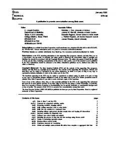
A Brief Background on Bland-Altman Plots For readers who are unfamiliar with the method, this section contains a brief description of Bland-Altman plots, as background. Figure 1 shows the principles of the method, using the data originally provided and analysed by Bland and Altman (1986)2. The data are Peak Expiratory Flow Rate (PEFR) measurements made with a Wright peak flow meter, and also with a Mini Wright peak flow meter on 17 patients (n=17). The typical Bland-Altman analysis shown in Figure 1 has the difference d between the two meters (Wright- Mini Wright) plotted on the y-axis

and the mean xave of the two measurements plotted on the x-axis. A horizontal reference line

� = -2.1 liters/minute) is typically included on showing the mean of the differences (in this case d

Bland-Altman plots. For the data in Figure 1, the standard deviation of the differences sdiff was 38.8 liters/minute.

Bland-Altman plots usually also include horizontal lines to denote 95% Limits of Agreement (LoAs). If the data were distributed normally and sample sizes were very large, one would expect approximately 95% of the differences (d) in the sample to lie within 1.96 standard

� . Thus the upper LoA is given by: deviations (i.e. 1.96 sdiff ) from the mean of differences d

� +1.96 sdiff Upper LoA=d

which in this example =−2.1 + 1.96x38.8 = 73.9 liters/minute. The lower LoA is given by: � -1.96 sdiff Lower LoA=d

which in this example =−2.1 − 1.96x38.8 = -78.1 liters/minute.

These LoAs, as shown in Figure 1, are actually slightly different from those shown in Bland and Altman (1986)2, because they used the slightly more conservative, and easier to calculate, LoAs � ± 1.96 sdiff. � ± 2 sdiff . Most authors currently use the more precise definition: d of d The mean of differences 𝑑̅ and LoAs are statistics that describe characteristics of the data

sample itself. However, for many cases, researchers and readers are concerned with how these statistics describe the population from which the sample is drawn.21 This can be done by using the information in the sample to estimate confidence intervals for a given parameter. Confidence intervals describe the range over which a parameter is likely to lie with a given probability, often 95%.

It is very common practice to calculate 95% confidence intervals for a mean such as 𝑑̅. This is

accomplished, assuming a normal distribution of data, using the standard error of the mean and the t-distribution, using the equation:

𝑠 𝑑̅ ± 𝑡0.975,𝑛−1 𝑑𝑖𝑓𝑓 . 𝑛 √

For the data in Figure 1, the critical t value for 16 degrees of freedom is 2.12. This gives a confidence interval from -22.0 to 17.8 liters/minute, indicated by error bars on the 𝑑̅ line in

Figure 1. In other words, it can be said that there is a 95% probability that the population mean 𝜇𝑑 for d values lies between -22.0 and 17.8 liters/minute. It is also possible to calculate 95% confidence intervals for LoAs, using the assumption that the data are distributed normally. Bland and Altman2, 6 described an approximate method for estimating such confidence limits and an example is shown as error bars on the LoAs in Figure 1. This approximation is based on the assumption that underlying differences d are distributed normally and that the variance of the difference is independent of the difference itself, and on

the assumption that the sample size is large. It is possible, using these assumptions, to approximate the standard error for an individual LoA as √3

√2.92

𝑠𝑑𝑖𝑓𝑓 6 . √𝑛

𝑠𝑑𝑖𝑓𝑓 2 or √𝑛

more precisely as

The approximation assumes that the probability density function for 𝜎𝑑𝑖𝑓𝑓 is normally

distributed, and that the probability density function for 𝑑̅ + 1.96 𝜎𝑑𝑖𝑓𝑓 is distributed as a t

distribution. These assumptions are approximately true for large values of n. The equations for confidence intervals by this approximate method from Bland and Altman(1999)6 are: Upper LoA±𝑡0.975,𝑛−1 √2.92 Lower LoA±𝑡0.975,𝑛−1 √2.92

𝑠𝑑𝑖𝑓𝑓 √𝑛

𝑠𝑑𝑖𝑓𝑓 √𝑛

In Figure 1 these give approximate 95% confidence intervals, symmetrically distributed around the LoAs, ranging from 39.8 to 108.0 liters/minute for the upper LoA and for the lower LoA, between -44.0 and -112.2 liters/minute.

Exact confidence Intervals for Upper or Lower LoAs Considered Individually Bland and Altman’s approximate method is derived using an implicit assumption that one is calculating a confidence interval for either the upper LoA or the lower LoA, but not both at the same time (i.e. LoAs considered individually). Owen 20 described the problem (for the upper LoA) as: Given a sample estimate of the mean (in this case 𝑑̅) and a sample estimate of the

standard deviation (in this case 𝑠𝑑𝑖𝑓𝑓 ) what value of k fills the criterion that a minimum

proportion, P, of the population is less than 𝑑̅ + 𝑘𝑠𝑑𝑖𝑓𝑓 with a confidence 𝛾? For Bland-Altman

95% LoAs, P=0.975 (corresponding to a Z score of 1.96) and for two-tailed 95% confidence

limits, k values are determined for 𝛾 = 0.025 and 𝛾 = 0.975. The same k values could also be used to determine 95% confidence limits for the lower LoA as 𝑑̅ − 𝑘𝑠𝑑𝑖𝑓𝑓 . Even though this is

typically determining two-tailed confidence limits, formally this process is known as determining

“one sided tolerance factors for a normal distribution” 20, because only one LoA is being considered at a time (either the upper or lower LoA). For Bland and Altman’s approximation: k≅ 1.96+ 𝑡0.975,𝑛−1

√2.92 √𝑛

and k≅ 1.96 - 𝑡0.975,𝑛−1

for 𝛾 = 0.975

√2.92 √𝑛

for 𝛾 = 0.025.

As stated above, Bland and Altman’s method may be inaccurate if n is not large. In fact, there are closer, but numerically more complicated approximations than Bland and Altman’s, which can be used for determining confidence limits for LoAs considered individually (e.g. the Method of Variance Estimates Recovery (MOVER).14,15

However, such approximations may be unnecessary, because the exact 95% confidence intervals for LoAs (considered individually) can be exactly estimated, for any sample size, large or small, assuming a normal distribution of the population from which 𝑑 is drawn. Using Owen’s20 equations, k can be determined for a P value of 0.975 using a non-central-t distribution. For different values of 𝛾, appropriate critical values are equal to 𝑘 where: 𝑃𝑟��𝑛𝑜𝑛𝑐𝑒𝑛𝑡𝑟𝑎𝑙 𝑡 𝑤𝑖𝑡ℎ 𝛿 = 𝑍0.975 √𝑛� ≤ 𝑘√𝑛� = 𝛾

As an aid for researchers, coefficients 𝑐0.025 and 𝑐0.975 have been calculated as k values

corresponding to 𝛾 values of 0.025 and 0.975. These coefficients are included in Table 1 for different degrees of freedom 𝜐 = 𝑛 − 1. Table 1 also includes 𝑐0.05 and 𝑐0.95 which could be

used to compute 2-tailed 90% confidence limits or 1-tailed 95% confidence limits and also 𝑐0.5

which may be used for determining median values for the confidence interval. The values have been computed to finer than the 10th decimal place using MATLAB and rounded to 4 decimal places in the table. Table 1 is abridged, but a more complete set of tables is available as a supplementary file (Appendix table 1, available at [LWW insert link]). Similar tables have been published to 3 decimal places by Odeh and Owen18 and in part, with small inaccuracies, by Owen20. As a further aid to researchers a supplementary file contains MATLAB code for

calculating coefficients found in Table 1. (MATLAB Kcalculator code, available at [LWW insert link]).

The exact and approximate confidence intervals differ for small subject numbers. To show this, the probability density function for the exact confidence interval for LoAs (considered individually) is shown in Figure 2B, along with the probability density function for the approximate method (Figure 2A), assuming n=5 (or degrees of freedom 𝜐 = 4 ) and given 𝑑̅ = 0

and 𝑠𝑑𝑖𝑓𝑓 = 1. The 1.96 line in Figure 2 shows the limit of agreement.

By way of example, exact confidence intervals for 95% LoAs, considered individually, are shown in Figure 1, calculated as follows. For the upper LoA, exact 95% confidence intervals are given by 𝑑̅ +𝑐0.025 𝑠𝑑𝑖𝑓𝑓 and 𝑑̅+𝑐0.975 𝑠𝑑𝑖𝑓𝑓 .

For the lower LoA, exact 95% confidence intervals are given by 𝑑̅-𝑐0.025 𝑠𝑑𝑖𝑓𝑓 and 𝑑̅-𝑐0.975 𝑠𝑑𝑖𝑓𝑓 .

From Table 1, for 16 degrees of freedom, 𝑐0.025 = 1.3150 and 𝑐0.975 = 3.1483. So, in Figure 1, for the upper LoA, 95% confidence intervals are bounded by −2.1 + 1.3150 × 38.8 =

48.9 liters/minute and −2.1 + 3.1483 × 38.8 = 120.0 liters/minute. For the lower LoA, 95%

intervals are bounded by −2.1 − 1.3150 × 38.8 = −53.1 liters/minute and −2.1 − 3.1483 × 38.8 = −124.2 liters/minute.

Figures 1 and 2 illustrate a number of general differences between the two methods for calculating LoA confidence intervals (considered individually). Firstly, exact confidence limits will be asymmetric about the LoAs, in contrast to the symmetry of Bland and Altman’s approximate method. The inner bound for the exact 95% confidence interval will always be closer to the LoA (and smaller than the approximate inner confidence interval) than the outer bound (which will

always be larger than the corresponding approximate confidence interval). However, this asymmetry becomes smaller as sample size increases. As a guide, for LoAs considered individually, the difference between exact and approximate 95% inner confidence limits becomes less than 0.1 𝑠𝑑𝑖𝑓𝑓 when degrees of freedom become greater than 37. The difference

between exact and approximate 95% outer confidence limits becomes less than 0.1 𝑠𝑑𝑖𝑓𝑓 when degrees of freedom become greater than 44.

In addition, the total magnitude of the approximate 95% confidence interval (the difference between inner and outer bounds) is always slightly smaller than the total magnitude of the exact confidence interval. This difference in total magnitude becomes smaller as n increases, being less than 0.1 sdiff for degrees of freedom greater than 13. Exact Confidence Intervals for Upper and Lower LoAs Considered as a Pair Bland-Altman LoAs are usually considered as a pair of bounds, and so it may be more appropriate for many applications to treat them as a pair when calculating their confidence limits. However, the methods demonstrated so far in this paper only estimate confidence intervals for LoAs considered individually. However, there are methods in which the confidence intervals are obtained for the LoAs considered as a pair. These arise from the literature on what is formally known as “two-sided tolerance factors for a normal distribution.” The problem can be stated as: given a sample estimate of the mean (in this case 𝑑̅) and a sample estimate of the standard deviation (in this case 𝑠𝑑𝑖𝑓𝑓 ) what value of 𝑘𝑡 fills the criterion that a minimum proportion, P, of the population lies between 𝑑̅ ± 𝑘𝑡 𝑠𝑑𝑖𝑓𝑓 with confidence 𝛾.20

Ludbrook13 was the first to apply this two-sided tolerance factors approach to the problem of calculating confidence limits for Bland-Altman LoAs. He used existing tables22 to provide an

upper 95% confidence limit (i.e. a one-tailed bound) for LoAs considered as a pair. These tables contained approximate coefficients, being reproductions of tables from Bowker23 published in 1947. The coefficients in Bowker’s tables were calculated using approximate methods described by Wald and Wolfowitz19. However, for values of 𝛾, the coefficients 𝑘𝑡 can be calculated exactly

by determining the value of 𝑘𝑡 which satisfies the equation 2√𝑛

√2𝜋

∞

� P(𝛾, 𝑘𝑡 |𝑥̅ ) 𝑒 − 0

1� 𝑛𝑥̅ 2 2 𝑑𝑥̅

=𝛾

2

Where P(𝛾, 𝑘𝑡 |𝑥̅ ) = 𝑃𝑟 �𝜒 2 > 𝜈𝑟 � 2 � 𝑘𝑡 And r is the root of the equation. 𝑥̅ +𝑟

𝑃=�

𝑥̅ −𝑟

𝜙(𝑡)𝑑𝑡

Where is 𝜙(𝑡) the standard normal probability density function.17, 24 Table 2 contains coefficients calculated by the author with MATLAB, using these equations and the method described by Odeh.17 Degrees of freedom have been defined as 𝜐 = 𝑛 − 1. Values

for 𝑘𝑡 , rounded to 4 decimal places, were calculated for P=0.95 by iterative methods for 𝛾 values

accurate to within 8 decimal places. Coefficients 𝑐𝑡 0.025 , 𝑐𝑡 0.05, 𝑐𝑡 0.5 , 𝑐𝑡 0.95 , 𝑐𝑡 0.975 are the 𝑘𝑡 values corresponding to 𝛾 values of 0.025, 0.05, 0.50, 0.95 and 0.975. Similar tables have

previously been published for exact 𝑐𝑡 0.5, 𝑐𝑡 0.95 and 𝑐𝑡 0.975 to 3 decimal places17, 18, and also for approximate19 𝑐𝑡 0.95values to 3 decimal places.23 Table 2 is abridged, but a more complete set

of tables is available as a supplementary file (Appendix table 2, available at [LWW insert link]).

As a further aid to researchers a supplementary file contains MATLAB code for calculating coefficients found in Table 2. (MATLAB Ktcalculator code, available at [LWW insert link]).

The above equations have also been used to derive Figure 2c, which shows the probability density functions for LoAs considered as a pair given 𝑑̅ = 0 and 𝑠𝑑𝑖𝑓𝑓 = 1, assuming n=5 (or

degrees of freedom 𝜐 = 4).

This approach of calculating confidence limits for LoAs considered as a pair is probably most suitable, in general, for determining confidence intervals for Bland-Altman LoAs. Confidence limits can be given by 𝑑̅ ± 𝑐𝑡 0.025 𝑠𝑑𝑖𝑓𝑓 and 𝑑̅ ± 𝑐𝑡 0.975 𝑠𝑑𝑖𝑓𝑓 . Using the data in Figure 1 as an example, with 𝜈 = 16 one can calculate a 2.5% lower bound

using the 𝑐𝑡 0.025 coefficient 1.4900 to determine there is a 2.5% probability that at least 95% of

the differences in the population lie between the bounds of −2.1 ± 1.4900 × 38.8 liters/minute, i.e. −2.1 ± 57.8 liters/minute. One could also calculate a 97.5% upper bound using the

𝑐𝑡 0.975 coefficient 3.0824 to determine there is a probability of 97.5% that at least 95% of the

differences in the population lie between the bounds of −2.1 ± 3.0824 × 38.8 liters/minute i.e.

−2.1 ± 119.6 liters/minute. Thus there is a 95% probability that at least 95% of the differences

in the population lie outside the limits of −2.1 ± 57.8 liters/minute (-59.9 and 55.7 liters/minute) and inside the limits of −2.1 ± 119.6 liters/minute (-121.7 and 117.5 liters/minute). These confidence limits have been included as a pair of error bars on the LoAs in Figure 1.

Figures 1 and 2 show subtle differences between exact confidence intervals for LoAs considered individually and as a pair. These differences are also apparent when comparing Table 1 and Table 2.

The exact confidence intervals for LoAs, considered as a pair, will also differ from those obtained by Bland and Altman’s approximate method, but the difference depends on sample size. The sample size at which this difference is acceptable, and at which the methods become interchangeable, will be a matter of judgement for researchers. As a guide, however: for LoAs considered as a pair, the difference between exact 95% inner confidence limits and Bland and Altman’s approximation becomes less than 0.1 𝑠𝑑𝑖𝑓𝑓 when degrees of freedom become greater

than 112. The difference between exact and approximate 95% outer confidence limits becomes less than 0.1 𝑠𝑑𝑖𝑓𝑓 when degrees of freedom become greater than 26. In addition, the total

magnitude of the approximate 95% confidence interval (the difference between inner and outer bounds) is smaller than the total magnitude of the exact confidence intervals, for degrees of freedom less than 8, and is larger for all other degrees of freedom. This absolute difference in total magnitude is less than 0.1 sdiff for degrees of freedom of 7, 8 and 9 and for degrees of

freedom greater than 150.

DISCUSSION It is good practice to calculate confidence intervals for Bland-Altman LoAs, especially if the sample size is small. The LoA calculated for a sample is only an estimate of the LoA for the population from which the sample is drawn and it is useful for researchers and readers to have an understanding of how much the LoAs in the population may vary from the sample LoAs.

This paper has described a number of approaches to calculating confidence intervals for BlandAltman LoAs, and the method chosen by researchers will depend, to some extent, on what aspects of the data the researchers wish to highlight.

Occasionally researchers might adopt an approach of determining confidence intervals for LoAs considered individually where they are especially concerned with inferences about either the top or bottom of the range of differences. An example might be comparing a new technique of tonometry with a pre-existing standard such as Goldmann tonometry and considering the range over which the new technique underestimates Goldmann pressures (and as a consequence there may be a chance of missing elevated IOP). In such situations the coefficients contained in Table 1 may be useful.

However, for most applications researchers will be concerned about both upper and lower LoAs and under these circumstances it is more appropriate to calculate the confidence limits for LoAs considered as a pair. This approach may fit best with the underlying principles of Bland-Altman analysis which generally involves determining a pair of LoAs. To illustrate where such calculations are useful, confidence intervals have been calculated for Bland-Altman limits of agreement for some previously published data sets.

The first comes from a recent study by Bandlitz et al 25 of techniques for measuring tear meniscus radius with a newly developed technique: PDM and with an existing technique VM. Figure 3 shows a Bland-Altman plot comparing in vitro radius measurements taken from 5 glass capillary tubes using the different instruments. The figure is as originally published, with the addition of confidence intervals calculated using coefficients from Table 2, plotted as error bars on the LoAs. The sample size (n=5) is relatively small to base the estimate of LoAs on, and calculating confidence intervals for LoAs may be useful under such circumstances. The mean of differences was 0.0002 mm with an estimated SD diff of 0.0205 mm. LoAs are shown at 0.0404 mm (confidence interval +0.0256 mm to 0.1264mm) and -0.0400 mm (confidence interval 0.0252 mm to -0.1260 mm). One could say, based on this sample, with 95% confidence, that in the population the LoAs could have been as wide apart as +0.1264 and -0.1260 mm, or as

close together as +0.0256 and -0.0252 mm. The authors made no comment interpreting the LoAs, beyond presenting the data, but if they had included the confidence intervals, readers would have seen that LoAs in the population are reasonably likely to lie considerably further from the mean of differences. A range of +/- 0.126 mm may still be acceptable LoAs in the science of meniscometry, but it is useful for readers to know the range when interpreting the research.

Figure 4 shows Bland-Altman plots, taken from a recent study of retinal oxygen saturation measurements obtained from specialized fundus imaging in 18 subjects.26 The figure shows intra-session variability in the measurements from retinal arteries in frame A, and retinal veins in frame B. The error bars were not in the original figure, but have been included to show the confidence limits for LoAs using the exact method and Table 2. Means of differences were 0.3% (with SD diff of 5.0%) for arteries and -0.6% (with SD diff of 8.0%) for veins. LoAs (with 95% confidence intervals) were 10.1% (7.8% to 15.5%) and -9.6% (-7.2% to -14.9%) for arteries and 15.0% (11.4% to 23.6%) and -16.2% (-12.6% to -24.8%) for veins.

In the original paper, the discussion section makes the observation that: “Furthermore, our analysis showed for the first time that there was no bias between (or within) recording sessions and that 95% LoAs are generally lower in arteries.” (Italics added.) There is not, currently, an appropriate inferential statistic to determine the specific question of whether the LoAs differ from one data set to another, (although a number of tests have been developed to assess the simpler question of whether variance is different between two samples27), but some guidance may be obtained from the confidence intervals. On the basis of the presented data, a claim that LoAs are different (for arteries and veins) is difficult to sustain, because of the overlap between the confidence intervals.

This is in contrast to the next example, a pediatric ocular biometry report12, in which the repeatability of ultrasound measurements (Echoscan) of axial lengths in children were compared with partial coherence interferometry measurements (IOLmaster) of axial length. This is shown as repeatability Bland–Altman plots in Figure 5, as originally published, except for the addition of confidence intervals (again calculated from Table 2) for LoAs drawn as error bars. For 37 subjects, 2 measurements were repeated with each instrument. The IOLmaster tends to give quite repeatable results with a lower LoA of -0.05mm (with a CI of between -0.04 mm and 0.06 mm) and an upper LoA of +0.04mm (with a CI of between 0.03 mm and 0.05 mm). Echoscan gives less repeatable results. The mean of differences was -0.094 mm and the SD diff was 0.388 mm. The lower LoA was -0.85 mm (with a CI of between -0.71 mm and -1.09 mm). The upper LoA was 0.67mm (with a CI of between 0.53 mm and 0.91 mm). In this case, the addition of confidence intervals supports the initial paper’s inference that IOLmaster had better repeatability than Echoscan measurements of axial length because the outer 95% confidence intervals for the IOLmaster LoAs lie well inside the inner 95% confidence intervals for Echoscan LoAs. In addition the confidence intervals may help readers in planning future research, or making comparisons with other studies, because they provide estimates for where the LoAs might be expected to lie in the population.

CONCLUSIONS This paper has described exact parametric methods for determining confidence intervals for LoAs. As an application to Bland-Altman analysis the methods have only been partially described before using approximate coefficients13, although the numerical techniques are well established. 17, 18, 20 This exact parametric method may be best but even an approximate calculation of confidence intervals for LoAs is likely to be better than none at all.

Researchers may find the new technique useful, especially for small sample sizes. Whether they decide to use confidence limits for LoAs either considered as a pair or considered individually, or exact or approximate methods, authors should always describe the method used for their calculations. In addition, authors should recognize that readers may wish to consider alternative inferences from their data. By reporting 𝑑̅, 𝑠𝑑𝑖𝑓𝑓 and n values, authors will give

readers the information that can be used for alternative calculations of confidence intervals for LoAs.

Finally, authors should consider whether it is useful to include a set of error bars in their BlandAltman plots, to show confidence intervals for LoAs as in Figures 1,3,4 and 5, or merely to report the confidence intervals as values. While they are a convenient way to show the confidence intervals, error bars themselves can be interpreted in a number of different ways, e.g., representing standard deviations or standard errors. Authors should take care to explain in figure legends what the error bars represent and the method used for calculating them.

APPENDIX/SUPPLEMENTAL DIGITAL CONTENT Appendix table 1, listing coefficients for calculating exact 95% confidence intervals for 95% LoAs considered individually, for different degrees of freedom 𝜐 = 𝑛 − 1, is available at [LWW

insert link]. Appendix table 2, listing coefficients for calculating exact 95% confidence intervals for 95% LoAs considered as a pair, for different degrees of freedom 𝜐 = 𝑛 − 1, is available at

[LWW insert link]. MATLAB Kcalculator code, for calculating coefficient values in Table 1 and Appendix table 1 is available at [LWW insert link]. MATLAB Ktcalculator code, for calculating coefficient values in Table 2 and Appendix table 2 is available at [LWW insert link].

REFERENCES 1.

Altman DG, Bland JM. Measurement in medicine: the analysis of method comparison studies. The Statistician 1983;32:307-17.

2.

Bland JM, Altman DG. Statistical methods for assessing agreement between two methods of clinical measurement. Lancet 1986;327:307-10.

3.

Web of Science [Available at: http://apps.webofknowledge.com.ezp01.library.qut.edu.au/full_record.do?product=WOS&s earch_mode=GeneralSearch&qid=5&SID=P14JIkE7fBrFN83KsWh&page=1&doc=3. Accessed: 3/09/2014];

4.

Mantha R, Roizen MF, Fleisher LA, Thisted R, J. F. Comparing methods of clinical measurement: Reporting standards for Bland and Altman analysis. Anesth Analg 2000;90:593-602.

5.

Armstrong RA, Davies LN, Dunne MCM, Gilmartin B. Statistical guidelines for clinical studies of human vision. Ophthal Physiol Opt 2011;31:123-36.

6.

Bland JM, Altman DG. Measuring agreement in method comparison studies. Stat Methods Med Res 1999;8:135-60.

7.

McAlinden C, Khadka J, Pesudovs K. Statistical methods for conducting agreement (comparison of clinical tests) and precision (repeatability or reproducibility) studies in optometry and ophthalmology. Ophthal Physiol Opt 2011;31:330-8.

8.

Ophthalmic and Physiological Optics, author guidelines.; [Available at: http://onlinelibrary.wiley.com/journal/10.1111/(ISSN)14751313/homepage/ForAuthors.html. Accessed: 12/09/2014];

9.

McAlinden C, Khadka J, Pesudovs K. Agreement studies: clarification. Ophthal Physiol Opt 2012;32:439-40.

10. Hamilton C, Stamey J. Using Bland-Altman to assess agreement between two medical devices - Don't forget the confidence intervals! J Clin Monitor Comp 2007;21:331-3. . 11. McClenaghan N, Kimura A, Stark LR. An evaluation of the M&S Technologies Smart System II for visual acuity measurement in young visually-normal adults. Optom Vis Sci 2007;84:218-23. 12. Carkeet A, Saw SM, Gazzard G, Tang W, Tan DT. Repeatability of IOLMaster biometry in children. Optom Vis Sci 2004;81:829-34. 13. Ludbrook J. Confidence in Altman-Bland plots: a critical review of the method of differences. Clin Exp Pharmacol Physiol 2010;37:143-9. 14. Donner A, Zou GY. Closed-form confidence intervals for functions of the normal mean and standard deviation. Stat Methods Med Res 2010;21:347–59. 15. Zou GY. Confidence interval estimation for the Bland-Altman limits of agreement with multiple observations per individual. Stat Methods Med Res 2013;22:630-42. 16. Olofsen E, Dahan A, Borsboom G, Drummond G. Improvements in the application and reporting of advanced Bland-Altman methods of comparison. J Clin Monit Comput 2014:Epub 8 May, 2014. 17. Odeh RE. Tables of two-sided tolerance factors for a normal distribution. Commun Stat Simulat 1978;7:183-201. 18. Odeh RE, Owen DB. Tables for Normal Tolerance Limits, Sampling Plans, and Screening. New York Marcel Dekker, Inc; 1980.

19. Wald A, Wolfowitz J. Tolerance limits for a normal distribution. Ann Math Stat 1946;17:208-15. 20. Owen DB. Handbook of Statistical Tables: Addison-Wesley, Reading Massachusetts; 1962. 21. Gardner MJ, Altman DG. Estimating with confidence. Br Med J 1988;296:1210-1. 22. Lentner C, editor. Introduction to Statistics, Statistical tables, Mathematical Formulae. Basle: Ciba-Geigy Limited,; 1982. 23. Bowker AH. Tolerance Limits for Normal Distributions. In: Eisenhart C, Hastay MW, Wallis WA, ed. Selected Techniques of Statistical Analysis for Scientific and Industrial Research Production and Management Engineering New York: McGraw-Hill Book Company, 1947: 97-110. 24. Eberhardt KR, Mee RW, C.P. R. Computing factors for exact two-sided tolerance limits for a normal distribution. Commun Stat Simulat 1989;18:397-413. 25. Bandlitz S, Purslow C, Murphy PJ, Pult H, Bron AJ. A new portable digital meniscometer. Optom Vis Sci 2014;91:e1-e8. 26. O'Connell RA, Anderson AJ, Hosking SL, Batcha AH, Bui BV. Test-retest reliability of retinal oxygen saturation measurement. Optom Vis Sci 2014;91:608-14. 27. Brown MB, Forsythe AB. Robust tests for the equality of variances. J Am Stat Assoc 1974;69:364-7. Correspondence to: Andrew Carkeet School of Optometry and Vision Science QUT, GPO Box 2434 Brisbane Qld 4001 AUSTRALIA e-mail: [email protected]

Table 1. Coefficients for calculating exact 95% confidence intervals for 95% LoAs considered individually, for different degrees of freedom 𝜐 = 𝑛 − 1. (This table is abridged. A more complete table is attached as Appendix table 1, available at [LWW insert link]. 𝝂

1 2 3 4 5 6 7 8 9 10 11 12 13 14 15 16 17 18 19 20 25 30 35 36 40 50 60 70 80 90 100 120 140 160 180 200 250 300 350 400 450 500 1000

𝒄𝟎.𝟎𝟐𝟓

0.5226 0.7126 0.8349 0.9232 0.9912 1.0459 1.0913 1.1299 1.1632 1.1924 1.2183 1.2415 1.2625 1.2815 1.2990 1.3150 1.3299 1.3436 1.3565 1.3685 1.4187 1.4574 1.4883 1.4938 1.5139 1.5542 1.5848 1.6092 1.6292 1.6460 1.6604 1.6840 1.7026 1.7178 1.7305 1.7414 1.7628 1.7789 1.7915 1.8018 1.8104 1.8177 1.8578

𝒄𝟎.𝟎𝟓

0.7109 0.8748 0.9825 1.0606 1.1208 1.1693 1.2094 1.2434 1.2728 1.2986 1.3214 1.3418 1.3602 1.3769 1.3922 1.4063 1.4193 1.4313 1.4426 1.4530 1.4969 1.5305 1.5574 1.5621 1.5795 1.6144 1.6408 1.6618 1.6790 1.6934 1.7058 1.7260 1.7419 1.7549 1.7657 1.7750 1.7933 1.8070 1.8177 1.8265 1.8337 1.8399 1.8739

𝒄𝟎.𝟓𝟎

2.8197 2.3205 2.1862 2.1244 2.0891 2.0662 2.0502 2.0384 2.0293 2.0221 2.0162 2.0114 2.0073 2.0038 2.0008 1.9982 1.9959 1.9939 1.9921 1.9904 1.9842 1.9801 1.9772 1.9767 1.9750 1.9720 1.9700 1.9685 1.9675 1.9666 1.9660 1.9650 1.9642 1.9637 1.9633 1.9630 1.9624 1.9620 1.9617 1.9615 1.9613 1.9612 1.9606

𝒄𝟎.𝟗𝟓

31.2575 8.9861 6.0150 4.9085 4.3291 3.9696 3.7228 3.5417 3.4025 3.2915 3.2007 3.1248 3.0603 3.0046 2.9559 2.9130 2.8748 2.8405 2.8095 2.7814 2.6716 2.5949 2.5376 2.5278 2.4929 2.4268 2.3797 2.3441 2.3160 2.2931 2.2740 2.2438 2.2207 2.2023 2.1873 2.1747 2.1504 2.1327 2.1192 2.1083 2.0994 2.0919 2.0519

𝒄𝟎.𝟗𝟕𝟓

62.5576 12.8162 7.7095 5.9749 5.1109 4.5916 4.2432 3.9918 3.8009 3.6505 3.5285 3.4272 3.3416 3.2682 3.2044 3.1483 3.0985 3.0541 3.0140 2.9777 2.8370 2.7395 2.6672 2.6549 2.6111 2.5285 2.4701 2.4260 2.3913 2.3632 2.3397 2.3026 2.2744 2.2520 2.2337 2.2184 2.1889 2.1675 2.1510 2.1379 2.1272 2.1181 2.0700

Table 2. Coefficients for calculating exact 95% confidence intervals for 95% LoAs considered as a pair, for different degrees of freedom 𝜐 = 𝑛 − 1. (This table is abridged. A more complete table is attached as Appendix table 2, available at [LWW insert link]. 𝝂

1 2 3 4 5 6 7 8 9 10 11 12 13 14 15 16 17 18 19 20 25 30 35 36 40 50 60 70 80 90 100 120 140 160 180 200 250 300 350 400 450 500 1000

𝒄𝒕 𝟎.𝟎𝟐𝟓

0.9744 1.1051 1.1839 1.2397 1.2825 1.3170 1.3457 1.3702 1.3915 1.4102 1.4269 1.4419 1.4555 1.4680 1.4794 1.4900 1.4998 1.5089 1.5175 1.5255 1.5593 1.5856 1.6070 1.6108 1.6247 1.6530 1.6747 1.6922 1.7066 1.7188 1.7293 1.7466 1.7603 1.7716 1.7811 1.7893 1.8055 1.8177 1.8273 1.8352 1.8418 1.8474 1.8786

𝒄𝒕 𝟎.𝟎𝟓

1.1237 1.2333 1.3004 1.3481 1.3847 1.4142 1.4387 1.4596 1.4778 1.4938 1.5081 1.5209 1.5325 1.5431 1.5529 1.5619 1.5703 1.5780 1.5853 1.5922 1.6210 1.6434 1.6615 1.6647 1.6766 1.7006 1.7191 1.7339 1.7461 1.7564 1.7653 1.7800 1.7916 1.8012 1.8092 1.8161 1.8298 1.8401 1.8483 1.8549 1.8605 1.8652 1.8915

𝒄𝒕 𝟎.𝟓𝟎

3.3756 2.6342 2.4157 2.3080 2.2428 2.1988 2.1670 2.1429 2.1239 2.1085 2.0958 2.0852 2.0761 2.0682 2.0614 2.0554 2.0501 2.0453 2.0410 2.0371 2.0223 2.0122 2.0050 2.0038 1.9995 1.9918 1.9866 1.9829 1.9800 1.9778 1.9761 1.9734 1.9715 1.9701 1.9690 1.9681 1.9665 1.9654 1.9646 1.9640 1.9636 1.9632 1.9616

𝒄𝒕 𝟎.𝟗𝟓

36.5192 9.7888 6.3411 5.0769 4.4222 4.0196 3.7455 3.5459 3.3934 3.2728 3.1747 3.0931 3.0241 2.9649 2.9135 2.8683 2.8283 2.7925 2.7603 2.7312 2.6187 2.5414 2.4844 2.4747 2.4404 2.3762 2.3312 2.2975 2.2712 2.2499 2.2323 2.2046 2.1836 2.1671 2.1536 2.1424 2.1210 2.1055 2.0937 2.0843 2.0766 2.0701 2.0361

𝒄𝒕 𝟎.𝟗𝟕𝟓

73.0772 13.9396 8.1045 6.1569 5.1983 4.6276 4.2478 3.9757 3.7706 3.6100 3.4805 3.3736 3.2837 3.2069 3.1405 3.0824 3.0311 2.9854 2.9445 2.9075 2.7654 2.6685 2.5975 2.5855 2.5429 2.4637 2.4084 2.3671 2.3350 2.3090 2.2876 2.2539 2.2286 2.2085 2.1923 2.1788 2.1529 2.1342 2.1200 2.1087 2.0994 2.0917 2.0509

FIGURE LEGENDS Figure 1. Bland-Altman plot comparing 2 methods of measuring Peak Expiratory Flow, data taken from Bland and Altman’s 1986 paper.2 Error bars represent 95% confidence limits calculated by different methods, as indicated. Figure 2. Probability density functions for confidence intervals for 95% LoAs (degrees of freedom 𝜐 = 4, 𝑑̅ = 0 and 𝑠𝑑𝑖𝑓𝑓 = 1). Shaded tails represent upper and lower 2.5% of the

confidence interval. The 1.96 line shows the Bland-Altman LoA. a.) Bland and Altman’s

approximate method for LoAs considered individually. b.) Exact method for LoAs considered individually. c.) Exact method for LoAs considered as a pair (upper LoA shown). Figure 3. Bland-Altman analysis for comparison of two tear meniscometry systems (PDM and VM). (Reproduced with permission from Bandlitz et al.25). Measurements were made on five different capillary tubes’ sections. The figure is as originally published except for the addition of error bars showing the confidence intervals for LoAs considered as a pair. Figure 4. Bland-Altman analysis for intrasession repeatability of retinal oxygen saturation measurements made on retinal arteries (A) and retinal veins (B), from a recent study (Reproduced with permission from O’Connell et al.26) The figure is as originally published except for the addition of error bars showing the confidence intervals for LoAs considered as a pair. Figure 5. Bland-Altman analyses for repeatability of axial length in 37 children. (Reproduced with permission from Carkeet et al.12) (left panel) IOLmaster measurements. (right panel) Echoscan measurements. The figure is as published originally, except that exact 95% confidence intervals for LoAs considered as a pair have been added (error bars). At this scale the IOLmaster confidence limits (indicated by arrow) abut the LoAs.

Figure 1.

Figure 2

Figure 3

Figure 4

Figure 5

Coefficients for calculating exact 95% confidence intervals for 95% LoAs considered individually, for different degrees of freedom 𝜐 = 𝑛 − 1. 𝝂 1 2 3 4 5 6 7 8 9 10 11 12 13 14 15 16 17 18 19 20 21 22 23 24 25 26 27 28 29 30 31 32 33 34 35 36 37 38 39 40 41 42 43 44 45 46 47 48 49 50 51 52 53 54 55 56 57 58 59 60 61 62 63 64 65 66 67 68 69 70 71 72 73

𝒄𝟎.𝟎𝟐𝟓 0.5226 0.7126 0.8349 0.9232 0.9912 1.0459 1.0913 1.1299 1.1632 1.1924 1.2183 1.2415 1.2625 1.2815 1.2990 1.3150 1.3299 1.3436 1.3565 1.3685 1.3798 1.3903 1.4003 1.4098 1.4187 1.4272 1.4353 1.4430 1.4503 1.4574 1.4641 1.4705 1.4767 1.4826 1.4883 1.4938 1.4991 1.5042 1.5092 1.5139 1.5186 1.5230 1.5273 1.5315 1.5356 1.5395 1.5434 1.5471 1.5507 1.5542 1.5576 1.5610 1.5642 1.5674 1.5705 1.5735 1.5764 1.5793 1.5821 1.5848 1.5875 1.5901 1.5927 1.5952 1.5977 1.6001 1.6024 1.6047 1.6070 1.6092 1.6114 1.6135 1.6156

𝒄𝟎.𝟎𝟓 0.7109 0.8748 0.9825 1.0606 1.1208 1.1693 1.2094 1.2434 1.2728 1.2986 1.3214 1.3418 1.3602 1.3769 1.3922 1.4063 1.4193 1.4313 1.4426 1.4530 1.4629 1.4721 1.4808 1.4891 1.4969 1.5042 1.5113 1.5180 1.5244 1.5305 1.5363 1.5419 1.5473 1.5524 1.5574 1.5621 1.5667 1.5711 1.5754 1.5795 1.5835 1.5874 1.5911 1.5948 1.5983 1.6017 1.6050 1.6082 1.6113 1.6144 1.6173 1.6202 1.6230 1.6257 1.6284 1.6310 1.6335 1.6360 1.6384 1.6408 1.6431 1.6454 1.6476 1.6497 1.6519 1.6539 1.6559 1.6579 1.6599 1.6618 1.6637 1.6655 1.6673

𝒄𝟎.𝟓𝟎 2.8197 2.3205 2.1862 2.1244 2.0891 2.0662 2.0502 2.0384 2.0293 2.0221 2.0162 2.0114 2.0073 2.0038 2.0008 1.9982 1.9959 1.9939 1.9921 1.9904 1.9889 1.9876 1.9864 1.9853 1.9842 1.9833 1.9824 1.9816 1.9808 1.9801 1.9795 1.9789 1.9783 1.9777 1.9772 1.9767 1.9763 1.9758 1.9754 1.9750 1.9747 1.9743 1.9740 1.9737 1.9734 1.9731 1.9728 1.9725 1.9723 1.9720 1.9718 1.9715 1.9713 1.9711 1.9709 1.9707 1.9705 1.9703 1.9702 1.9700 1.9698 1.9697 1.9695 1.9694 1.9692 1.9691 1.9689 1.9688 1.9687 1.9685 1.9684 1.9683 1.9682

𝒄𝟎.𝟗𝟓

31.2575 8.9861 6.0150 4.9085 4.3291 3.9696 3.7228 3.5417 3.4025 3.2915 3.2007 3.1248 3.0603 3.0046 2.9559 2.9130 2.8748 2.8405 2.8095 2.7814 2.7557 2.7321 2.7104 2.6903 2.6716 2.6542 2.6379 2.6227 2.6083 2.5949 2.5821 2.5701 2.5587 2.5479 2.5376 2.5278 2.5185 2.5095 2.5010 2.4929 2.4850 2.4775 2.4703 2.4634 2.4567 2.4503 2.4441 2.4381 2.4324 2.4268 2.4214 2.4162 2.4111 2.4062 2.4015 2.3969 2.3924 2.3881 2.3838 2.3797 2.3758 2.3719 2.3681 2.3644 2.3608 2.3573 2.3539 2.3506 2.3473 2.3441 2.3410 2.3380 2.3350

𝒄𝟎.𝟗𝟕𝟓 62.5576 12.8162 7.7095 5.9749 5.1109 4.5916 4.2432 3.9918 3.8009 3.6505 3.5285 3.4272 3.3416 3.2682 3.2044 3.1483 3.0985 3.0541 3.0140 2.9777 2.9447 2.9144 2.8865 2.8608 2.8370 2.8148 2.7941 2.7747 2.7566 2.7395 2.7234 2.7082 2.6938 2.6802 2.6672 2.6549 2.6432 2.6320 2.6213 2.6111 2.6013 2.5919 2.5829 2.5742 2.5659 2.5578 2.5501 2.5427 2.5355 2.5285 2.5218 2.5153 2.5090 2.5030 2.4971 2.4913 2.4858 2.4804 2.4752 2.4701 2.4651 2.4603 2.4556 2.4511 2.4466 2.4423 2.4381 2.4340 2.4299 2.4260 2.4222 2.4184 2.4148

Coefficients for CIs. LoAs considered individually. 𝝂

74 75 76 77 78 79 80 81 82 83 84 85 86 87 88 89 90 91 92 93 94 95 96 97 98 99 100 101 102 103 104 105 106 107 108 109 110 111 112 113 114 115 116 117 118 119 120 121 122 123 124 125 126 127 128 129 130 131 132 133 134 135 136 137 138 139 140 141 142 143 144 145 146 147 148 149 150 151 152 153

𝒄𝟎.𝟎𝟐𝟓 1.6177 1.6197 1.6216 1.6236 1.6255 1.6274 1.6292 1.6310 1.6328 1.6345 1.6363 1.6379 1.6396 1.6413 1.6429 1.6444 1.6460 1.6475 1.6491 1.6506 1.6520 1.6535 1.6549 1.6563 1.6577 1.6591 1.6604 1.6617 1.6631 1.6643 1.6656 1.6669 1.6681 1.6693 1.6706 1.6718 1.6729 1.6741 1.6752 1.6764 1.6775 1.6786 1.6797 1.6808 1.6819 1.6829 1.6840 1.6850 1.6860 1.6870 1.6880 1.6890 1.6900 1.6909 1.6919 1.6928 1.6938 1.6947 1.6956 1.6965 1.6974 1.6983 1.6992 1.7000 1.7009 1.7017 1.7026 1.7034 1.7042 1.7050 1.7058 1.7066 1.7074 1.7082 1.7090 1.7098 1.7105 1.7113 1.7120 1.7128

𝒄𝟎.𝟎𝟓 1.6690 1.6708 1.6725 1.6741 1.6758 1.6774 1.6790 1.6805 1.6821 1.6836 1.6850 1.6865 1.6879 1.6893 1.6907 1.6921 1.6934 1.6947 1.6960 1.6973 1.6986 1.6998 1.7010 1.7023 1.7034 1.7046 1.7058 1.7069 1.7080 1.7091 1.7102 1.7113 1.7124 1.7134 1.7145 1.7155 1.7165 1.7175 1.7185 1.7195 1.7204 1.7214 1.7223 1.7232 1.7242 1.7251 1.7260 1.7268 1.7277 1.7286 1.7294 1.7303 1.7311 1.7319 1.7327 1.7336 1.7344 1.7351 1.7359 1.7367 1.7375 1.7382 1.7390 1.7397 1.7404 1.7412 1.7419 1.7426 1.7433 1.7440 1.7447 1.7454 1.7460 1.7467 1.7474 1.7480 1.7487 1.7493 1.7500 1.7506

𝒄𝟎.𝟓𝟎 1.9681 1.9680 1.9679 1.9678 1.9677 1.9676 1.9675 1.9674 1.9673 1.9672 1.9671 1.9670 1.9669 1.9669 1.9668 1.9667 1.9666 1.9666 1.9665 1.9664 1.9663 1.9663 1.9662 1.9661 1.9661 1.9660 1.9660 1.9659 1.9658 1.9658 1.9657 1.9657 1.9656 1.9656 1.9655 1.9655 1.9654 1.9654 1.9653 1.9653 1.9652 1.9652 1.9651 1.9651 1.9650 1.9650 1.9650 1.9649 1.9649 1.9648 1.9648 1.9648 1.9647 1.9647 1.9646 1.9646 1.9646 1.9645 1.9645 1.9645 1.9644 1.9644 1.9644 1.9643 1.9643 1.9643 1.9642 1.9642 1.9642 1.9642 1.9641 1.9641 1.9641 1.9640 1.9640 1.9640 1.9640 1.9639 1.9639 1.9639

𝒄𝟎.𝟗𝟓 2.3322 2.3293 2.3265 2.3238 2.3212 2.3186 2.3160 2.3135 2.3111 2.3087 2.3063 2.3040 2.3018 2.2996 2.2974 2.2952 2.2931 2.2911 2.2890 2.2871 2.2851 2.2832 2.2813 2.2794 2.2776 2.2758 2.2740 2.2723 2.2706 2.2689 2.2672 2.2656 2.2640 2.2624 2.2609 2.2593 2.2578 2.2563 2.2548 2.2534 2.2520 2.2505 2.2492 2.2478 2.2464 2.2451 2.2438 2.2425 2.2412 2.2399 2.2387 2.2374 2.2362 2.2350 2.2338 2.2327 2.2315 2.2304 2.2292 2.2281 2.2270 2.2259 2.2249 2.2238 2.2227 2.2217 2.2207 2.2197 2.2187 2.2177 2.2167 2.2157 2.2147 2.2138 2.2129 2.2119 2.2110 2.2101 2.2092 2.2083

𝒄𝟎.𝟗𝟕𝟓 2.4112 2.4077 2.4043 2.4010 2.3977 2.3945 2.3913 2.3883 2.3852 2.3823 2.3794 2.3766 2.3738 2.3711 2.3684 2.3657 2.3632 2.3606 2.3581 2.3557 2.3533 2.3509 2.3486 2.3463 2.3441 2.3419 2.3397 2.3376 2.3355 2.3334 2.3314 2.3294 2.3274 2.3254 2.3235 2.3216 2.3198 2.3180 2.3162 2.3144 2.3126 2.3109 2.3092 2.3075 2.3059 2.3042 2.3026 2.3010 2.2995 2.2979 2.2964 2.2949 2.2934 2.2919 2.2905 2.2890 2.2876 2.2862 2.2848 2.2835 2.2821 2.2808 2.2795 2.2782 2.2769 2.2756 2.2744 2.2731 2.2719 2.2707 2.2695 2.2683 2.2672 2.2660 2.2648 2.2637 2.2626 2.2615 2.2604 2.2593


154 155 156 157 158 159 160 161 162 163 164 165 166 167 168 169 170 171 172 173 174 175 176 177 178 179 180 181 182 183 184 185 186 187 188 189 190 191 192 193 194 195 196 197 198 199 200 201 202 203 204 205 206 207 208 209 210 211 212 213 214 215 216 217 218 219 220 221 222 223 224 225 226 227 228 229 230 231 232 233

𝒄𝟎.𝟎𝟐𝟓 1.7135 1.7142 1.7150 1.7157 1.7164 1.7171 1.7178 1.7185 1.7191 1.7198 1.7205 1.7212 1.7218 1.7225 1.7231 1.7238 1.7244 1.7250 1.7257 1.7263 1.7269 1.7275 1.7281 1.7287 1.7293 1.7299 1.7305 1.7311 1.7317 1.7322 1.7328 1.7334 1.7339 1.7345 1.7350 1.7356 1.7361 1.7367 1.7372 1.7377 1.7383 1.7388 1.7393 1.7398 1.7403 1.7409 1.7414 1.7419 1.7424 1.7429 1.7434 1.7438 1.7443 1.7448 1.7453 1.7458 1.7462 1.7467 1.7472 1.7476 1.7481 1.7485 1.7490 1.7495 1.7499 1.7503 1.7508 1.7512 1.7517 1.7521 1.7525 1.7530 1.7534 1.7538 1.7542 1.7546 1.7550 1.7555 1.7559 1.7563

𝒄𝟎.𝟎𝟓 1.7512 1.7518 1.7525 1.7531 1.7537 1.7543 1.7549 1.7555 1.7560 1.7566 1.7572 1.7578 1.7583 1.7589 1.7594 1.7600 1.7605 1.7611 1.7616 1.7621 1.7627 1.7632 1.7637 1.7642 1.7647 1.7652 1.7657 1.7662 1.7667 1.7672 1.7677 1.7682 1.7687 1.7691 1.7696 1.7701 1.7705 1.7710 1.7715 1.7719 1.7724 1.7728 1.7733 1.7737 1.7741 1.7746 1.7750 1.7754 1.7759 1.7763 1.7767 1.7771 1.7775 1.7779 1.7784 1.7788 1.7792 1.7796 1.7800 1.7804 1.7807 1.7811 1.7815 1.7819 1.7823 1.7827 1.7830 1.7834 1.7838 1.7842 1.7845 1.7849 1.7852 1.7856 1.7860 1.7863 1.7867 1.7870 1.7874 1.7877

𝒄𝟎.𝟓𝟎 1.9639 1.9638 1.9638 1.9638 1.9638 1.9637 1.9637 1.9637 1.9637 1.9636 1.9636 1.9636 1.9636 1.9635 1.9635 1.9635 1.9635 1.9635 1.9634 1.9634 1.9634 1.9634 1.9634 1.9633 1.9633 1.9633 1.9633 1.9633 1.9633 1.9632 1.9632 1.9632 1.9632 1.9632 1.9631 1.9631 1.9631 1.9631 1.9631 1.9631 1.9630 1.9630 1.9630 1.9630 1.9630 1.9630 1.9630 1.9629 1.9629 1.9629 1.9629 1.9629 1.9629 1.9629 1.9628 1.9628 1.9628 1.9628 1.9628 1.9628 1.9628 1.9627 1.9627 1.9627 1.9627 1.9627 1.9627 1.9627 1.9627 1.9626 1.9626 1.9626 1.9626 1.9626 1.9626 1.9626 1.9626 1.9626 1.9625 1.9625

𝒄𝟎.𝟗𝟓 2.2074 2.2065 2.2057 2.2048 2.2040 2.2031 2.2023 2.2015 2.2007 2.1999 2.1991 2.1983 2.1975 2.1967 2.1960 2.1952 2.1944 2.1937 2.1930 2.1922 2.1915 2.1908 2.1901 2.1894 2.1887 2.1880 2.1873 2.1866 2.1859 2.1853 2.1846 2.1839 2.1833 2.1826 2.1820 2.1813 2.1807 2.1801 2.1795 2.1789 2.1782 2.1776 2.1770 2.1764 2.1758 2.1753 2.1747 2.1741 2.1735 2.1730 2.1724 2.1718 2.1713 2.1707 2.1702 2.1696 2.1691 2.1686 2.1680 2.1675 2.1670 2.1665 2.1660 2.1654 2.1649 2.1644 2.1639 2.1634 2.1629 2.1624 2.1620 2.1615 2.1610 2.1605 2.1600 2.1596 2.1591 2.1586 2.1582 2.1577

𝒄𝟎.𝟗𝟕𝟓 2.2582 2.2572 2.2561 2.2551 2.2540 2.2530 2.2520 2.2510 2.2500 2.2490 2.2480 2.2471 2.2461 2.2452 2.2442 2.2433 2.2424 2.2415 2.2406 2.2397 2.2388 2.2379 2.2371 2.2362 2.2354 2.2345 2.2337 2.2329 2.2320 2.2312 2.2304 2.2296 2.2288 2.2280 2.2272 2.2265 2.2257 2.2249 2.2242 2.2234 2.2227 2.2220 2.2212 2.2205 2.2198 2.2191 2.2184 2.2177 2.2170 2.2163 2.2156 2.2149 2.2142 2.2136 2.2129 2.2122 2.2116 2.2109 2.2103 2.2096 2.2090 2.2084 2.2078 2.2071 2.2065 2.2059 2.2053 2.2047 2.2041 2.2035 2.2029 2.2023 2.2017 2.2012 2.2006 2.2000 2.1994 2.1989 2.1983 2.1978


234 235 236 237 238 239 240 241 242 243 244 245 246 247 248 249 250 251 252 253 254 255 256 257 258 259 260 261 262 263 264 265 266 267 268 269 270 271 272 273 274 275 276 277 278 279 280 281 282 283 284 285 286 287 288 289 290 291 292 293 294 295 296 297 298 299 300 301 302 303 304 305 306 307 308 309 310 311 312 313

𝒄𝟎.𝟎𝟐𝟓 1.7567 1.7571 1.7575 1.7579 1.7583 1.7587 1.7591 1.7594 1.7598 1.7602 1.7606 1.7610 1.7614 1.7617 1.7621 1.7625 1.7628 1.7632 1.7636 1.7639 1.7643 1.7646 1.7650 1.7654 1.7657 1.7661 1.7664 1.7667 1.7671 1.7674 1.7678 1.7681 1.7684 1.7688 1.7691 1.7694 1.7698 1.7701 1.7704 1.7708 1.7711 1.7714 1.7717 1.7720 1.7724 1.7727 1.7730 1.7733 1.7736 1.7739 1.7742 1.7745 1.7748 1.7751 1.7754 1.7757 1.7760 1.7763 1.7766 1.7769 1.7772 1.7775 1.7778 1.7781 1.7783 1.7786 1.7789 1.7792 1.7795 1.7798 1.7800 1.7803 1.7806 1.7809 1.7811 1.7814 1.7817 1.7819 1.7822 1.7825

𝒄𝟎.𝟎𝟓 1.7881 1.7884 1.7887 1.7891 1.7894 1.7898 1.7901 1.7904 1.7907 1.7911 1.7914 1.7917 1.7920 1.7924 1.7927 1.7930 1.7933 1.7936 1.7939 1.7942 1.7945 1.7948 1.7951 1.7955 1.7957 1.7960 1.7963 1.7966 1.7969 1.7972 1.7975 1.7978 1.7981 1.7984 1.7987 1.7989 1.7992 1.7995 1.7998 1.8000 1.8003 1.8006 1.8009 1.8011 1.8014 1.8017 1.8019 1.8022 1.8025 1.8027 1.8030 1.8033 1.8035 1.8038 1.8040 1.8043 1.8045 1.8048 1.8050 1.8053 1.8055 1.8058 1.8060 1.8063 1.8065 1.8067 1.8070 1.8072 1.8075 1.8077 1.8079 1.8082 1.8084 1.8086 1.8089 1.8091 1.8093 1.8096 1.8098 1.8100

𝒄𝟎.𝟓𝟎 1.9625 1.9625 1.9625 1.9625 1.9625 1.9625 1.9625 1.9624 1.9624 1.9624 1.9624 1.9624 1.9624 1.9624 1.9624 1.9624 1.9624 1.9623 1.9623 1.9623 1.9623 1.9623 1.9623 1.9623 1.9623 1.9623 1.9623 1.9623 1.9622 1.9622 1.9622 1.9622 1.9622 1.9622 1.9622 1.9622 1.9622 1.9622 1.9622 1.9622 1.9621 1.9621 1.9621 1.9621 1.9621 1.9621 1.9621 1.9621 1.9621 1.9621 1.9621 1.9621 1.9621 1.9620 1.9620 1.9620 1.9620 1.9620 1.9620 1.9620 1.9620 1.9620 1.9620 1.9620 1.9620 1.9620 1.9620 1.9620 1.9619 1.9619 1.9619 1.9619 1.9619 1.9619 1.9619 1.9619 1.9619 1.9619 1.9619 1.9619

𝒄𝟎.𝟗𝟓 2.1573 2.1568 2.1564 2.1559 2.1555 2.1550 2.1546 2.1542 2.1537 2.1533 2.1529 2.1525 2.1521 2.1516 2.1512 2.1508 2.1504 2.1500 2.1496 2.1492 2.1488 2.1484 2.1480 2.1476 2.1472 2.1468 2.1464 2.1461 2.1457 2.1453 2.1449 2.1446 2.1442 2.1438 2.1434 2.1431 2.1427 2.1424 2.1420 2.1416 2.1413 2.1409 2.1406 2.1402 2.1399 2.1396 2.1392 2.1389 2.1385 2.1382 2.1379 2.1375 2.1372 2.1369 2.1365 2.1362 2.1359 2.1356 2.1352 2.1349 2.1346 2.1343 2.1340 2.1337 2.1334 2.1330 2.1327 2.1324 2.1321 2.1318 2.1315 2.1312 2.1309 2.1306 2.1303 2.1300 2.1298 2.1295 2.1292 2.1289

𝒄𝟎.𝟗𝟕𝟓 2.1972 2.1967 2.1961 2.1956 2.1951 2.1945 2.1940 2.1935 2.1929 2.1924 2.1919 2.1914 2.1909 2.1904 2.1899 2.1894 2.1889 2.1884 2.1879 2.1874 2.1869 2.1864 2.1860 2.1855 2.1850 2.1845 2.1841 2.1836 2.1832 2.1827 2.1822 2.1818 2.1813 2.1809 2.1805 2.1800 2.1796 2.1791 2.1787 2.1783 2.1778 2.1774 2.1770 2.1766 2.1761 2.1757 2.1753 2.1749 2.1745 2.1741 2.1737 2.1733 2.1729 2.1725 2.1721 2.1717 2.1713 2.1709 2.1705 2.1701 2.1697 2.1694 2.1690 2.1686 2.1682 2.1678 2.1675 2.1671 2.1667 2.1664 2.1660 2.1656 2.1653 2.1649 2.1646 2.1642 2.1639 2.1635 2.1632 2.1628


314 315 316 317 318 319 320 321 322 323 324 325 326 327 328 329 330 331 332 333 334 335 336 337 338 339 340 341 342 343 344 345 346 347 348 349 350 351 352 353 354 355 356 357 358 359 360 361 362 363 364 365 366 367 368 369 370 371 372 373 374 375 376 377 378 379 380 381 382 383 384 385 386 387 388 389 390 391 392 393

𝒄𝟎.𝟎𝟐𝟓 1.7827 1.7830 1.7833 1.7835 1.7838 1.7840 1.7843 1.7846 1.7848 1.7851 1.7853 1.7856 1.7858 1.7861 1.7863 1.7866 1.7868 1.7871 1.7873 1.7876 1.7878 1.7880 1.7883 1.7885 1.7888 1.7890 1.7892 1.7895 1.7897 1.7899 1.7902 1.7904 1.7906 1.7909 1.7911 1.7913 1.7915 1.7918 1.7920 1.7922 1.7924 1.7927 1.7929 1.7931 1.7933 1.7935 1.7938 1.7940 1.7942 1.7944 1.7946 1.7948 1.7951 1.7953 1.7955 1.7957 1.7959 1.7961 1.7963 1.7965 1.7967 1.7969 1.7971 1.7973 1.7975 1.7977 1.7979 1.7981 1.7983 1.7985 1.7987 1.7989 1.7991 1.7993 1.7995 1.7997 1.7999 1.8001 1.8003 1.8005

𝒄𝟎.𝟎𝟓 1.8102 1.8105 1.8107 1.8109 1.8111 1.8114 1.8116 1.8118 1.8120 1.8122 1.8124 1.8127 1.8129 1.8131 1.8133 1.8135 1.8137 1.8139 1.8141 1.8143 1.8145 1.8148 1.8150 1.8152 1.8154 1.8156 1.8158 1.8160 1.8162 1.8164 1.8166 1.8168 1.8170 1.8171 1.8173 1.8175 1.8177 1.8179 1.8181 1.8183 1.8185 1.8187 1.8189 1.8191 1.8192 1.8194 1.8196 1.8198 1.8200 1.8202 1.8203 1.8205 1.8207 1.8209 1.8211 1.8212 1.8214 1.8216 1.8218 1.8220 1.8221 1.8223 1.8225 1.8226 1.8228 1.8230 1.8232 1.8233 1.8235 1.8237 1.8238 1.8240 1.8242 1.8243 1.8245 1.8247 1.8248 1.8250 1.8252 1.8253

𝒄𝟎.𝟓𝟎 1.9619 1.9619 1.9619 1.9619 1.9618 1.9618 1.9618 1.9618 1.9618 1.9618 1.9618 1.9618 1.9618 1.9618 1.9618 1.9618 1.9618 1.9618 1.9618 1.9618 1.9618 1.9617 1.9617 1.9617 1.9617 1.9617 1.9617 1.9617 1.9617 1.9617 1.9617 1.9617 1.9617 1.9617 1.9617 1.9617 1.9617 1.9617 1.9617 1.9617 1.9617 1.9616 1.9616 1.9616 1.9616 1.9616 1.9616 1.9616 1.9616 1.9616 1.9616 1.9616 1.9616 1.9616 1.9616 1.9616 1.9616 1.9616 1.9616 1.9616 1.9616 1.9616 1.9616 1.9616 1.9615 1.9615 1.9615 1.9615 1.9615 1.9615 1.9615 1.9615 1.9615 1.9615 1.9615 1.9615 1.9615 1.9615 1.9615 1.9615

𝒄𝟎.𝟗𝟓 2.1286 2.1283 2.1280 2.1277 2.1275 2.1272 2.1269 2.1266 2.1264 2.1261 2.1258 2.1255 2.1253 2.1250 2.1247 2.1245 2.1242 2.1239 2.1237 2.1234 2.1232 2.1229 2.1226 2.1224 2.1221 2.1219 2.1216 2.1214 2.1211 2.1209 2.1206 2.1204 2.1201 2.1199 2.1196 2.1194 2.1192 2.1189 2.1187 2.1184 2.1182 2.1180 2.1177 2.1175 2.1173 2.1170 2.1168 2.1166 2.1163 2.1161 2.1159 2.1157 2.1154 2.1152 2.1150 2.1148 2.1145 2.1143 2.1141 2.1139 2.1137 2.1135 2.1132 2.1130 2.1128 2.1126 2.1124 2.1122 2.1120 2.1118 2.1115 2.1113 2.1111 2.1109 2.1107 2.1105 2.1103 2.1101 2.1099 2.1097

𝒄𝟎.𝟗𝟕𝟓 2.1625 2.1621 2.1618 2.1614 2.1611 2.1608 2.1604 2.1601 2.1598 2.1594 2.1591 2.1588 2.1584 2.1581 2.1578 2.1575 2.1571 2.1568 2.1565 2.1562 2.1559 2.1556 2.1553 2.1549 2.1546 2.1543 2.1540 2.1537 2.1534 2.1531 2.1528 2.1525 2.1522 2.1519 2.1516 2.1513 2.1510 2.1508 2.1505 2.1502 2.1499 2.1496 2.1493 2.1490 2.1488 2.1485 2.1482 2.1479 2.1476 2.1474 2.1471 2.1468 2.1465 2.1463 2.1460 2.1457 2.1455 2.1452 2.1449 2.1447 2.1444 2.1441 2.1439 2.1436 2.1434 2.1431 2.1429 2.1426 2.1423 2.1421 2.1418 2.1416 2.1413 2.1411 2.1408 2.1406 2.1403 2.1401 2.1399 2.1396


394 395 396 397 398 399 400 401 402 403 404 405 406 407 408 409 410 411 412 413 414 415 416 417 418 419 420 421 422 423 424 425 426 427 428 429 430 431 432 433 434 435 436 437 438 439 440 441 442 443 444 445 446 447 448 449 450 451 452 453 454 455 456 457 458 459 460 461 462 463 464 465 466 467 468 469 470 471 472 473

𝒄𝟎.𝟎𝟐𝟓 1.8007 1.8009 1.8011 1.8013 1.8014 1.8016 1.8018 1.8020 1.8022 1.8024 1.8026 1.8027 1.8029 1.8031 1.8033 1.8035 1.8036 1.8038 1.8040 1.8042 1.8044 1.8045 1.8047 1.8049 1.8051 1.8052 1.8054 1.8056 1.8058 1.8059 1.8061 1.8063 1.8065 1.8066 1.8068 1.8070 1.8071 1.8073 1.8075 1.8076 1.8078 1.8080 1.8081 1.8083 1.8085 1.8086 1.8088 1.8089 1.8091 1.8093 1.8094 1.8096 1.8097 1.8099 1.8101 1.8102 1.8104 1.8105 1.8107 1.8109 1.8110 1.8112 1.8113 1.8115 1.8116 1.8118 1.8119 1.8121 1.8122 1.8124 1.8125 1.8127 1.8128 1.8130 1.8131 1.8133 1.8134 1.8136 1.8137 1.8139

𝒄𝟎.𝟎𝟓 1.8255 1.8257 1.8258 1.8260 1.8261 1.8263 1.8265 1.8266 1.8268 1.8269 1.8271 1.8272 1.8274 1.8275 1.8277 1.8279 1.8280 1.8282 1.8283 1.8285 1.8286 1.8288 1.8289 1.8291 1.8292 1.8294 1.8295 1.8297 1.8298 1.8300 1.8301 1.8302 1.8304 1.8305 1.8307 1.8308 1.8310 1.8311 1.8312 1.8314 1.8315 1.8317 1.8318 1.8320 1.8321 1.8322 1.8324 1.8325 1.8326 1.8328 1.8329 1.8331 1.8332 1.8333 1.8335 1.8336 1.8337 1.8339 1.8340 1.8341 1.8343 1.8344 1.8345 1.8347 1.8348 1.8349 1.8350 1.8352 1.8353 1.8354 1.8356 1.8357 1.8358 1.8359 1.8361 1.8362 1.8363 1.8364 1.8366 1.8367

𝒄𝟎.𝟓𝟎 1.9615 1.9615 1.9615 1.9615 1.9615 1.9615 1.9615 1.9615 1.9615 1.9614 1.9614 1.9614 1.9614 1.9614 1.9614 1.9614 1.9614 1.9614 1.9614 1.9614 1.9614 1.9614 1.9614 1.9614 1.9614 1.9614 1.9614 1.9614 1.9614 1.9614 1.9614 1.9614 1.9614 1.9614 1.9614 1.9614 1.9614 1.9614 1.9613 1.9613 1.9613 1.9613 1.9613 1.9613 1.9613 1.9613 1.9613 1.9613 1.9613 1.9613 1.9613 1.9613 1.9613 1.9613 1.9613 1.9613 1.9613 1.9613 1.9613 1.9613 1.9613 1.9613 1.9613 1.9613 1.9613 1.9613 1.9613 1.9613 1.9613 1.9613 1.9613 1.9612 1.9612 1.9612 1.9612 1.9612 1.9612 1.9612 1.9612 1.9612

𝒄𝟎.𝟗𝟓 2.1095 2.1093 2.1091 2.1089 2.1087 2.1085 2.1083 2.1081 2.1079 2.1077 2.1075 2.1073 2.1071 2.1070 2.1068 2.1066 2.1064 2.1062 2.1060 2.1058 2.1056 2.1055 2.1053 2.1051 2.1049 2.1047 2.1045 2.1044 2.1042 2.1040 2.1038 2.1036 2.1035 2.1033 2.1031 2.1029 2.1028 2.1026 2.1024 2.1022 2.1021 2.1019 2.1017 2.1016 2.1014 2.1012 2.1010 2.1009 2.1007 2.1005 2.1004 2.1002 2.1000 2.0999 2.0997 2.0995 2.0994 2.0992 2.0991 2.0989 2.0987 2.0986 2.0984 2.0983 2.0981 2.0979 2.0978 2.0976 2.0975 2.0973 2.0972 2.0970 2.0968 2.0967 2.0965 2.0964 2.0962 2.0961 2.0959 2.0958

𝒄𝟎.𝟗𝟕𝟓 2.1394 2.1391 2.1389 2.1386 2.1384 2.1382 2.1379 2.1377 2.1375 2.1372 2.1370 2.1368 2.1365 2.1363 2.1361 2.1358 2.1356 2.1354 2.1352 2.1349 2.1347 2.1345 2.1343 2.1340 2.1338 2.1336 2.1334 2.1332 2.1329 2.1327 2.1325 2.1323 2.1321 2.1319 2.1317 2.1314 2.1312 2.1310 2.1308 2.1306 2.1304 2.1302 2.1300 2.1298 2.1296 2.1294 2.1292 2.1290 2.1288 2.1286 2.1283 2.1281 2.1279 2.1277 2.1276 2.1274 2.1272 2.1270 2.1268 2.1266 2.1264 2.1262 2.1260 2.1258 2.1256 2.1254 2.1252 2.1250 2.1248 2.1247 2.1245 2.1243 2.1241 2.1239 2.1237 2.1235 2.1234 2.1232 2.1230 2.1228


474 475 476 477 478 479 480 481 482 483 484 485 486 487 488 489 490 491 492 493 494 495 496 497 498 499 500 501 502 503 504 505 506 507 508 509 510 511 512 513 514 515 516 517 518 519 520 521 522 523 524 525 526 527 528 529 530 531 532 533 534 535 536 537 538 539 540 541 542 543 544 545 546 547 548 549 550 551 552 553

𝒄𝟎.𝟎𝟐𝟓 1.8140 1.8142 1.8143 1.8145 1.8146 1.8147 1.8149 1.8150 1.8152 1.8153 1.8155 1.8156 1.8157 1.8159 1.8160 1.8162 1.8163 1.8164 1.8166 1.8167 1.8169 1.8170 1.8171 1.8173 1.8174 1.8175 1.8177 1.8178 1.8179 1.8181 1.8182 1.8183 1.8185 1.8186 1.8187 1.8189 1.8190 1.8191 1.8193 1.8194 1.8195 1.8197 1.8198 1.8199 1.8200 1.8202 1.8203 1.8204 1.8206 1.8207 1.8208 1.8209 1.8211 1.8212 1.8213 1.8214 1.8216 1.8217 1.8218 1.8219 1.8221 1.8222 1.8223 1.8224 1.8225 1.8227 1.8228 1.8229 1.8230 1.8231 1.8233 1.8234 1.8235 1.8236 1.8237 1.8239 1.8240 1.8241 1.8242 1.8243

𝒄𝟎.𝟎𝟓 1.8368 1.8369 1.8371 1.8372 1.8373 1.8374 1.8376 1.8377 1.8378 1.8379 1.8380 1.8382 1.8383 1.8384 1.8385 1.8386 1.8387 1.8389 1.8390 1.8391 1.8392 1.8393 1.8395 1.8396 1.8397 1.8398 1.8399 1.8400 1.8401 1.8403 1.8404 1.8405 1.8406 1.8407 1.8408 1.8409 1.8410 1.8412 1.8413 1.8414 1.8415 1.8416 1.8417 1.8418 1.8419 1.8420 1.8421 1.8422 1.8424 1.8425 1.8426 1.8427 1.8428 1.8429 1.8430 1.8431 1.8432 1.8433 1.8434 1.8435 1.8436 1.8437 1.8438 1.8439 1.8440 1.8441 1.8442 1.8443 1.8445 1.8446 1.8447 1.8448 1.8449 1.8450 1.8451 1.8452 1.8453 1.8454 1.8455 1.8456

𝒄𝟎.𝟓𝟎 1.9612 1.9612 1.9612 1.9612 1.9612 1.9612 1.9612 1.9612 1.9612 1.9612 1.9612 1.9612 1.9612 1.9612 1.9612 1.9612 1.9612 1.9612 1.9612 1.9612 1.9612 1.9612 1.9612 1.9612 1.9612 1.9612 1.9612 1.9612 1.9612 1.9612 1.9612 1.9611 1.9611 1.9611 1.9611 1.9611 1.9611 1.9611 1.9611 1.9611 1.9611 1.9611 1.9611 1.9611 1.9611 1.9611 1.9611 1.9611 1.9611 1.9611 1.9611 1.9611 1.9611 1.9611 1.9611 1.9611 1.9611 1.9611 1.9611 1.9611 1.9611 1.9611 1.9611 1.9611 1.9611 1.9611 1.9611 1.9611 1.9611 1.9611 1.9611 1.9611 1.9611 1.9611 1.9611 1.9611 1.9611 1.9610 1.9610 1.9610

𝒄𝟎.𝟗𝟓 2.0956 2.0955 2.0953 2.0952 2.0950 2.0949 2.0947 2.0946 2.0944 2.0943 2.0941 2.0940 2.0939 2.0937 2.0936 2.0934 2.0933 2.0931 2.0930 2.0929 2.0927 2.0926 2.0924 2.0923 2.0922 2.0920 2.0919 2.0917 2.0916 2.0915 2.0913 2.0912 2.0911 2.0909 2.0908 2.0906 2.0905 2.0904 2.0902 2.0901 2.0900 2.0898 2.0897 2.0896 2.0895 2.0893 2.0892 2.0891 2.0889 2.0888 2.0887 2.0885 2.0884 2.0883 2.0882 2.0880 2.0879 2.0878 2.0877 2.0875 2.0874 2.0873 2.0872 2.0870 2.0869 2.0868 2.0867 2.0865 2.0864 2.0863 2.0862 2.0861 2.0859 2.0858 2.0857 2.0856 2.0855 2.0853 2.0852 2.0851

𝒄𝟎.𝟗𝟕𝟓 2.1226 2.1224 2.1223 2.1221 2.1219 2.1217 2.1215 2.1214 2.1212 2.1210 2.1208 2.1207 2.1205 2.1203 2.1201 2.1200 2.1198 2.1196 2.1195 2.1193 2.1191 2.1189 2.1188 2.1186 2.1184 2.1183 2.1181 2.1179 2.1178 2.1176 2.1174 2.1173 2.1171 2.1169 2.1168 2.1166 2.1165 2.1163 2.1161 2.1160 2.1158 2.1157 2.1155 2.1153 2.1152 2.1150 2.1149 2.1147 2.1145 2.1144 2.1142 2.1141 2.1139 2.1138 2.1136 2.1135 2.1133 2.1132 2.1130 2.1129 2.1127 2.1126 2.1124 2.1123 2.1121 2.1120 2.1118 2.1117 2.1115 2.1114 2.1112 2.1111 2.1109 2.1108 2.1106 2.1105 2.1104 2.1102 2.1101 2.1099


554 555 556 557 558 559 560 561 562 563 564 565 566 567 568 569 570 571 572 573 574 575 576 577 578 579 580 581 582 583 584 585 586 587 588 589 590 591 592 593 594 595 596 597 598 599 600 601 602 603 604 605 606 607 608 609 610 611 612 613 614 615 616 617 618 619 620 621 622 623 624 625 626 627 628 629 630 631 632 633

𝒄𝟎.𝟎𝟐𝟓 1.8244 1.8246 1.8247 1.8248 1.8249 1.8250 1.8251 1.8253 1.8254 1.8255 1.8256 1.8257 1.8258 1.8259 1.8260 1.8262 1.8263 1.8264 1.8265 1.8266 1.8267 1.8268 1.8269 1.8270 1.8272 1.8273 1.8274 1.8275 1.8276 1.8277 1.8278 1.8279 1.8280 1.8281 1.8282 1.8283 1.8285 1.8286 1.8287 1.8288 1.8289 1.8290 1.8291 1.8292 1.8293 1.8294 1.8295 1.8296 1.8297 1.8298 1.8299 1.8300 1.8301 1.8302 1.8303 1.8304 1.8305 1.8306 1.8307 1.8308 1.8309 1.8310 1.8311 1.8312 1.8313 1.8314 1.8315 1.8316 1.8317 1.8318 1.8319 1.8320 1.8321 1.8322 1.8323 1.8324 1.8325 1.8326 1.8327 1.8328

𝒄𝟎.𝟎𝟓 1.8457 1.8458 1.8459 1.8459 1.8460 1.8461 1.8462 1.8463 1.8464 1.8465 1.8466 1.8467 1.8468 1.8469 1.8470 1.8471 1.8472 1.8473 1.8474 1.8475 1.8476 1.8477 1.8478 1.8479 1.8480 1.8480 1.8481 1.8482 1.8483 1.8484 1.8485 1.8486 1.8487 1.8488 1.8489 1.8490 1.8490 1.8491 1.8492 1.8493 1.8494 1.8495 1.8496 1.8497 1.8498 1.8499 1.8499 1.8500 1.8501 1.8502 1.8503 1.8504 1.8505 1.8505 1.8506 1.8507 1.8508 1.8509 1.8510 1.8511 1.8511 1.8512 1.8513 1.8514 1.8515 1.8516 1.8517 1.8517 1.8518 1.8519 1.8520 1.8521 1.8522 1.8522 1.8523 1.8524 1.8525 1.8526 1.8526 1.8527

𝒄𝟎.𝟓𝟎 1.9610 1.9610 1.9610 1.9610 1.9610 1.9610 1.9610 1.9610 1.9610 1.9610 1.9610 1.9610 1.9610 1.9610 1.9610 1.9610 1.9610 1.9610 1.9610 1.9610 1.9610 1.9610 1.9610 1.9610 1.9610 1.9610 1.9610 1.9610 1.9610 1.9610 1.9610 1.9610 1.9610 1.9610 1.9610 1.9610 1.9610 1.9610 1.9610 1.9610 1.9610 1.9610 1.9610 1.9610 1.9610 1.9610 1.9610 1.9610 1.9610 1.9610 1.9610 1.9610 1.9610 1.9609 1.9609 1.9609 1.9609 1.9609 1.9609 1.9609 1.9609 1.9609 1.9609 1.9609 1.9609 1.9609 1.9609 1.9609 1.9609 1.9609 1.9609 1.9609 1.9609 1.9609 1.9609 1.9609 1.9609 1.9609 1.9609 1.9609

𝒄𝟎.𝟗𝟓 2.0850 2.0849 2.0847 2.0846 2.0845 2.0844 2.0843 2.0842 2.0840 2.0839 2.0838 2.0837 2.0836 2.0835 2.0834 2.0832 2.0831 2.0830 2.0829 2.0828 2.0827 2.0826 2.0825 2.0823 2.0822 2.0821 2.0820 2.0819 2.0818 2.0817 2.0816 2.0815 2.0814 2.0812 2.0811 2.0810 2.0809 2.0808 2.0807 2.0806 2.0805 2.0804 2.0803 2.0802 2.0801 2.0800 2.0799 2.0798 2.0797 2.0796 2.0795 2.0794 2.0792 2.0791 2.0790 2.0789 2.0788 2.0787 2.0786 2.0785 2.0784 2.0783 2.0782 2.0781 2.0780 2.0779 2.0778 2.0777 2.0776 2.0775 2.0774 2.0773 2.0772 2.0771 2.0770 2.0770 2.0769 2.0768 2.0767 2.0766

𝒄𝟎.𝟗𝟕𝟓 2.1098 2.1096 2.1095 2.1094 2.1092 2.1091 2.1089 2.1088 2.1087 2.1085 2.1084 2.1082 2.1081 2.1080 2.1078 2.1077 2.1076 2.1074 2.1073 2.1071 2.1070 2.1069 2.1067 2.1066 2.1065 2.1063 2.1062 2.1061 2.1059 2.1058 2.1057 2.1055 2.1054 2.1053 2.1052 2.1050 2.1049 2.1048 2.1046 2.1045 2.1044 2.1043 2.1041 2.1040 2.1039 2.1038 2.1036 2.1035 2.1034 2.1032 2.1031 2.1030 2.1029 2.1028 2.1026 2.1025 2.1024 2.1023 2.1021 2.1020 2.1019 2.1018 2.1017 2.1015 2.1014 2.1013 2.1012 2.1011 2.1009 2.1008 2.1007 2.1006 2.1005 2.1003 2.1002 2.1001 2.1000 2.0999 2.0998 2.0996


634 635 636 637 638 639 640 641 642 643 644 645 646 647 648 649 650 651 652 653 654 655 656 657 658 659 660 661 662 663 664 665 666 667 668 669 670 671 672 673 674 675 676 677 678 679 680 681 682 683 684 685 686 687 688 689 690 691 692 693 694 695 696 697 698 699 700 701 702 703 704 705 706 707 708 709 710 711 712 713

𝒄𝟎.𝟎𝟐𝟓 1.8329 1.8330 1.8331 1.8332 1.8333 1.8334 1.8335 1.8336 1.8336 1.8337 1.8338 1.8339 1.8340 1.8341 1.8342 1.8343 1.8344 1.8345 1.8346 1.8347 1.8348 1.8349 1.8349 1.8350 1.8351 1.8352 1.8353 1.8354 1.8355 1.8356 1.8357 1.8358 1.8358 1.8359 1.8360 1.8361 1.8362 1.8363 1.8364 1.8365 1.8366 1.8366 1.8367 1.8368 1.8369 1.8370 1.8371 1.8372 1.8372 1.8373 1.8374 1.8375 1.8376 1.8377 1.8378 1.8378 1.8379 1.8380 1.8381 1.8382 1.8383 1.8383 1.8384 1.8385 1.8386 1.8387 1.8388 1.8388 1.8389 1.8390 1.8391 1.8392 1.8393 1.8393 1.8394 1.8395 1.8396 1.8397 1.8397 1.8398

𝒄𝟎.𝟎𝟓 1.8528 1.8529 1.8530 1.8531 1.8531 1.8532 1.8533 1.8534 1.8535 1.8535 1.8536 1.8537 1.8538 1.8538 1.8539 1.8540 1.8541 1.8542 1.8542 1.8543 1.8544 1.8545 1.8545 1.8546 1.8547 1.8548 1.8549 1.8549 1.8550 1.8551 1.8552 1.8552 1.8553 1.8554 1.8555 1.8555 1.8556 1.8557 1.8558 1.8558 1.8559 1.8560 1.8561 1.8561 1.8562 1.8563 1.8564 1.8564 1.8565 1.8566 1.8566 1.8567 1.8568 1.8569 1.8569 1.8570 1.8571 1.8571 1.8572 1.8573 1.8574 1.8574 1.8575 1.8576 1.8576 1.8577 1.8578 1.8579 1.8579 1.8580 1.8581 1.8581 1.8582 1.8583 1.8583 1.8584 1.8585 1.8586 1.8586 1.8587

𝒄𝟎.𝟓𝟎 1.9609 1.9609 1.9609 1.9609 1.9609 1.9609 1.9609 1.9609 1.9609 1.9609 1.9609 1.9609 1.9609 1.9609 1.9609 1.9609 1.9609 1.9609 1.9609 1.9609 1.9609 1.9609 1.9609 1.9609 1.9609 1.9609 1.9609 1.9609 1.9609 1.9609 1.9609 1.9609 1.9609 1.9609 1.9609 1.9609 1.9609 1.9609 1.9609 1.9609 1.9609 1.9608 1.9608 1.9608 1.9608 1.9608 1.9608 1.9608 1.9608 1.9608 1.9608 1.9608 1.9608 1.9608 1.9608 1.9608 1.9608 1.9608 1.9608 1.9608 1.9608 1.9608 1.9608 1.9608 1.9608 1.9608 1.9608 1.9608 1.9608 1.9608 1.9608 1.9608 1.9608 1.9608 1.9608 1.9608 1.9608 1.9608 1.9608 1.9608

𝒄𝟎.𝟗𝟓 2.0765 2.0764 2.0763 2.0762 2.0761 2.0760 2.0759 2.0758 2.0757 2.0756 2.0755 2.0754 2.0753 2.0752 2.0751 2.0751 2.0750 2.0749 2.0748 2.0747 2.0746 2.0745 2.0744 2.0743 2.0742 2.0741 2.0741 2.0740 2.0739 2.0738 2.0737 2.0736 2.0735 2.0734 2.0733 2.0732 2.0732 2.0731 2.0730 2.0729 2.0728 2.0727 2.0726 2.0725 2.0725 2.0724 2.0723 2.0722 2.0721 2.0720 2.0719 2.0719 2.0718 2.0717 2.0716 2.0715 2.0714 2.0714 2.0713 2.0712 2.0711 2.0710 2.0709 2.0709 2.0708 2.0707 2.0706 2.0705 2.0704 2.0704 2.0703 2.0702 2.0701 2.0700 2.0700 2.0699 2.0698 2.0697 2.0696 2.0696

𝒄𝟎.𝟗𝟕𝟓 2.0995 2.0994 2.0993 2.0992 2.0991 2.0990 2.0988 2.0987 2.0986 2.0985 2.0984 2.0983 2.0982 2.0980 2.0979 2.0978 2.0977 2.0976 2.0975 2.0974 2.0973 2.0972 2.0971 2.0969 2.0968 2.0967 2.0966 2.0965 2.0964 2.0963 2.0962 2.0961 2.0960 2.0959 2.0958 2.0957 2.0955 2.0954 2.0953 2.0952 2.0951 2.0950 2.0949 2.0948 2.0947 2.0946 2.0945 2.0944 2.0943 2.0942 2.0941 2.0940 2.0939 2.0938 2.0937 2.0936 2.0935 2.0934 2.0933 2.0932 2.0931 2.0930 2.0929 2.0928 2.0927 2.0926 2.0925 2.0924 2.0923 2.0922 2.0921 2.0920 2.0919 2.0918 2.0917 2.0916 2.0915 2.0914 2.0913 2.0912


714 715 716 717 718 719 720 721 722 723 724 725 726 727 728 729 730 731 732 733 734 735 736 737 738 739 740 741 742 743 744 745 746 747 748 749 750 751 752 753 754 755 756 757 758 759 760 761 762 763 764 765 766 767 768 769 770 771 772 773 774 775 776 777 778 779 780 781 782 783 784 785 786 787 788 789 790 791 792 793

𝒄𝟎.𝟎𝟐𝟓 1.8399 1.8400 1.8401 1.8401 1.8402 1.8403 1.8404 1.8405 1.8405 1.8406 1.8407 1.8408 1.8409 1.8409 1.8410 1.8411 1.8412 1.8413 1.8413 1.8414 1.8415 1.8416 1.8416 1.8417 1.8418 1.8419 1.8419 1.8420 1.8421 1.8422 1.8423 1.8423 1.8424 1.8425 1.8426 1.8426 1.8427 1.8428 1.8429 1.8429 1.8430 1.8431 1.8432 1.8432 1.8433 1.8434 1.8434 1.8435 1.8436 1.8437 1.8437 1.8438 1.8439 1.8440 1.8440 1.8441 1.8442 1.8442 1.8443 1.8444 1.8445 1.8445 1.8446 1.8447 1.8447 1.8448 1.8449 1.8450 1.8450 1.8451 1.8452 1.8452 1.8453 1.8454 1.8455 1.8455 1.8456 1.8457 1.8457 1.8458

𝒄𝟎.𝟎𝟓 1.8588 1.8588 1.8589 1.8590 1.8590 1.8591 1.8592 1.8592 1.8593 1.8594 1.8594 1.8595 1.8596 1.8596 1.8597 1.8598 1.8598 1.8599 1.8600 1.8600 1.8601 1.8602 1.8602 1.8603 1.8604 1.8604 1.8605 1.8605 1.8606 1.8607 1.8607 1.8608 1.8609 1.8609 1.8610 1.8611 1.8611 1.8612 1.8612 1.8613 1.8614 1.8614 1.8615 1.8616 1.8616 1.8617 1.8618 1.8618 1.8619 1.8619 1.8620 1.8621 1.8621 1.8622 1.8622 1.8623 1.8624 1.8624 1.8625 1.8626 1.8626 1.8627 1.8627 1.8628 1.8629 1.8629 1.8630 1.8630 1.8631 1.8632 1.8632 1.8633 1.8633 1.8634 1.8634 1.8635 1.8636 1.8636 1.8637 1.8637

𝒄𝟎.𝟓𝟎 1.9608 1.9608 1.9608 1.9608 1.9608 1.9608 1.9608 1.9608 1.9608 1.9608 1.9608 1.9608 1.9608 1.9608 1.9608 1.9608 1.9608 1.9608 1.9608 1.9608 1.9608 1.9608 1.9608 1.9608 1.9608 1.9608 1.9608 1.9608 1.9608 1.9608 1.9608 1.9608 1.9608 1.9608 1.9608 1.9608 1.9608 1.9608 1.9608 1.9608 1.9608 1.9608 1.9608 1.9608 1.9608 1.9608 1.9608 1.9607 1.9607 1.9607 1.9607 1.9607 1.9607 1.9607 1.9607 1.9607 1.9607 1.9607 1.9607 1.9607 1.9607 1.9607 1.9607 1.9607 1.9607 1.9607 1.9607 1.9607 1.9607 1.9607 1.9607 1.9607 1.9607 1.9607 1.9607 1.9607 1.9607 1.9607 1.9607 1.9607

𝒄𝟎.𝟗𝟓 2.0695 2.0694 2.0693 2.0692 2.0692 2.0691 2.0690 2.0689 2.0688 2.0688 2.0687 2.0686 2.0685 2.0684 2.0684 2.0683 2.0682 2.0681 2.0681 2.0680 2.0679 2.0678 2.0678 2.0677 2.0676 2.0675 2.0675 2.0674 2.0673 2.0672 2.0672 2.0671 2.0670 2.0669 2.0669 2.0668 2.0667 2.0666 2.0666 2.0665 2.0664 2.0663 2.0663 2.0662 2.0661 2.0660 2.0660 2.0659 2.0658 2.0658 2.0657 2.0656 2.0655 2.0655 2.0654 2.0653 2.0653 2.0652 2.0651 2.0650 2.0650 2.0649 2.0648 2.0648 2.0647 2.0646 2.0646 2.0645 2.0644 2.0643 2.0643 2.0642 2.0641 2.0641 2.0640 2.0639 2.0639 2.0638 2.0637 2.0637

𝒄𝟎.𝟗𝟕𝟓 2.0911 2.0910 2.0909 2.0908 2.0907 2.0906 2.0905 2.0904 2.0903 2.0902 2.0902 2.0901 2.0900 2.0899 2.0898 2.0897 2.0896 2.0895 2.0894 2.0893 2.0892 2.0891 2.0890 2.0889 2.0889 2.0888 2.0887 2.0886 2.0885 2.0884 2.0883 2.0882 2.0881 2.0880 2.0880 2.0879 2.0878 2.0877 2.0876 2.0875 2.0874 2.0873 2.0872 2.0872 2.0871 2.0870 2.0869 2.0868 2.0867 2.0866 2.0865 2.0865 2.0864 2.0863 2.0862 2.0861 2.0860 2.0859 2.0859 2.0858 2.0857 2.0856 2.0855 2.0854 2.0854 2.0853 2.0852 2.0851 2.0850 2.0849 2.0849 2.0848 2.0847 2.0846 2.0845 2.0844 2.0844 2.0843 2.0842 2.0841


794 795 796 797 798 799 800 801 802 803 804 805 806 807 808 809 810 811 812 813 814 815 816 817 818 819 820 821 822 823 824 825 826 827 828 829 830 831 832 833 834 835 836 837 838 839 840 841 842 843 844 845 846 847 848 849 850 851 852 853 854 855 856 857 858 859 860 861 862 863 864 865 866 867 868 869 870 871 872 873

𝒄𝟎.𝟎𝟐𝟓 1.8459 1.8459 1.8460 1.8461 1.8461 1.8462 1.8463 1.8463 1.8464 1.8465 1.8466 1.8466 1.8467 1.8468 1.8468 1.8469 1.8470 1.8470 1.8471 1.8472 1.8472 1.8473 1.8474 1.8474 1.8475 1.8476 1.8476 1.8477 1.8478 1.8478 1.8479 1.8479 1.8480 1.8481 1.8481 1.8482 1.8483 1.8483 1.8484 1.8485 1.8485 1.8486 1.8487 1.8487 1.8488 1.8488 1.8489 1.8490 1.8490 1.8491 1.8492 1.8492 1.8493 1.8494 1.8494 1.8495 1.8495 1.8496 1.8497 1.8497 1.8498 1.8499 1.8499 1.8500 1.8500 1.8501 1.8502 1.8502 1.8503 1.8503 1.8504 1.8505 1.8505 1.8506 1.8506 1.8507 1.8508 1.8508 1.8509 1.8509

𝒄𝟎.𝟎𝟓 1.8638 1.8639 1.8639 1.8640 1.8640 1.8641 1.8641 1.8642 1.8643 1.8643 1.8644 1.8644 1.8645 1.8646 1.8646 1.8647 1.8647 1.8648 1.8648 1.8649 1.8649 1.8650 1.8651 1.8651 1.8652 1.8652 1.8653 1.8653 1.8654 1.8654 1.8655 1.8656 1.8656 1.8657 1.8657 1.8658 1.8658 1.8659 1.8659 1.8660 1.8661 1.8661 1.8662 1.8662 1.8663 1.8663 1.8664 1.8664 1.8665 1.8665 1.8666 1.8666 1.8667 1.8668 1.8668 1.8669 1.8669 1.8670 1.8670 1.8671 1.8671 1.8672 1.8672 1.8673 1.8673 1.8674 1.8674 1.8675 1.8675 1.8676 1.8676 1.8677 1.8677 1.8678 1.8678 1.8679 1.8679 1.8680 1.8680 1.8681

𝒄𝟎.𝟓𝟎 1.9607 1.9607 1.9607 1.9607 1.9607 1.9607 1.9607 1.9607 1.9607 1.9607 1.9607 1.9607 1.9607 1.9607 1.9607 1.9607 1.9607 1.9607 1.9607 1.9607 1.9607 1.9607 1.9607 1.9607 1.9607 1.9607 1.9607 1.9607 1.9607 1.9607 1.9607 1.9607 1.9607 1.9607 1.9607 1.9607 1.9607 1.9607 1.9607 1.9607 1.9607 1.9607 1.9607 1.9607 1.9607 1.9607 1.9607 1.9607 1.9607 1.9607 1.9607 1.9607 1.9607 1.9607 1.9607 1.9607 1.9607 1.9607 1.9607 1.9607 1.9607 1.9607 1.9607 1.9607 1.9607 1.9607 1.9607 1.9607 1.9607 1.9607 1.9607 1.9607 1.9607 1.9607 1.9607 1.9607 1.9607 1.9607 1.9606 1.9606

𝒄𝟎.𝟗𝟓 2.0636 2.0635 2.0635 2.0634 2.0633 2.0633 2.0632 2.0631 2.0631 2.0630 2.0629 2.0629 2.0628 2.0627 2.0627 2.0626 2.0625 2.0625 2.0624 2.0623 2.0623 2.0622 2.0621 2.0621 2.0620 2.0619 2.0619 2.0618 2.0617 2.0617 2.0616 2.0616 2.0615 2.0614 2.0614 2.0613 2.0612 2.0612 2.0611 2.0610 2.0610 2.0609 2.0609 2.0608 2.0607 2.0607 2.0606 2.0605 2.0605 2.0604 2.0604 2.0603 2.0602 2.0602 2.0601 2.0601 2.0600 2.0599 2.0599 2.0598 2.0597 2.0597 2.0596 2.0596 2.0595 2.0594 2.0594 2.0593 2.0593 2.0592 2.0591 2.0591 2.0590 2.0590 2.0589 2.0588 2.0588 2.0587 2.0587 2.0586

𝒄𝟎.𝟗𝟕𝟓 2.0840 2.0839 2.0839 2.0838 2.0837 2.0836 2.0835 2.0835 2.0834 2.0833 2.0832 2.0831 2.0831 2.0830 2.0829 2.0828 2.0827 2.0827 2.0826 2.0825 2.0824 2.0823 2.0823 2.0822 2.0821 2.0820 2.0820 2.0819 2.0818 2.0817 2.0817 2.0816 2.0815 2.0814 2.0813 2.0813 2.0812 2.0811 2.0810 2.0810 2.0809 2.0808 2.0807 2.0807 2.0806 2.0805 2.0804 2.0804 2.0803 2.0802 2.0801 2.0801 2.0800 2.0799 2.0798 2.0798 2.0797 2.0796 2.0795 2.0795 2.0794 2.0793 2.0793 2.0792 2.0791 2.0790 2.0790 2.0789 2.0788 2.0788 2.0787 2.0786 2.0785 2.0785 2.0784 2.0783 2.0783 2.0782 2.0781 2.0780


874 875 876 877 878 879 880 881 882 883 884 885 886 887 888 889 890 891 892 893 894 895 896 897 898 899 900 901 902 903 904 905 906 907 908 909 910 911 912 913 914 915 916 917 918 919 920 921 922 923 924 925 926 927 928 929 930 931 932 933 934 935 936 937 938 939 940 941 942 943 944 945 946 947 948 949 950 951 952 953

𝒄𝟎.𝟎𝟐𝟓 1.8510 1.8511 1.8511 1.8512 1.8512 1.8513 1.8514 1.8514 1.8515 1.8515 1.8516 1.8517 1.8517 1.8518 1.8518 1.8519 1.8520 1.8520 1.8521 1.8521 1.8522 1.8522 1.8523 1.8524 1.8524 1.8525 1.8525 1.8526 1.8526 1.8527 1.8528 1.8528 1.8529 1.8529 1.8530 1.8530 1.8531 1.8532 1.8532 1.8533 1.8533 1.8534 1.8534 1.8535 1.8536 1.8536 1.8537 1.8537 1.8538 1.8538 1.8539 1.8539 1.8540 1.8541 1.8541 1.8542 1.8542 1.8543 1.8543 1.8544 1.8544 1.8545 1.8545 1.8546 1.8547 1.8547 1.8548 1.8548 1.8549 1.8549 1.8550 1.8550 1.8551 1.8551 1.8552 1.8552 1.8553 1.8553 1.8554 1.8555

𝒄𝟎.𝟎𝟓 1.8682 1.8682 1.8683 1.8683 1.8684 1.8684 1.8685 1.8685 1.8686 1.8686 1.8687 1.8687 1.8688 1.8688 1.8689 1.8689 1.8690 1.8690 1.8691 1.8691 1.8691 1.8692 1.8692 1.8693 1.8693 1.8694 1.8694 1.8695 1.8695 1.8696 1.8696 1.8697 1.8697 1.8698 1.8698 1.8699 1.8699 1.8700 1.8700 1.8701 1.8701 1.8702 1.8702 1.8703 1.8703 1.8704 1.8704 1.8704 1.8705 1.8705 1.8706 1.8706 1.8707 1.8707 1.8708 1.8708 1.8709 1.8709 1.8710 1.8710 1.8710 1.8711 1.8711 1.8712 1.8712 1.8713 1.8713 1.8714 1.8714 1.8715 1.8715 1.8716 1.8716 1.8716 1.8717 1.8717 1.8718 1.8718 1.8719 1.8719

𝒄𝟎.𝟓𝟎 1.9606 1.9606 1.9606 1.9606 1.9606 1.9606 1.9606 1.9606 1.9606 1.9606 1.9606 1.9606 1.9606 1.9606 1.9606 1.9606 1.9606 1.9606 1.9606 1.9606 1.9606 1.9606 1.9606 1.9606 1.9606 1.9606 1.9606 1.9606 1.9606 1.9606 1.9606 1.9606 1.9606 1.9606 1.9606 1.9606 1.9606 1.9606 1.9606 1.9606 1.9606 1.9606 1.9606 1.9606 1.9606 1.9606 1.9606 1.9606 1.9606 1.9606 1.9606 1.9606 1.9606 1.9606 1.9606 1.9606 1.9606 1.9606 1.9606 1.9606 1.9606 1.9606 1.9606 1.9606 1.9606 1.9606 1.9606 1.9606 1.9606 1.9606 1.9606 1.9606 1.9606 1.9606 1.9606 1.9606 1.9606 1.9606 1.9606 1.9606

𝒄𝟎.𝟗𝟓 2.0586 2.0585 2.0584 2.0584 2.0583 2.0583 2.0582 2.0581 2.0581 2.0580 2.0580 2.0579 2.0579 2.0578 2.0577 2.0577 2.0576 2.0576 2.0575 2.0575 2.0574 2.0573 2.0573 2.0572 2.0572 2.0571 2.0571 2.0570 2.0570 2.0569 2.0568 2.0568 2.0567 2.0567 2.0566 2.0566 2.0565 2.0565 2.0564 2.0563 2.0563 2.0562 2.0562 2.0561 2.0561 2.0560 2.0560 2.0559 2.0559 2.0558 2.0558 2.0557 2.0556 2.0556 2.0555 2.0555 2.0554 2.0554 2.0553 2.0553 2.0552 2.0552 2.0551 2.0551 2.0550 2.0550 2.0549 2.0549 2.0548 2.0547 2.0547 2.0546 2.0546 2.0545 2.0545 2.0544 2.0544 2.0543 2.0543 2.0542

𝒄𝟎.𝟗𝟕𝟓 2.0780 2.0779 2.0778 2.0778 2.0777 2.0776 2.0776 2.0775 2.0774 2.0773 2.0773 2.0772 2.0771 2.0771 2.0770 2.0769 2.0769 2.0768 2.0767 2.0767 2.0766 2.0765 2.0765 2.0764 2.0763 2.0763 2.0762 2.0761 2.0761 2.0760 2.0759 2.0758 2.0758 2.0757 2.0757 2.0756 2.0755 2.0755 2.0754 2.0753 2.0753 2.0752 2.0751 2.0751 2.0750 2.0749 2.0749 2.0748 2.0747 2.0747 2.0746 2.0745 2.0745 2.0744 2.0743 2.0743 2.0742 2.0742 2.0741 2.0740 2.0740 2.0739 2.0738 2.0738 2.0737 2.0736 2.0736 2.0735 2.0735 2.0734 2.0733 2.0733 2.0732 2.0731 2.0731 2.0730 2.0730 2.0729 2.0728 2.0728


954 955 956 957 958 959 960 961 962 963 964 965 966 967 968 969 970 971 972 973 974 975 976 977 978 979 980 981 982 983 984 985 986 987 988 989 990 991 992 993 994 995 996 997 998 999 1000

𝒄𝟎.𝟎𝟐𝟓 1.8555 1.8556 1.8556 1.8557 1.8557 1.8558 1.8558 1.8559 1.8559 1.8560 1.8560 1.8561 1.8561 1.8562 1.8562 1.8563 1.8563 1.8564 1.8564 1.8565 1.8565 1.8566 1.8566 1.8567 1.8567 1.8568 1.8569 1.8569 1.8570 1.8570 1.8571 1.8571 1.8572 1.8572 1.8573 1.8573 1.8574 1.8574 1.8575 1.8575 1.8576 1.8576 1.8577 1.8577 1.8578 1.8578 1.8578

𝒄𝟎.𝟎𝟓 1.8720 1.8720 1.8720 1.8721 1.8721 1.8722 1.8722 1.8723 1.8723 1.8724 1.8724 1.8724 1.8725 1.8725 1.8726 1.8726 1.8727 1.8727 1.8727 1.8728 1.8728 1.8729 1.8729 1.8730 1.8730 1.8730 1.8731 1.8731 1.8732 1.8732 1.8733 1.8733 1.8733 1.8734 1.8734 1.8735 1.8735 1.8736 1.8736 1.8736 1.8737 1.8737 1.8738 1.8738 1.8739 1.8739 1.8739

𝒄𝟎.𝟓𝟎 1.9606 1.9606 1.9606 1.9606 1.9606 1.9606 1.9606 1.9606 1.9606 1.9606 1.9606 1.9606 1.9606 1.9606 1.9606 1.9606 1.9606 1.9606 1.9606 1.9606 1.9606 1.9606 1.9606 1.9606 1.9606 1.9606 1.9606 1.9606 1.9606 1.9606 1.9606 1.9606 1.9606 1.9606 1.9606 1.9606 1.9606 1.9606 1.9606 1.9606 1.9606 1.9606 1.9606 1.9606 1.9606 1.9606 1.9606

𝒄𝟎.𝟗𝟓 2.0542 2.0541 2.0541 2.0540 2.0540 2.0539 2.0539 2.0538 2.0538 2.0537 2.0537 2.0536 2.0536 2.0535 2.0535 2.0534 2.0534 2.0533 2.0533 2.0532 2.0532 2.0531 2.0531 2.0530 2.0530 2.0529 2.0529 2.0528 2.0528 2.0527 2.0527 2.0526 2.0526 2.0525 2.0525 2.0524 2.0524 2.0523 2.0523 2.0522 2.0522 2.0522 2.0521 2.0521 2.0520 2.0520 2.0519

𝒄𝟎.𝟗𝟕𝟓 2.0727 2.0727 2.0726 2.0725 2.0725 2.0724 2.0723 2.0723 2.0722 2.0722 2.0721 2.0720 2.0720 2.0719 2.0719 2.0718 2.0717 2.0717 2.0716 2.0716 2.0715 2.0714 2.0714 2.0713 2.0713 2.0712 2.0711 2.0711 2.0710 2.0710 2.0709 2.0709 2.0708 2.0707 2.0707 2.0706 2.0706 2.0705 2.0704 2.0704 2.0703 2.0703 2.0702 2.0702 2.0701 2.0700 2.0700

DP=10; prompt = 'How many pairs in sample? '; sampsize = input(prompt) prompt ='Area of left tail in confidence interval? (e.g. 0.975)'; ptest= input(prompt) degf=sampsize-1; zscore = norminv( 0.975,0,1); stepper=0.01*sampsize^0.5; toprange=1000; noncentpar=zscore*sampsize^.5;

nctdist=[-4:stepper:toprange]; boxes=length(nctdist); qdist=nctdist/sampsize^.5; distpdf =zeros(1,boxes); distpdf = nctpdf(nctdist,degf, noncentpar); cump= nctcdf(nctdist,degf, noncentpar); boxes=length(qdist); format long sampsize; interval=qdist(boxes)-qdist(boxes-1); s=1; while cump(s)2e-15;

deltap=pesti-pestiprior; deltaresti= resti- restiprior; newresti=resti-perror/deltap* deltaresti; restiprior= resti; resti= newresti; pestiprior=pesti; phigh=normcdf(xtest+resti); plow=normcdf(xtest-resti); pesti=phigh-plow; perror=pesti-p; end chiprob=1-chi2cdf((Degf*resti^2)/(K^2),Degf); Prchi(s) =chiprob; Combpdf(s)=chiprob*halfgauss(s); end Integ=0; for s=1:2:boxes-2 M= Combpdf(s+1)*stepper*2; T=( Combpdf(s)+Combpdf(s+2))*stepper; Integ=Integ+(M*2+T)/3* shrinkfactor; end gammaest=Integ; if gammaest*DirectK>gamma*DirectK DirectK=DirectK*-1; Kstep=-Kstep/2; end end disp(' Z is 1.96.') disp(' sample size is '), disp(N) disp(' gamma is '), disp(gamma) disp(' Coefficient for BA confidence interval for LOAs considered as a pair is ') disp(Kest)

TECHNICAL REPORT Exact Parametric Confidence Intervals for ...

TECHNICAL REPORT Exact Parametric Confidence Intervals for ...

Suggest Documents

Exact Optimal Confidence Intervals for Hypergeometric Parameters

Exact Binomial Confidence Intervals for Randomized Response

eAppendix Confidence Intervals Confidence intervals for the ...

An R Package for Computing Exact Confidence Intervals for the ...

ExactCIdiff: An R Package for Computing Exact Confidence Intervals ...

simultaneous confidence intervals for

Exact confidence intervals and hypothesis tests for ...

Confidence intervals

CONFIDENCE INTERVALS VS BAYESIAN INTERVALS

Some technical details on confidence intervals for LIFT measures in ...

Some technical details on confidence intervals for LIFT measures in ...

Confidence intervals for correlations - Stata

Confidence Intervals for One Mean

Confidence intervals for correlations - Stata

CONFIDENCE INTERVALS FOR ASSOCIATION ...

Confidence intervals for correlations - Stata

Confidence intervals for correlations - Stata

Confidence and Prediction Intervals for

Confidence intervals for correlations - Stata

Confidence intervals that match Fisher's exact or ... - Oxford Journals

Confidence Intervals Our Goal in Inference Confidence Intervals (CI)

Bootstrap Confidence Intervals

Construction of Confidence Intervals

PROBABILISTIC INTERVALS OF CONFIDENCE