ISSN 1064-2307, Journal of Computer and Systems Sciences International, 2018, Vol. 57, No. 3, pp. 443–452. © Pleiades Publishing, Ltd., 2018. Original Russian Text © A.N. Zhirabok, N.A. Kalinina, A.E. Shumskii, 2018, published in Izvestiya Akademii Nauk, Teoriya i Sistemy Upravleniya, 2018, No. 3, pp. 98–107.
SYSTEMS ANALYSIS AND OPERATIONS RESEARCH
Technique of Monitoring a Human Operator’s Behavior in Man-Machine Systems A. N. Zhiraboka,*, N. A. Kalininab, and A. E. Shumskiib aFar
b
Eastern Federal University, Vladivostok, 690091 Russia Institute for Applied Mathematics, Far Eastern Branch, Russian Academy of Sciences, Vladivostok, 690041 Russia *e-mail:
[email protected] Received March 15, 2016; in final form, October 31, 2017
Abstract—Monitoring a human operator’s behavior in man-machine systems is aimed at detecting and diagnosing unwanted behavioral deviations of a human operator from the preset sequence of actions, taking into account their possible response to the current state of the system. The human operator’s behavior is described using the nondeterministic finite-state machine (FSM) model. Techniques for constructing and determinizating this model are proposed to ensure the minimal possible loss of information. The solution of the task is illustrated by the example of working IT system operators. DOI: 10.1134/S1064230718030103
INTRODUCTION The strict reliability and safety requirements imposed on modern high-duty engineering systems make it necessary to timely detect their deviations from a preset mode of behavior that may cause fatal effects. The research target of this work is complex man-machine systems. These systems have two main components, i.e., an engineering (controlled) subsystem and a human operator (control subsystem). We know that fatal effects have often been caused by the mistaken actions of human operators. That is why this work concentrates on detecting and diagnosing the behavioral errors of human operators. Similar tasks have been considered in a number of works. In particular, [1] describes the task of detecting and classifying situations that cause erroneous actions of human operators of rail traffic. The task of processing the effects of unforeseen situations was considered in [2]. A task to timely detect and prevent unforeseen situations, with the solution based on the direct evaluation of the emotional and psychological behavior of the human operator, was considered in [3]. The approach proposed in [3] is aimed at directly detecting the human operator’s borderline states (loss of concentration, overexcitement, etc.) with possible fatal effects. The weak point of this approach is the need for fairly expensive sensors (some of which are in direct contact with the human operator) that are not guaranteed to work reliably. That is why in noncritical situations (not related to direct life and health threats or serious material damage) it would be reasonable to apply the so-called behavioral approach [4]. This approach is used in this work and contemplates describing the human operator’s behavior according to a preset procedure of his actions. That said, the approach allows for possible (noncritical) deviations of the human operator from this procedure due to various results of his evaluation of the current state of the system and his varied responses to these results. These responses can be positive and aimed at specifying either the procedure itself or the operator’s knowledge about it. Possible deviations can be studied in detail in the human operator’s behavior model [4, 5]. Since we cannot predict acceptable deviations from the procedure, the approach assumes a description of the possible variants of the human operator’s behavior by the nondeterministic FSM model. In this case the solution of the monitoring task comes down to determinizating this model. The peculiarities of implementing the given approach were considered by the example of monitoring the behavior of a human operator of rail traffic [4, 6]. Apart from the operator’s positive responses that cause acceptable deviations from the preset procedure, some of his possible actions are usually conditioned by subjective causes and lead to major violations of the given procedure. Such actions are considered as the human operator’s errors due to low expertise, weak motivation, etc. Procedural breaches can also be negative and aimed at inflicting damage on a specific person or the organization in general. These actions must be detected in the first instance. 443
444
ZHIRABOK et al.
It is assumed below that the complete list of such errors and negative actions can be made up in the phase of analyzing the human operator’s behavior. Note that the errors not accounted for in this list lead to so-called unforeseen situations the task of detecting which was considered in [4]. The purpose of this work is to generalize and elaborate on the results attained in [4, 5], and also apply them to monitoring the behavior of IT systems operators (error detection and diagnosis). The distinctive characteristics of our work are (1) the assumption about the full knowledge of the current state of the system, which makes it possible to simplify the determinization of the models compared with [4, 5]; and (2) the technique of analyzing the depth of the search for the human operator’s errors. 1. MODEL CONSTRUCTION TECHNIQUE The technique consists of two implementation phases. In phase one a deterministic FSM model is constructed in conformity with the sequence of the human operator’s actions prescribed by the procedure. In phase two the resulting model is expanded, taking account of the human operator model [4, 6]. This model contemplates splitting certain actions of the human operator into the action itself, tracking the result, and the operator’s response to the result. Since the action’s result can be evaluated differently, depending on the human operator’s emotional and psychological state, and the operator can show various responses to this result, including a wrong reaction, it may happen that, all other things being equal (the input influences that initiate a particular transition), there can be a transition of a certain state into one of several others. That said, the kind of transition that will take place in reality will become clear only when it has already occurred. The model that results from phase two and complies with the human operator’s error-free actions can be recorded as (1.1) M = (I , Q, δ), where I is the finite set of inputs initiating the human operator’s transitions (actions); Q is the finite set of states, and δ is the transition function from one state to another:
q + = δ(q, i ) .
(1.2)
In this case q + ∈ Q(+q, i ) is the state that emerges after the transition from state q and is initiated by input i ; Q(+q, i ) ⊆ Q is the set of all the possible states following the transition from q under the influence of i . We shall refer to model (1.2) as basic. The human operator’s errors e j , j = 1, N , can cause transitions not stipulated in (1.2). Assuming that in this case additional states are not possible, we shall record the model where the jth error of the human operator is taken into account as
M j = (I , Q, δ j ),
(1.3)
where δj is the expanded function of transitions that takes the form of (1.2) and also includes transitions corresponding to the human operator’s erroneous actions. Note that models such as (1.1) and (1.3) are nondeterministic because, according to (1.2), the transition from a certain q with a given input i is possible not into a specific state but into any state from the set Q(+q, i ) . Example. Now we shall consider the management of changes in IT systems defined as one of the critical processes in IT systems. It is responsible for managing the lifecycle of all the changes and facilitates useful changes with the minimal interruptions in the IT services [7]. The subjects of the process are (1) the initiator who represents the IT department and is responsible for primary processing, designating, and overseeing the course of changes; (2) the executive engineer who makes changes in configuration items or coordinates the contractor’s work by these changes; (3) the consulting committee on changes (CCH)— a consultative body regularly convened for evaluating and planning the changes; (4) the process manager who represents the IT department, controls the management of the changes, and formulates proposals for its improvement. A diagram of the interaction among the subjects is presented in Table 1. The manager controls the state of the process, sends notifications, and keeps a record of the changes using an automated control system (ACS). JOURNAL OF COMPUTER AND SYSTEMS SCIENCES INTERNATIONAL
Vol. 57
No. 3
2018
TECHNIQUE OF MONITORING A HUMAN OPERATOR’S BEHAVIOR Table 1. Pattern of interaction among subjects of management of changes (MOCs) Initiator CCH Actor Record of changes, classification, work planning, making up list of approvers
Updating modifications in light of observations
445
Process manager
Each member of CCH checks given changes either for approval or rejection
No
Approved by group of persons responsible for service
Yes
Enters information in monitoring system
Prepares instructions for managers, texts of notifications, and action plan
Takes actions necessary to do work and submits results for examination
Evaluates results
No Works completed
Notifications on termination of works
Yes
Now we shall describe the model’s construction by phases. Phase 1. The basic model is constructed for each event given in the MOC procedure according to Table 1. The symbols in the parentheses stand for the states or inputs of the machine that corresponds to Table 1. Step 1. The initiator of the changes formulates the task (q1) then submitted for approval to the CCH (q2 ) via the function of transition under the input i1. Step 2. The CCH decides to approve the proposed plan of changes (i2) or send it to be reworked (i3). If the plan is approved by the committee, it will be forwarded to the process manager (q3 ). Step 3. The process manager enters the respective marks in the monitoring system and then submits the approved plan for execution (i3). Step 4. The actor receives the task (q4 ), carries it out, and then informs the manager about its readiness (i5). Step 5. The process manager checks the works done (q5 ) and then either closes them (i6) or sends the information about additional work to the initiator (i7). Step 6. The works are completed (q6 ). JOURNAL OF COMPUTER AND SYSTEMS SCIENCES INTERNATIONAL
Vol. 57
No. 3
2018
446
ZHIRABOK et al.
Table 2. Deterministic process model I Q
i1
i2
i3
i4
i5
i6
i7
q1
q2
–
–
–
–
–
–
q2
–
q3
q1
–
–
–
–
q3
–
-
–
q4
–
–
–
q4
–
–
–
–
q5
–
–
q5
–
–
–
–
–
q6
q1
q6
–
–
–
–
–
–
–
Table 3. Basic nondeterministic model I Q
i1
i2
i3
i4
i5
i6
i7
q1
q2
–
–
–
–
–
–
q2
–
q3
q1
–
–
–
–
q3
–
–
–
q1, q2, q4
–
–
–
q4
–
–
–
–
q1, q2, q5
–
–
q5
–
–
–
–
–
q6
q1
q6
–
–
–
–
–
–
–
Thus we obtain the following machine states: q1 is the formulation of the task and implementation plan; q2 is the approval of the task and action plan; q3 is the execution of the procedural actions by the ACS; q4 is the execution of the works by the actor; q5 involves the process manager checking the works; and q6 is the completion of the works. The actions of the ACS (machine inputs) to initiate the transition from one state to another are given below: i1 is the completion of formulating the action plan; i2 is the adoption of the plan by the CCH; i3 is sending the plan not adopted by the CCH to be reworked; i4 is the transfer of the task and the action plan to the actor; i5 is closing the works; i6 is the registration of the introduced changes in the IT system’s library of states; and i7 is the noncompliance of the works done. The information mentioned above can be expressed in the model of the finite machine presented in Table 2. Phase 2. In addition to the actions determined by Table 1, there can be situations when the prescribed order is not followed, particularly due to an insufficiently detailed description of the procedure or the absence of the approval of the procedure for all possible instances, and also on the personal grounds of the participants in the process. The occurring redundant transitions correspond to the following situations: (1) the initiator does not forward the task to the CCH for approval but sends it straight to the MOC process manager; (2) the actor does not deliver the works done to the MOC manager but closes these works by himself; (3) the MOC manager sends the results of checking the performed task to the CCH for renegotiation; (4) the MOC manager sends the received and approved task back to the initiator; (5) the actor sends the received and approved task back to the initiator; (6) the actor sends the received and endorsed task back to the CCH for approval. The redundant transitions corresponding to situations (1) and (2) can be treated as the initiator’s and the actor’s errors, respectively, whereas the transitions corresponding to situations (3)–(6) are the responses given by the subjects of the process for the purpose of specifying the task. Thus we can derive the following results from the deterministic model described in Table 2: the basic model (Table 3) taking JOURNAL OF COMPUTER AND SYSTEMS SCIENCES INTERNATIONAL
Vol. 57
No. 3
2018
TECHNIQUE OF MONITORING A HUMAN OPERATOR’S BEHAVIOR
447
Table 4. M1 model I Q
i1
i2
i3
i4
i5
i6
i7
q1
q2, q3
–
–
–
–
–
–
q2
–
q3
q1
–
–
–
–
q3
–
–
–
q1, q2, q4
–
–
–
q4
–
–
–
–
q1, q2, q5
–
–
q5
–
–
–
–
–
q6
q1
q6
–
–
–
–
–
–
–
Table 5. M 2 model I Q
i1
i2
i3
i4
i5
i6
i7
q1
q2
–
–
–
–
–
–
q2
–
q3
q1
–
–
–
–
q3
–
–
–
q1, q2, q4
–
–
–
q4
–
–
–
–
q1, q2, q5, q6
–
–
q5
–
–
–
–
–
q6
q1
q6
–
–
–
–
–
–
–
(3)–(6) into account, and the models M1 and M2 each of which additionally takes into account the human operator’s errors: situations (1) and (2) correspond to Tables 4 and 5, respectively. 2. DESCRIPTION OF MONITORING TECHNIQUE The monitoring pattern used in this article is shown in Fig. 1. Introduced for the first time in [8] for diagnosing objects described in the DFSM model, this pattern is a natural evolution of the pattern used to search for defects in continuous dynamical systems [9]. The pattern M1D − M ND contains the models derived by the respective determinization of M1 − M N ; DBi, i = 1, N are the decision blocks. We shall use the following description for the model M Dj :
M Dj = (I × Q, Q Dj , δDj ),
(2.1)
where the function of transitions is
q +j = δDj (q, i ),
q +j ∈ Q Dj ,
q ∈ Q,
i ∈ I,
(2.2)
and Q Dj is the set of states of M Dj . Now we shall consider the correlations that link M Dj with M j and also describe the decision rule. Assume that there is a mapping ϕ j : Q → Q Dj at which, the equation
q j = ϕ j (q).
(2.3)
holds when there are no errors ek , k ≠ j. Note that the invariance (insensitivity) of M Dj with respect to the human operator’s error e j is ensured by (2.3). Additionally, Eq. (2.3) can be verified for execution for each j = 1, N , which lies at the core of the operation of the DBj decision blocks: if the equation is violated, then r j = 1; otherwise, r j = 0 . JOURNAL OF COMPUTER AND SYSTEMS SCIENCES INTERNATIONAL
Vol. 57
No. 3
2018
448
ZHIRABOK et al.
i
q Object under monitoring
r1
D
M1
DB1 ...
D
MN
rN DBN
Fig. 1. Scheme of monitoring.
Considering (1.2), (1.3), (2.2), and (2.3) together, it is easy to derive the equation that links the transition functions of M Dj and M j (the function’s arguments are omitted):
δDj = ϕ j (δ j ).
(2.4)
Thus the central point in synthesizing the monitoring pattern is to find mappings ϕj, j = 1, N . Indeed, if these mappings are known, then the rules of decision (2.3) will be known, too, and the transition functions of the deterministic M Dj models, j = 1, N , can be found from (2.4). Note that M Dj is not only invariant with respect to the human operator’s error e j but can also be invariant with respect to ek . The discovery of this fact and the determination of the depth of the search for errors using the pattern from the figure suggests constructing a matrix of the error syndromes to establish the connection between the human operator’s errors and the signals r j . An instance of this matrix is given in Table 6. If the human operator’s error ek violates Eq. (2.3), the number recorded in the cell at the intersection of the jth line and the kth column of the matrix will be one; otherwise, it will be zero. The matrix of the error syndromes is a tool for deciding upon the kind of error by the value of the formed vector r = col (r1,… , rN ) . To localize each of the errors, the matrix columns must be discriminated in pairs. It follows from the instance given above that e1 and e2 cannot be separately distinguished. Consequently, we can simplify the monitoring pattern by excluding M1D or M 2D and also the respective decision block from the pattern in the figure. To find the mappings ϕj, j = 1, N , and construct the matrix of the error syndromes, we shall use constructions from the paired algebra of partitions [10]; this algebra was earlier proposed for working with deterministic finite-state machines.
Table 6. Sample matrix of error syndromes e r
e1
e2
e3
r1
0
0
1
r2
0
0
1
r3
1
1
0
JOURNAL OF COMPUTER AND SYSTEMS SCIENCES INTERNATIONAL
Vol. 57
No. 3
2018
TECHNIQUE OF MONITORING A HUMAN OPERATOR’S BEHAVIOR
449
3. MATHEMATICAL STRUCTURES The main elements of the algebra in use are the partitions of the state set Q . Recall that the partition of the set Q is the set of its subsets (partition blocks) {Bπ1, Bπ2 ,… , Bπv } at which
Bπi ⊆ Q,
Bπi ∩ Bπ j = ∅,
v
∪B
i ≠ j,
i =1
πi
= Q.
Assume that π and σ are the partitions of Q . It is said that π does not exceed σ, which is recorded as π ≤ σ, when there is some block Bσk of σ for each Bπ j of π such that Bπ j ⊆ Bπk . There are two special partitions called zero and unit; they are denoted as 0 and 1. Each block of 0 contains only one state from Q . The only block of 1 contains all the states from Q . For a arbitrary partition π of the set Q , the inequation 0 ≤ π ≤ 1 holds. We know from [10] that the set of all the partitions of the set Q with the partial order relation ≤ defined for this set forms a lattice. Therefore, for each pair of partitions π and σ of Q , there are partitions inf (π, σ) and sup (π, σ). These partitions are universally denoted as π × σ and π + σ , respectively, where the binary operations × and + are respectively referred to as the product and sum of the partitions. The operations × and + are executed according to simple rules: each partition block π × σ is formed by the intersection of certain blocks of partitions π and σ; each partition block π + σ is formed by the union of all the intersecting blocks of partitions π and σ. It is possible to form an informational interpretation of the partitions. We shall say that the machine state is known with an accuracy up to the blocks of partition π when we know the partition π of Q . We can also say that if π ≤ σ, then π carries no less information about the machine state than σ. It is obvious that π × σ carries no less information than each π or σ; and any π or σ carries no less information than π + σ . A zero partition carries the full information about the machine state, whereas a unit partition carries no such information. We introduce the binary relation Δ to take account of the machine dynamics. Assume that π and σ are certain partitions of the set Q . The binary relation Δ is formed by all the paired partitions (π, σ) of Q that meet the following condition:
q ≡ q'(π) ⇒ δ(q, i ) ≡ δ(q', i )(σ)
∀i ∈ I .
(3.1)
It is said that if π and σ meet (3.1), they form a pair. For a specified partition π such various partitions σ can be found that
(π, σ) ∈ Δ .
(3.2)
In particular, (π, 1) ∈ Δ holds for all π . However, the strongest interest is focused on the smallest partition σ that satisfies (3.2); i.e., this partition contains the maximum information about the machine state. We shall denote the latter as m(π):
(π, m(π)) ∈ Δ,
(π, σ) ∈ Δ ⇒ m(π) ≤ σ .
(3.3)
For any partition π , we can find the only partition m(π) that meets (3.3), which allows us to speak about the operator m . The technique of finding the algebraic operator m for deterministic finite-state machines is described in [10]. The formula making it possible to extend the technique of calculating m to the case of nondeterministic finite-state machines is recorded as
m(π) =
∑σ ,
(3.4)
k
k
where σk is the minimal partition at which
q ≡ q'(π) ⇒ δ(q, i ) ≡ δ(q', i )(σk ),
+
∀ δ(q, i) ∈ Q(q, i ),
+
∀ δ(q', i) ∈ Q(q, k ) .
(3.5)
Coming back to the informational interpretation of the partitions, we note that m(π) carries the maximum information about the state of the machine upon its transition from the state known with an accuracy up to blocks of partition π . JOURNAL OF COMPUTER AND SYSTEMS SCIENCES INTERNATIONAL
Vol. 57
No. 3
2018
450
ZHIRABOK et al.
Table 7. M1D model I Q
i1
i2
i3
i4
i5
i6
i7
q1
q1, 1
–
–
–
–
–
–
q2
–
q1, 1
q1, 1
–
–
–
–
q3
–
–
–
q1, 1
–
–
–
q4
–
–
–
–
q1, 1
–
–
q5
–
–
–
–
–
q1, 2
q1, 1
q6
–
–
–
–
–
–
–
4. DETERMINIZATION OF MODELS The solution of this task for a certain M Dj , j = 1, N assumes finding a mapping ϕj after which the model transitions function is found by solving Eq. (2.4). Note that any determinization of an nondeterministic model leads to the loss of information about the subsequent state of the system because it is not known which of the possible transitions of the nondeterministic system will be taken in practice. To ensure the highest possible monitoring accuracy (detection of the human operator’s errors and the depth of their search), this loss of information must be minimized. Assume that πϕ j is the partition generated by a mapping ϕj according to the following rule:
q ≡ q'(πϕ j ) ⇔ ϕ j (q) = ϕ j (q') .
(4.1)
It follows from (2.1) that, using the full information about the current state of the nondeterministic model (1.3) (the zero partition of Q ), we need to calculate the state of the deterministic model M Dj upon the transition as affected by the current input i ∈ I. Relying on definition (3.3) of m, it is easy to conclude that the rule for calculating the state of M Dj with the highest possible accuracy and minimal loss of information will be recorded as
πϕ j = m(0) , where the operator m applies to M j (1.3). Example continued. Now we shall provide a detailed description of the technique of synthesizing M Dj based on M1 (Table 4). The first step is to find the partition m(0). According to (3.5) and considering the lines of Table 4 (states from the same column are included in one block), we have σ1 = {(q1); (q2, q3 );(q4 ); (q5 );(q6 )}; σ2 = {(q1);(q2 ); σ3 = {(q1, q2, q4 );(q3 );(q5 );(q6 )}; σ4 = {(q1, q2, q5 ); (q3 );(q4 );(q6 )} ; σ5 = σ6 = {(q1); (q2); (q3); (q4 );(q5 );(q6 )} . Then we apply (3.4), which assumes the union of the intersected blocks of the partitions indicated above, and we have πϕ1 = m(0) = {(q1, q2, q3, q4, q5 ); (q6 )}. The second step suggests finding the transition function of M1D . This task is solved as follows: (1) let us assign the states of M1D to each block of partition πϕ1 : q1, 1 ∈ Q1D and q1, 2 ∈ Q1D correspond to the partition blocks (q1, q2, q3, q3, q4, q5 ) and (q6 ) ; (2) let us use the new notations (see Table 7) to rewrite the matrix of transitions presented in Table 4. Without any additional explanations we find partition πϕ2 = {(q1, q2, q4, q5, q6 ); (q3 )} and describe M 2D (Table 8). JOURNAL OF COMPUTER AND SYSTEMS SCIENCES INTERNATIONAL
Vol. 57
No. 3
2018
TECHNIQUE OF MONITORING A HUMAN OPERATOR’S BEHAVIOR
451
Table 8. M 2D model I Q
i1
i2
i3
i4
i5
i6
i7
q1
q2,1
–
–
–
–
–
–
q2
–
q2, 2
q2, 1
–
–
–
–
q3
–
–
–
q2,1
–
–
–
q4
–
–
–
–
q2,1
–
–
q5
–
–
–
–
–
q2,1
q2,1
q6
–
–
–
–
–
–
–
Table 9. Matrix of error syndromes
e
r e1
e2
r1
0
1
r2
1
0
5. ERROR SYNDROMES MATRIX The construction of the matrix relies on elucidating the conditions under which (2.3) is breached. Assume that the human operator’s error ek causes a transition into the state q' instead of q. We shall unite these two states in one block of partition πek the other blocks of which each contain one state from the states not included in the first block. Proposal. The human operator’s error ek causes a breach of (2.3) when
πek × πϕ j = 0 .
(5.1)
Proof. Since q and q' are included by construction in the same πek , it follows from (5.1) that these states must be found in various blocks of the partition πϕ j . It follows from here that by (4.1) ϕ j (q) ≠ ϕ j (q'). Example continued. In the system considered in the example described above, there can be two errors of a human operator that we shall refer to as e1 and e2 , respectively. The error e1, instead of the transition from q1 to q2 , affected by the input i1, leads to the transition to q3 . Accordingly, the error e2, instead of the transition from q4 to q5 , affected by the input i5, leads to the transition to q6 . As a result, we have the partitions πe1 = {(q1);(q2, q3 );(q4 );(q5 );(q6 )} and πe2 = {(q1);(q2 );(q3 );(q4 );(q5, q6 )}. Using πϕ1 = {(q1, q2, q3, q4, q5 );(q6 )} and πϕ2 = {(q1, q2, q4, q5, q6 ); (q3 )} from the preceding example, we easily come to πe1 × πϕ2 = 0 and πe2 × πϕ1 = 0 . The first equation means that the first error causes the formation of r2 = 1. The second equation means that the second error causes the formation of r1 = 1. Thus the matrix of error syndromes takes the form of Table 9. Since the columns of the matrix can be distinguished from each other, each of the errors can be localized upon occurrence. CONCLUSIONS In this article we have considered the task of monitoring a human operator’s behavior in man-machine systems. The solution of the task assumes using the behavioral model of the human operator as an nondeterministic finite-state machine and is reduced to determinizating this model. We propose (1) a technique for constructing an nondeterministic behavioral model of the human operator; (2) a technique for determinizating nondeterministic finite-state machines that minimizes the loss of information in the course of determinization and, unlike the technique from [4, 5], makes it possible to reduce the amount of calculaJOURNAL OF COMPUTER AND SYSTEMS SCIENCES INTERNATIONAL
Vol. 57
No. 3
2018
452
ZHIRABOK et al.
tions required; and (3) the technique of analyzing the diagnosability of a human operator’s errors. The application of the techniques is illustrated by the example of monitoring the management of changes in an IT system. ACKNOWLEDGMENTS This work was supported by the Russian Science Foundation, project no. 16-19-00046. REFERENCES 1. J. R. Wilson and B. J. Norris, “Rail human factors: past, present and future,” Appl. Ergonom. 36, 649–660 (2005). 2. K. A. Ouedraogo, S. Enjalbert, and F. Vanderhaegen, “A state of the art in feedforward-feedback learning control systems for human errors prediction,” in Proceedings of the 18th IFAC World Congress (Milano, Italy, 2011). 3. D. Woods, Behind Human Error (Ashgate, Berlin, 2010). 4. D. Berdjag, F. Vanderhagen, A. Shumsky, and A. Zhirabok, “Unexpected situation diagnosis: a model-based approach for human machine systems,” in Proceedings of the 19th IFAC Congress (Cape Town, South Africa, 2014), pp. 3545–3550. 5. R. J. Jagacinski and J. M. Flach, Control Theory for Humans: Quantitative Approaches to Modeling Performance (Lawrence Erlbaum, Mahwah, New York, 2003). 6. D. Berdjag, F. Vanderhaegen, A. Shumsky, and A. Zhirabok, “Abnormal operation diagnosis in humanmachine systems,” in Proceedings of the 10th Asian Control Conference (Kota-Kinabalu, Malayzia, 2015). 7. IT Infrastructure Library, Version No. 3, Office of Government Commerce, UK. www.axelos.com/best-practice-solutions/itil. Accessed Jan. 26, 2016. 8. A. Zhirabok and A. Shumsky, “Fault accommodation in discrete-event robots,” in Discrete Event Robots, Ed. by C. Ciufudean (iConcept Press, Hong Kong, 2012), pp. 323–339. 9. R. Patton, “Robust model-based fault diagnosis: the state of the art,” in Proceedings of the IFAC Symposium on Safeprocess (Baden-Baden, Germany, 1994), pp. 1–24. 10. J. Hartmanis and R. Stearns, The Algebraic Structure Theory of Sequential Machines (Prentice-Hall, New York, 1966).
Translated by S. Kuznetsov
JOURNAL OF COMPUTER AND SYSTEMS SCIENCES INTERNATIONAL
Vol. 57
No. 3
2018