University of Central Florida
Retrospective Theses and Dissertations
Doctoral Dissertation (Open Access)
Techniques and applications of quantum and classical statistical mechanics 2002
Frederick N. Michael University of Central Florida,
[email protected]
Find similar works at: http://stars.library.ucf.edu/rtd University of Central Florida Libraries http://library.ucf.edu
STARS Citation Michael, Frederick N., "Techniques and applications of quantum and classical statistical mechanics" (2002). Retrospective Theses and Dissertations. 1612. http://stars.library.ucf.edu/rtd/1612 This Doctoral Dissertation (Open Access) is brought to you for free and open access by STARS. It has been accepted for inclusion in Retrospective Theses and Dissertations by an authorized administrator of STARS. For more information, please contact
[email protected].
TECHNIQUES AND APPLICATIONS OF QUANTUM AND CLASSICAL STATISTICAL MECHANICS
by
. FREDRICK N. MICHAEL B.S. Illinois State University, 1995 M.S. University of Central Florida, 1998
A dissertation submitted in partial fulfillment of the requfrements . for the degree of Doctor of Philosophy in the Department of Physics in the College of Arts and Sciences at the University of Central Florida Orlando, Florida
Spring Term 2002
Major Professor: Dr. Michael D. Johnson
@2002 Fredrick N. Michael
11
ABSTRACT
Mesoscopic and nano-scale physics describe systems whose dimensions are intermediate between microscopic and macroscopic. Devices manufactured in this size range require the rethinking of electron transport physics. A powerful approach to modeling the nonlinear current-voltage characteristics observed at these scales is the non-equilibrium Green's functions method of Schwinger, Keldysh and Craig. In this thesis this approach is used to describe the mesoscopic conductor and spin-dependent transport in ferromagnetic metal-insulatorferromagnetic metal and ferromagnetic metal-conductor-ferro-magnetic metal junctions. The formalism is also adapted to obtain analytical expressions for the resistance in the integer quantum Hall regime.
Also presented 1s a new
formulation of lead-barrier coupling in terms of a self-energy. Financial markets are complex random systems comprised of many interacting investors, each with their own trading strategy and outlook. The task of modeling this complex behavior is akin in complexity to the many body problem in physics. Here non-extensive statistics are used to model price changes in real markets. A risk-neutral valuation model is then derived for derivatives
lll
written on such a primary market. This yields a natural generalization of the Black-Scholes derivatives valuation model.
IV
ACKNOWLEDGEMENTS
I wish to thank rny parents, Astrid and N arsai Michael, for allowing their children to be passionate about their interests, and to be disciplined about their passions. I also wish to thank rny sisters, Dr. Belrnina Michael-Sadah and Ramona Michael, and rny brother, Patrick Michael, for their unwavering support and faith. No matter how uncertain the situation, I always knew you were there for me. I would like to thank my dissertation advisor, Dr. Michael D. Johnson, for his continued intellectual, emotional and financial support. I also wish to thank him for allowing me the opportunity to look far and wide in physics, and to come into my own as a theorist.
V
TABLE OF CONTENTS
LIST OF FIGURES CHAPTER ONE:
. . . . . . . . . . . . . .
Vlll
NANO-SCALE PHYSICS
1
CHAPTER TWO:
MESOSCOPIC ELECTRON TRANSPORT
CHAPTER THREE:
GREEN'S FUNCTIONS_ . . . . . . . .
5
11
Zero-Temperature and Equilibrium Green's Functions
12
Non-Equilibrium Green's Functions . . . . . . . . . . .
16
CHAPTER FOUR: ING
GREEN'S THEOREM AND BOUNDARY MATCH-
................................
CHAPTER FIVE:
24
BOUNDARY MATCHING VIA A SELF-ENERGY:
DISCRETE MODEL . . . . . . . . . . . . . . . . . . . . . . . 31 CHAPTER SIX:
BOUNDARY MATCHING VIA A SELF-ENERGY:
CONTINUUM MODEL . . . . . . . . . . . . . . . CHAPTER SEVEN:
APPLICATIONS OF THE METHOD
The Mesoscopic Conductor
34
38 38
.
Integer Quantum Hall Effect
43
Spin-Dependent Transport . .
49
Vl
CHAPTER EIGHT:
APPLICATION OF GENERALIZED NON-EXTENSIVE
STATISTICS TO COMPLEX RANDOM SYSTEMS
61
. . . . . . . .
61
Financial Market Dynamics
63
Introduction
Black-Scholes-Like Derivatives Pricing Model for Tsallis Statistics . 73
LIST OF REFERENCES
. . . . . . . . . . . . . . . . . . . . . . . . . . . 85
vu
LIST OF FIGURES
Figure 1:
Real-time contour for non-equilibrium Green's functions.
Figure 2:
Typical 2-D device with varying cross-section. . . . . . . . 25
Figure 3:
Typical potential energy profile. . . . . . . . .
. . . . . 26
Figure 4:
Schematic representation of the discrete coupling
. . . . . 31
Figure 5:
Typical 2-D device with uniform cross-section. . . . . . . . 38
Figure 6:
Probability density n(x,m) . . . . . . . . . . .
Figure 7:
I-V characteristics of the 2-D mesoscopic conductor . . . . 43
Figure 8:
Mesoscopic rectangular junction . . . . . . . . . . . . . . . 49
Figure 9:
Potential energy profile for the spin-dependent case . . . . 50
Figure 10:
Magnetoresistance vs. bias curve. . . . . . . . . . . . . . . 54
Figure 11:
Aligned and Anti-aligned current vs. bias .
Figure 12:
Current vs. bias. Anti-aligned case
Figure 13:
Current vs. bias. Aligned case (tt). Length · 1 a. u.
Figure 14:
Magnetoresistance vs. bias. Length= 1 a. u. . . . . . . . . . 5 7
Figure 15:
Current vs. bias. Anti-aligned. Length=6. a. u.
Vlll
....
(t_j,.). Length=l a.u.
18
42
55 56 56
57
Figure 16:
Current vs. bias. Aligned. Length==6 a. u ..
58
Figure 17:
Magnetoresistance vs. bias. Length==6 a. u .
58
Figure_18:
Current vs. bias. Anti-aligned. Length==l0 a.u.
59
Figure 19:
Current vs. bias. Aligned. Length==l0 a.u. .
59
Figure 20:
Magnetoresistance vs. bias. Length==l0 a.u.
60
Figure 21:
Probability distribution functions of market price changes . 70
Figure 22:
Inverse variance vs. time intervals.
lX
72
CHAPTER ONE: NANO-SCALE PHYSICS
Mesoscopic or nanoscale physics deals with systems intermediate in size between the microscopic and the macroscopic. They have one foot in each camp, a kind of meeting ground of classical and quantum mechanics. Thus mesoscopic conductors are objects much larger than atoms or molecules (microscopic objects), ·yet still small enough that quantum mechanics matters. They are much smaller than bulk conductors, and do not have simple Ohmic behavior, but classical concepts of conductance and resistance can still be used. That is, the current
(J) a!!d the voltage (V) are related by the conductance (Ge) or resistance (R )
asl=V/R=Ge V. A two dimensional (2-D) conductor is said to exhibit Ohmic behavior if the conductance scales with the width (W) and the length (L) as Ge= 1/ R
= K,W/ L,
where (K,) is the conductivity, which is a material property of the sample. One basic feature of mesoscopic systems is that a conductance can be defined, but it does not scale classically with system size. There are four important length scales which determine whether a conductor
1
is mesoscopic or not. The mean free path is the distance an electron travels before its initial momentum is destroyed (Lp), the phase relaxation length is the distance traveled before its initial phase is destroyed (L¢) , and the Debroglie wavelength (A¢) is related to the kinetic energy of the electron. The other key dimension is system size.
It turns out that a conductor can exhibit Ohmic
behavior only if its dimensions are much larger than the other three scales[2]. Since the 1980's, devices that fall below one or more of these length scales have been manufactured. Typical dimensions of these devices are nano-meters or microns. Novel properties of these devices forced the rethinking of the transport physics involved. This resulted in the Landauer Buttiker[6, 2] transmission formalism, which is basically a linear response theory. That is, it is essentially a property of an equilibrium system. The need to go beyond linear response also motivated the application of the non-equilibrium Green's function (NEGF) approach, which is capable of describing highly driven systems. Many beautiful mesoscopic transport experiments can be understood using the elegant transmission formalism of Landauer, as modified for multi-channel devices by Buttiker. The basic idea is to view conduction as a transmission problem in quantum mechanics. A key ingredient is that, at least in the low current limit, the current contacts can be ·v iewed as reservoirs in local thermal equilibrium. We will present several device schematics to illustrate this point.
2
The application of NEGF to device physics is a bit unwieldy. Two approaches to the problem of matching boundaries in finite device applications have been used in the past. The first and more rigorous of the two is the boundary matching of the cont-inuum representation Green's function of the device with those of the leads via Green's theorem, by T.E. Feuchtwang[l]. A second method is the (matrix) discrete representation Green's function method of Datta et al. [2], which takes into account the coupling of the device region to the leads via a self energy. We will synthesize these approaches thereby showing that the Feuchtwang approach can be restructured to provide a coupling self-energy analogous to the Datta approach. This greatly reduces the algebra necessary in implementing the NEGF formalism to heterojunction devices. We apply the formalism to spin dependent transport and the modeling of magnetoresistance [3]. We show consistency of our results with the somewhat similar approach of X. Wang's[4] model of magneto resistance, and verify the result that the magneto resistance becomes negative at high applied bias. We also discuss the case of the 3-D mesoscopic conductor, and numerically and from a modeling point of view outline the method and the results. The quantized resistance of the integer quantum Hall effect (IQHE) is studied within the context of a mesoscopic 2-D conductor that is coupled to semi infinite metallic leads, and that is subjected to an external magnetic field perpendicular to the plane
3
of the conductor. We compare our analytical results for arbitrary strength constant magnetic and electric driving fields with those obtained via the maximum entropy approach as analyzed by Johnson and Heinonen[5]. We find that we obtain NEG F expressions for the current that show quantization of the resistance at high fields, analogous to the result for the quantized resistance.
4
CHAPTER TWO: MESOSCOPIC ELECTRON TRANSPORT
Many mesoscopic transport experiments can be understood using the elegant transmission formalism of Landauer, as modified for multi channel devices by ~uttiker[6].
The basic idea is to view ,c onduction as a transmission problem
in quantum mechanics. A key ingredient is that, at least in the low current limit, the current contacts can be viewed -as electronic reservoirs in local thermal equilibrium. The Landauer calculation of current for the multi channel case proceeds as follows. The energy eigenstates of a 2-D system which is long and narrow are labeled by a subband index (N) and a wavevector (k). A mode has the dispersion relation E(N, k) with a cut-off energy
EN
==
E(N, ~
==
0).
(1)
The number of modes M(E) containing states with energies less than some energy Eis
M(E) == LB(E N
. 5
- -EN)-
(2)
Following Landauer, it is supposed that some of these states are occupied. in the left and right reservoirs. The k > 0 states carry current from left to right, and hence_enter the system (or are injected) from the left hand reservoir. We suppose that this can be described by an equilibrium Fermi-Dirac distribution, and we follow the notation of Datta[2]
f +(E) --
l
ef3(E-µL)
(3)
+ 1'
where we are (for this case) counting from the electrochemical potential for the left hand reservoir. Then for the k > 0 states in a single mode, the states are occupied according to j+(E) and carry a current
(4) where L is the device length. Converting the sum to an integral and including spm
'E[...] *
2(spin) x
! / [. .
]dk, .
(5)
k
we obtain as the current injected by the left hand reservoir (transforming dk ~ dE) J+
=~
I
j+(E)dE.
(6)
For multi mode conductors, this becomes
J+
=~
I
j+(E)M(E)dE.
6
(7)
The k < 0 states similarly are injected by the right-hand reservoir, and the total current is the difference between the left and right flowing currents. At zero temperature, this takes place in the energy range of the difference between the left and the right chemical potentials, and so when M modes carry the curre·n t, we obtain (8)
This is modified in a simple way when obstacles scatter some of the electrons back. If the probability of transmission t~rough the device to the other reservoir is (T), and assuming this to be the same for all modes, then
(9) The difference in electrochemical potentials is simply the driving voltage (V) times the electron charge, and so this gives a conductance
Ge=
I (µL -
µR)/e
=
2e2 MT
Ii
.
(10)
This argument relates basic quantum mechanical ideas of transmission to essentially classical ideas of resistance. It is interesting to note that when T is close to unity this gives a conductance quantized in multiples of 2e 2 Ii
(11)
This is seen experimentally in quantum point contacts[2, 5], and essentially gives a good explanation of the integer quantum Hall effect. The simple calcula-
7
tion above can be extended to cases where the transmission depends on modes, and to a multi terminal case. This naturally connects the current flow to the microscopic scattering matrix and allows an alternative Green's function treatment, as described in the next section. It is worthwhile to note that what motivated our research into the microscopic description of mesoscopic transport was the breakdown of the ability of the Landauer-Buttiker picture to explain the quantization of the resistance (or conductance) at high driving fields and/ or currents. This was pointed out by Johnson and Heinonen[5, 7]. We note that in the absence of backscattering (i.e. when T=l) the conductance is perfectly quantized in multiples of
e;. This turns out in the Landauer-
Buttiker approach only to be true when the driving bias is less than the subband energy spacing. Suppose the bias is turned a little too high, so that the source injects electrons into the M th and the (M
+ 1)
subbands, but the drain only in-
jects electrons into the M th subband. Then the conductance of the nearly ideal IQHE sample lies between the two values (12) and e2
Ge= h(M + 1).
(13)
The Landauer-Buttiker approach cannot give quantization at high biase~. Nonetheless, in precision IQHE measurements, the voltage is far greater than the sub-
8
band spacing yet the resistance is seen to be highly quantized. This is true even for the case of multi-terminal systems. This prompted the use of the maximum entropy approach to describe steady-state dissipationless current flow[9]. Johnson and Heinonen maximize the thermodynamic entropy S1
==
-kn
LP, lnp,, 'Y
subject to constraints on the average value of the energy (H) number (N)
iv
==
(im) ==
N, and the currents
Im
the particle number,
Im. Here
ii
==
U, particle
is the Hamiltonian,
the net current operator in lead m, and () signifies
averaging over the thermodynamic ensemble. The maximization then yields the following density matrix
p: (14)
where µ is the global chemical potential, associated with a global particle reser-
tm
represent Lagrange multipliers associated with the constraints
on the currents.
The thermal occupancies derived from this and the use of
voir, and the
single-particle eigenstates of the Hamiltonian and currents give
fn
==
1 e
-/3(€n-µ-'2:,l;,rnirna) ·
(15)
rn
The authors find that the subsequent quantized resistance for a parabolically confined Hall bar (n
==
band index) is
R
=
~ (~
e-P( R x1=R+
gn(x, x')0(x - L))0(-(x - R))
(63c)
L < x' < R. We can substitute Eq. (63a) into Eq. (62a),. and solve for the device Green's fu·n ction G(x, xi) ih terms of the uncoupled Green's functions g0 (x, xi), with {a E
28
L, B, R}, evaluated at the boundaries. Recall that these uncoupled go.(x, xi) are the thermal equilibrium Green's functions discussed above, and can be readily evaluated. This reduces the solution of the non equilibrium coupled system to a solution in terms of the uncoupled thermal equilibrium Green's functions which are readily evaluated. The 2nd order differentials of G (x, x) are found to be (a, f3 E L, B, R)
r(L,L,w)
r(L,R,w))
(64)
( r(R,L,w) r(R,R,w) -1
=
Cn~) ( gL(L,L,w)+gB(L,L,w)
9R(R,R,w)
-gB(R,L) where r(a, /3, w) At x
-gB(L, R)
ti2
+ 9B(R,R,w)
)
a2
= --2 a a , G(x, x') Ix,=o.(3 m XX x=
= xi all Green's functions have a characteristic discontinuity in their '
first derivative
a I x=x'+ 2m ax G(x, X) lx=x'-= ;,,2
a G(
= ox'
') 1x'=x+
x, X
x'=x- .
(65)
Feuchtwang pointed out that one can write the G (x, xi) for the separate regions in a piecewise continuous form
G(x, x', w)
g(x, x', w) g(x, x', w)
J +J +
g(x, X1, w)Hc(x1)G(x1, x', w)dx1.
G(x, x 1 , w)H1(x1)g(x1, x', w)dx1,
29
(66)
Here He is a junction coupling perturbation
(67) == lim
e~o+
([6 .( x - R - c:)] - 6(x - R + c:) + 6(x - L - c:) - 6(x - L + c:)], ~)
ax
+
The unperturbed, uncoupled _G reen's functions can also be written as
g(x, x')
==
{gL(x, x')0(L - x)0(L - x')
+ gR(x, x')0(x -
R)0(x' - R)}
(68)
+gn(x, x')0(R - x)0(R - x'))0(x - L)0(x' - L) } x {1
- ! ·e (L - x)0(L - ~')0(x - L)0(x' - L) 2
- ½0(R - x)0(R - x')B(x - R)0(x' - R) }.
And thus one can build up a continuum representation device Green's function from the unperturbed (uncoupled) Green's functions. This overall device Green's function can be used to calculate the transport properties in the device, or any other observable of interest.
30
CHAPTER FIVE: BOUNDARY MATCHING VIA A SELF-ENERGY: DISCRETE MODEL
An alternative method for including the effects of the coupling of the barrier (central device) region to the leads has been proposed by Datta[2].
In this
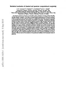
method, the Green's functions for the Barrier region are calculated as above, however the effects of the Leads on the device region of interest are included via a simple self-energy term(s). To see why this can be done, we will consider the discrete (tight binding) model proposed by Datta as shown in Fig. 4. Note that the lattice is discretized as {x,y }=={ia,ja} in the barrier, and {x,y }=={Pia,P ja} in lead L.
lja $a
Figure 4: Schematic representation of the discrete coupli:µg
31
The retarded Green's function for the discretized coupled device (L-B side) is in matrix form -1
(nw - i17)I - HL
T
(69) ,+ where ,(pi, i) == t ==
(nw - i17)I - HB
!:2 is the tight binding equivalent (a is the lattice spacing)
2
of the overlap integral term between orbitals on neighboring sites of the lattice ·and here describes the hopping between neighboring sites of the interface of the barrier ·and the left lead. We solve for the 'barrier region G 13 and obtain
(70) where gi is the uncoupled left lead's retarded Green's function and can be obtained analytically. The 2-D self-energy in the barrier region due to the left lead is ~L(i,j)==[,+gi,Lj==t 2 gi(Pi,Pj)- A similar contribution arises from coupling to the right lead such that the total retarded self-energy due to the coupling to the leads is
~r
==
~L + Ek.
The calculation of the steady state observables of the system such as charge density or current density proceeds as before, with the non-equilibrium Green's function calculated as G+ == G 13 E+GB. The Keldysh type self-energy here is
E+ == E! +~~,and E!,R == -2fL,R(w)Im[EtR(i,j)]. If we go to the ~ontinuum limit by allowing the lattice constant to approach
32
a -+ 0, we find in the 1-D case:
I;~
la-+o= I;Hx, xt, w)
~ -i.S(x -
xt).S(x - L
/,,22mkL.
(71)
Formally Feuchtwang's method can also be viewed as having produced a self-energy, though it is an unpleasant differential operator as in Eq. (67). We seek therefore a method intermediate between the two methods presented. We wish to work in the continuum positio!1 representation, and apply the rigorous Green's theorem method of Feuchtwang to coupling Green's functions obtained. However we wish to treat the coupling to the Leads from the point of view of the inclusion of the self-energy into the Barrier region Green's function as in the self-energy tight binding approach. We have been able to synthesize the results of the two approaches, and that is the subject to which we now turn.
33
CHAPTER SIX: BOUNDARY MATCHING VIA A SELF-ENERGY: CONTINUUM MODEL.
The goal here is to utilize the Green's theorem method for the determination of the Green's function for the entire device, then to concentrate on the barrier region exclusively. The coupling to the Leads will be obtained as a self-energy as in the· Datta (tight-binding) approach. The starting point is again the Green's theorem method. After applying Green's theorem to the various Green's functions as in Eq. (61), we obtained the following Green's functions (in 1-D; the multidimensional case can be treated similarly). This turns out to be simplest if we choose Dirichlet boundary conditions for the leads (gi~ Iboundaries= 0) and '
. .
.
09
r,a
Von Neumann boundary cond1t10ns for the barrier ( ~
.
!boundaries=
0). We
thus obtain for this case of mixed boundary conditions (suppressing w and the retarded/advanced (r, a) superscripts)
G(x, xt)
.
= 9L(x, xt)0(-(x' -
L))
{ri2 - a 9L(x, x1)G(x1, xt) }
+ -2
m 8 X1
,
x R (76) X1=R+
9B(x, xi)0(x - L)0(-(x - R))
(77)
Now we can solve for the barrier region {x, xi E B} by substituting for 8~ 1
G(x1, xi, w) in Eq. (74) from Eq. (77), yielding for example x i > L. (78) The continuity of G and
8
~
1
G across the boundary L allows us to subst itute
the L- side Green's functions for the L + we need in Eq. (78). We thus have
n2 a2 gL( x 1 , x2, ltJ) 2m
ax1ax2
35
G(L+, xi, w), xi> L . (79)
The Right boundary Green's functions are obtained similarly by exploiting the continuity of G and
8~ 1
G across the boundary. Substituting these results
into EQ. (74_) yields the Green's function in the barrier region with the effect of . the leads included:
Qr,a(x, XI, W) == g~a(x,
XI, W )+
(80)
This can be written in Dyson form
Qr,a(x,
JJ
XI,
w) == g~a(x, XI, w)+
git(x, X1, w)~r,a(x1,
X2, W )Qr,a(x2,
(81)
XI, w)dx1dX2,
The continuum representation retarded (advanced) self-energy due to the coupling to the leads can now be seen to be
Comparing this expression with the expression obtained from the tight binding (matrix) Datta approach shows that we have recovered a central result of the tight binding method. This is due to the specific form of the un~oupled Green's functions. Th~ contribution from the uncoupled Green's functions for
36
1-D example) is
kxL,R
=
~/~(hw -
VL,R
± iTJ).
The approach described here is
equally simple for higher dimensions, and is a rigorous and relatively straight . forward approach for modeling mesoscopic heterostructures.
37
CHAPTER SEVEN: APPLICATIONS OF THE METHOD
The Mesoscopic Conductor
Consider the heterojunction depicted schematically in Fig. 5. This is a prototypical 2-D mesoscopic conductor, where the semi infinite leads are metallic electron 'reservoirs' and are considered to be in thermodynamic equilibrium. The middle region is a mesoscopic conductor. The cross section is uniform, and there is no potential in the fj direction. We apply a constant electric field in the
x direction,
region V (X) ==
thereby introducing a linear potential in the middle (conductor)
µ~=zR (R -
X). The applied electric field raises the energy .of the
bottom of the left reservoir's band by eV as well as raising the chemical potential
R
L
Figure 5: Typical 2-D device with uniform cross-section.
38
to µL
+ eV.
We thus have for our left semi infinite lead the following Green's
function equation 2
82 ) ti2 ( a . (nw + 2m a;B2 + 8y2
- eV
+ iry)gI(x, XI, Y, yl, w)
(83)
== &(x - xi)&(y - y1). We can make a simplification by reducing the dimensionality from 2-D to a quasi-1-D case.
We can achieve this by taking advantage of the uniform
fl
direction. That means we can transform the y-dependence into
eigenmodes.
For our device configuration, let us assume that the width is
transverse
small and choose Dirichlet B.C.s for the are easily implemented).
fl direction
(other boundary conditions
Note that the fl-direction eigen-modes are discrete
(small device width). We can expand the Green's function in the fl-direction by a complete orthonormal set of states. The that case is &(y - yl)==i
_I:
fl
coordinate delta function in
sin(~y) sin(~y1), and the Green's function is
m=l
g[(x,xi,y,y',w) ==
i ·I : sin(~y)sin(~y1)g[(x,x1,m,w). Gathering terms, the m=l
PDE equation becomes 2
(nw
2
2
( r,, ~) n, 8 + '-2 - _....;.."---
2m8x
2m
.
r
_
eV + iry)gdx, xi, m, w) - &(x - xi).
(84)
The right region uncoupled Green's function is similarly obtained, but with eV being replaced by zero. The barrier region in this model is a mesoscopic conductor and has the linear
39
potential V(x)=Vs
+
µ~='t (R -
x) due to the external constant electric field
and the bottom of the conduction band energy. The middle region (quasi 1-D) retarded Green's function equation is now
(nw
ri2 a2
+ 2m ax 2
(n m7f )2 -
: 2
- V(x)
+ iry)g~(x, xi, m, w) = c5(x -
xi),
(85)
which has solutions in terms of Airy functions. We obtain for the Barrier region uncoupled retarded Green's function:
(86) where the Wronskian Wr [Ai(-z'); Bi(-z')] is a constant
= -(1/n-).
The short
hand notation of z< and z> mean the lesser and the greater of the two arguments and
z = -a- 2 13 (ax
+ b)
2m l::,,.µ n2 R _ L , b = k~ - aR,
, a=
n2k2m
(nm7r)2
2m
2m
w
=
hw
(87)
+ iry.
If the boundary conditions imposed are Von Neumann (;xg lx=L,R= 0), the factors C L,R are (primes indicate differentiation)
Ai'(-zL,R) CL,R=-B.'( ). 'l -ZL,R
(88)
Thus no new difficulties arise when we attempt to write down the uncoupled barrier region Green's function for the .2-D multi moded case under a ~onstant driving electric field.
40
The coupled retarded Green's function now includes the self-energy contributions from the left and right semi infinite Leads
(nw
+
n2 a2
+
2
m ax 2
(n m1r )2 : 2
-
- V(x)
+ iTJ)G;(x, xi, m, w)
(89)
j Lt(x,x1,m,w)G'ii(x 1,xt,m,w)dx1 =6(x-xt).
The non equilibrium Green's functio_n for the mesoscopic conductor is obtained from the steady state expression R R
a+(x, xt, m, w) =
JJ
Gr(x, X1, m, w)I:+·(x1, X2, m, w)Ga(x2, xt, m, w)dx1dx2,
L
L
(90) and the Keldysh self-energy is
(91) with Ez:, (x 1 , x 2 , m, w)
== -i8(x 1 -x 2 )8(x 1 -L) Nn,kxL
quasi 1-D retarded case is kxL
=
v~(nw - ("!)
, and the momentum for our
2 -
eVL
+ iTJ) with I:'i, obtained
similarly. _Note that
Etiddle
==
0 since the coupling to the leads destroys the (initial) un-
coupled equilibrium state. The presence of phase breaking interactions however, which we are neglecting, such as electron-electron or electron-phonon interactions will give nontrivial results since
Etiddle
-/= 0.
The probability density distribution in the conductor can now be calculated
41
0.?r-----,..---.-------....---~ 0.65 0.6 0.55 0.5 0.45
'"=o---=o:-'".-=2--:o. . . . -4--o. . . . -6--o. . . . -a----......J1 X
Figure 6: Probability density distribution n(x,m) for mode m=l.
VL · 0.3 Ryd and VR
=
0, D
=
VB _ O,
l a.u.
from
(n(x, m))
=
-if [G+(x, xr, m, w)L=x' dw,
(92)
This is shown for m=l in Fig. 6. The current can be calculated from the expression for the non-equilibrium Green's function. In this 2-D case, passing to the continuum limit and setting
x
=L
at one of the internal boundaries for definiteness:
=
-en
2m (21r)
2
/J[(aa + X
8 ,)a+(x,xi,ky,w)] dkydw. 8X x=x'=L
(93)
We then can ·c alculate the (I-V) Current-Voltage dependence for the ·mesoscopic conductor. The I-V profile is shown in Fig. 7.
42
Current Vs. Voltage
0.06 H
0.04
0.02 0 ~:-'""":"~-"-::"°"--::---'"----:::----"~~~~....._____~~___._j
0.1 0.2 0.3 0.4 0.5 0.6 0.7 0.8 V
Figure 7: I-V characteristics of the 2-D mesoscopic conductor. VB Ryd and VR
== 0,
D
==
== 0,
VL
==
0.3
l a.u.
Integer Quantum Hall Effect
At high magnetic fields, the Hall resistance has been experimentally determined to be quantized in units of ( 2~ 2 ) , as was discussed in part one of this thesis. What makes this so unique is that the resistance at high B fields is quantized with an accuracy on the order of a few parts per million. One explanation of this is due to the magnetic field localizing the right-moving electrons and left-moving electrons on opposite sides of the sample. This reduces the overlap between the right and left moving states, and backscattering becomes suppressed even in the presence of impurities[2, 5]. Because of this high accuracy of quantization, the IQHE is used to maintain the resistance standard. In an ordinary classical Hall experiment the Lorentz force causes a transverse
43
charge separation of the right and left moving electrons, leading to a transverse Hall electric field and Hall voltage. Here we consider instead an ideal mesoscopic system with a very high driving voltage. In this case the Hall field will remain .smaller than the longitudinal field. As a first approximation then we will neglect 'it. Consequently we model the mesoscopic quantum Hall conducting bar using the 2-D formalism developed above, with a constant magnetic field in the
z direc-
tion in the middle mesoscopic conductor region. We choose the vector potential such that
A== -y
Bx, and therefore Ax == 0 and Ay == -Bx. The Green's func-
tion for the uncoupled mesoscopic conductor region (with V(x) due to the constant electric field
(nw-
( -ili_Q_
+ eBx ) 2
{)y
2m*
E == -Eox)
µ1.='t (R -
is:
f,,2 8 2 + - a 2 -V(x)+irJ)gB(x,x1,y,y1,w) 2m*
==
x)
x
(94)
o(x - xi)o(y - y1).
For a system of constant width W we can expand gB (x, xi, Y, y1, w) then ( nw -
2 (n (m1r) + eBx ) 2 n 82 ·w +-- V(x) + irJ)g13 (x, xi, m, w) 2
2m*
2m* 8x
== o(x - xi).
44
.
(95)
It is convenient to seek the eigenstates
ri2 a2 (- 2m* 8x2 w h ere
b ==
We
B eI d x ==· --'1i(m1r) == -Im• --'eB -W '-----'-' an m
n(~)eB m• -
b2 2a
i
+ 2m*w~(x + Xm)2 -
flµ
D' and C ==
flµm • D(eB) 2
--l...--
1i2(~)2
fl R
re-define th~ energy as
E ==
a2 ( - -2 8q
liliw
We
+
-
lie
2
We
and qm
= [~Xm],
and
to obtain
+ (q + qm) )cp(q) '
One last transformation of the form
1 * 2 2 m w c,
We proceed analogously-to Datta[2]
2
b1i We
2a
(96)
Th e constants are a -
•
= [~x]
and transform the coordinates as q
== 1iwcp(x),
.
+ T-
2 m•
+ C)cp(x)
== 2Ecp(q).
c; == q + qm
(97)
leaves us with a more compact
form
a2 2 (- ae + t )cp(f) == 2Ecp(f).
(98)
The general solution of Eq. (98) is comprised of Hermite polynomials and Hypergeometric (Kummer) functions such that (rewrite in terms of q + qm) 2
cp(q) = e- µL ,
J-1,R)- Note that here µL===µR+eV, where eV. === ~µ===bias.
presupposes a chemical potential associated with a global particle reservoir. Note that a global particle reservoir picture can be recovered in our present case if we define µL === µR and let the applied field (~µ) be the source of nonequilibrium.
Spin-Dependent Transport The extension to include spin dependent transport is straightforward. The left and right leads (see Fig. 8) are now taken to be ferromagnetic metals held a t thermodynamic equilibrium. At the level of the microscopic theory we are d iscussing, the spin can be included as yet another index (degree of freedom) in our Green's functions, and a spin-spin interaction potential included in the Hamil. tonian for the ferromagnetic regions. This is represe~ted schematically i~ Fig. 9.
49
FM
.!, ~µ ------------
t
R
L
t
0
Figure 9: Potential energy profile for the spin-dependent case. The semi-infinite left and right leads are ferromagnetic metals in thermodynamic equilibrium. The middle region is an insulating barrier.
The magnetoresistance of a ferromagnetic metal-insulator-ferromagnetic metal, or FM-I-FM junction can be written as[3] (109)
where the arrows denote the magnetization direction of the separate left and right ferromagnetic sections (reservoirs), here assumed to be identical types of ferromagnets. In terms of the Green's function·s, the ferromagnetic sections of the device will be described by the usual free particle Hamiltonian, plus a spin-spin interaction potential ~ We can write the spin dependent single particle (the i
50
th
particle)
Hamiltonian for the left ferromagnetic region as
(110) where -J is the ferromagnetic(J
> 0) constant coupling strength in this picture.
The only restrictions to be imposed are the self consistency requirements of fixing the particle number thro~gh the chemical potential. The magnetization per particle is related to the average of the spins
M
== (S)
N,.
(111)
We can introduce a mean field like simplification if we average over one of the spin variables so that the spin-spin interaction potential becomes ½ = "'
N
"'
-JSi · I:(Sj)
==
"'
-JSziNM (choosing the magnetization to be in the zdirection).
j
The Hamiltonian then takes the simpler i th particle form (112) Also, let us assume that the spin operator in Eq. (112) operates on an eigenfunction as SiXaJf)=cri Xai (f) ([14]) where here the spin eigenvalues are the (unit) electronic spin eigenvalues of {cri E+l,-1}. Any constants such as
n can
be absorbed into -J and that in turn rendered dimensionless. The spin eigenfunctions form the usual type of a complete orthonormal set of states such that the .orthonormality condition yields the following spin . Kronecker delta function
J Xa-i (f) Xa-j (f )df =
b"a-wj. We rewrite the Left region ferromagnetic reservoir
51
Green's function equation under a constant electric field in the i; direction (which shifts the bottom of the Left region band energy by e V == bias Right region, eV
==
== 13..µ.
In the
0) as
(nw ·+
ri2 2
m
=t
v; + JaiNM -
eV + i'TJ)gL,./x, xi, y, y1, w)
(113)
== J(x - xi)J(y - y1). Here we will consider a 3-D system large and uniform in the transverse directions. [See Fig. (8).] That means we can choose periodic B.C. and Fourier transform the {y, z} dependence into {ky, kz} dependence. Other conditions can be easily implemented. For the sake of brevity ( and clarity), we will suppress the z dependence as. it can be handled analogously to the y dependence. The y-coordinate delta function in this case is b(y - y1)
==
Ym.ax
J
e+iky(y-y') ~,: and the
Ym.in
Green's function equation becomes (similarly for the Right region with eV-+ 0)
ri2 a2
(nw+ max 2 2
:n
(nk ) 2 -
2
+JaNM-eV+i'TJ)gt,(x,xl,ky,w)
(114)
·== J(x - xi). The barrier region in this model is an insulator and again has the linear potential V(x)
==
µ~='iR (R -
x) due to the external constant electric field. The
barrier (quasi 1-D) retarded Green's function equation is now
(hw
ri2 a2 +2 2m8x
(nk ) 2 Y
-
2m
V(x)
== J(x - xi).
52
+ i'TJ)gfu(x, xi, ky,w)
(115)
As discussed in the first part of the thesis, the non-equilibrium Green's function for the device is needed in order to calculate any observables (such as the current) of interest. In this case we will calculate the spin dependent current . density, and by integrating over ky, we will calculate the current for Itt and JH and therefore R
ti
== (µL-µR)/e and ltt
R
-
H -
(µL-µR)/e lt.1-
The current density is calculated from the non equilibrium Green's function for the entire device which was obtained from the uncoupled retarded and advanced Green's functions which are sol11;tions of equations (114,115). These uncoupled Green's functions are solved similarly to the prototypical case of the mesoscopic conductor discussed in · a previous chapter. The expression for the spin dependent current density is (restoring the z-dependence)
(It.I- (x)) ==
-en
2m (21r)
3
/
/
[(·aa + aa,) c+(x, xi, ky, kz, w)] X
X
.
dk~dw.
(116)
x=x'
Numerical calculations of the spin dependent current and magnetoresistance were carried out. The results are shown in Fig. 10. We note in Fig. 10 a negative magnetoresistive behavior. This agrees with an earlier calculation by Wang [4] who used a different treatment of the leads and the coupling. We can see that this negative differential resistance behavior of the magnetoresistance might have possible device applications in the high bias regime. Previously, investigations into device applications have considered the low bias regime. If we investigate the origin of the magnetoresistance becoming negative at
53
(1) -~
~
co
~ 0. ·r-1
~ 0. H 0 .µ
0•
cu
~ s
0.4 0.6 0.8 Bias ·
co
1
Figure 10: Magnetoresistance vs. bias curve.
high bias, we are led to examining the up-up and the up-do_w n current densities and therefore the R tt =
µL-µR
ltt
and R ti =
µL-µR
lti
spin dependent resistances
that contribute to the magnetoresistance. There we find .that the magnitude of the up-down current density becomes larger than the up-up current density at a high enough bias. This is due to the bias becoming much larger than the ferromagnetic energy splitting. The values of the bias coincide with the value of the bias at which the magnetoresistance becomes negative as can· be seen in Fig. 11. Note that we are not limited to the FM-I-FM configuration. We can model the I-V characteristics of the spin injection into a metallic conductor (FIV1-MFM) as this is a reasonable device configuration. This we do by simply tuning the bottom of the conduction band energy in the central region to VB
54
= 0.
In
~
·r-1 CJ)
i:::
a, "O
0. 04 0.03
.w 0.02 i::: H H ::1 Q)
u
0.01
o.____..___.......______.,__ 0.2
0.4
0.6
0.8
___._j
1
Bias
Figure 11: Aligned and Anti-aligned current vs. bias
the case of an insulating barrier, appreciable currents were found only for very short barrier lengths. In the conducting case, interesting behavior is found as the device length changes. Figs. 9-14 show I-V characteristics and the magnetoresistance for barriers of length 1,6,and 10 atomic units (a.u.). The complicated structures are a consequence of resonances.
55
0.02 0.0175 ~
0.015
Q)
t
0.0125
~
u
0.01 0.0075 0.005 0.1
0.2
0.3
0.4
0.5
0.6
0.7
0.8
bias
Figure 12: Current vs. bias. Anti-aligned case (tt). Length=l a.u .
0.02
..................-....----=:::.=--:::..'"::-....,......-..........-...--~~
0 . 018 .µ
0.016
@ 0.014 J..t J..t 5 0.012 0.01 0.008 0.1
0.2
0.3
0.4
0.5
0.6
0.7
0.8
bias
Figure 13: Current vs. bias. Aligned case (tt). Length=l a.u.
56
0.4 0.3 0.2 0.1 0
0.1
0.2
0.3
0.4
0.5
0.6
0.7
0.8
Figure 14: Magnetoresistance vs. bias. Length==l a. u.
0.02 0.0175 .jJ
@ 0.015 ~ u
0.0125 0.01 0.0075
_
_ 0.6
0.005 ...__.....__...._ _.___.______. 0.1 0.2 0.3 0.4 0.5 bias
__._~
_ 0.8 __._,
0.7
Figure 15: Current vs. bias. Anti-aligned. Length==6 a. u.
57
o.0225r.....--~..,.......~~:::::====:::::::=:===-7 0.02 0.017 _5
.u
@ 1-1
0.015
~u 0.0125 0.01
0.1
0.2
0.3
0.4 0.5 bias
0.6
0.7
0.8
Figure 16: Current vs. bias. · Aligned. Length==6 a.u.
0.2 0.15 0.1 0.05 0 0 .1
0 . _2
0 .3
0.4
0 .5
0.6
0.7
0.8
Figure 17: Magnetoresistance vs. bias. Length==6 a. u.
58
0.0175
~
QJ
0.015
~ 0.0125
;:j
tJ
0.01 0.0075 0.005 0.1
0.2
0.3
0.4 0.5 bias
0.6
0.7
0.8
Figure 18: Current vs. bias. Anti,- aligned. Length==lO a.u.
0.02 0.0175 ~
@ 0.015 1-1
~ 0.0125
tJ
0.01 0.0075
1=-~o~.a
0 ·• 0 os 1....:--_-1_0......-2_o......3--0~-4-0:--'.-:'.:5---::o:-"'.~6~0....... 0
bias
Figure 19: Current vs. bias. Aligned. Length=lO a.u.
59
0.15
0.1
0 . 05
0
0.1
0.2
0.3
0.4
0.5
0.6
0.7
0.8
Figure 20: Magnetoresistance vs. bias. Length=l0 a .u.
60
CHAPTER EIGHT: APPLICATION OF GENERALIZED NON-EXTENSIVE STATISTICS TO COMPLEX RANDOM SYSTEMS
Introduction
Financial markets are complex random systems. Markets are comprised of many interacting investors each with their own trading strategy and their own outlook on the particular market. The task of tracking individual investors' behavior, and their subjective interpretation of events (and hence their reactions to events) is a daunting, if not outright impossible task. In fact, it is akin in complexity to a many body problem in physics. This has been realized over time, and hence a statistical approach of price changes rooted in the random walk was rightfully adopted as early as the turn of the 20th century, beginning with the work of L. Bachelier[22]. This sort of statistical approach to market dynamics has in the past few decades yielded deeper understanding of .the dynamics and stochastics (randomness) inherent in markets. These efforts have yielded such seminal works as the Black-Scholes derivatives pricing model and generalized stochastic models
61
for the price changes, and the modeling of the interacting investor behavior directly via lattice-like models. When it comes to application to real markets, there are inconsistencies between the models and the real data. In short, the distribution of price changes in a real market has 'heavy' (power law) tail_s;-that is, there is a greater chance of outlyers to occur than in a gaussian distribution. Also, the noisy dynamics are not simulated well by the normal (Gaussian) distributed noise. The random walk described by real random complex systems is one of super-diffusive or sub-diffusive behavior more often than not. This stems from the fact that these systems are in reality open systems, and also from the correlation (statistical dependence) of subsequent realizations. The case of super- and sub-diffusion have been approached in many ways. A recent approach has been the Tsallis[24] generalized non-extensive statistics. These statistics allows for a natural description of super- and sub-diffusive behavior as well as the power law 'heavy' tails of the distribution. In the following, a non-extensive model for stock markets is given, as well as the derivatives and options that would then be written on such a primary market. We thus obtain a new statistical description of the statistics of price changes, and generalize the Black-Scholes derivatives pricing model.
62
Financial Market Dynamics
Several financial markets' indices and their member stocks are characterized by price changes whose variances have _been shown to undergo anomalous (super) diffusion under time evolution. [20, 21, 22] This means that the variance scales with time as a power law, a 2(t) and H
=/-
rv
tH where the case H
== l is the normal process
l corresponds to anomalous diffusion. Moreover, the probability distri-
butions of the price changes have power law tails [28, 21, 22]. An open long-term question is how best to describe these distributions and the corresponding time evolution of the moments. In this approach we show that a possible description can be found using the maximum entropy method[23], with a non-extensive Tsallis entropy that allows a generalization of the statistics so that we can describe the anomalous diffusion process exhibited by the markets[24, 25, 26]. This is illustrated for the S&P500 index, but may be applicable to model the superdiffusion and power law behaviors observed in a broad range of markets and exchanges [22, 40, 31]. The description we will use was developed in the general context of anomalously diffusing systems by Tsallis and Bukman[24] and Zanette and Alemany[25] . Here we briefly summarize their derivation, whic~ is based on a maximization of entropy subject to certain constraints. The point of departure from normal maximum entropy approaches is the feature that the entropy used is the non-
63
extensive Tsallis entropy, (117) Here P(x, t) is the Tsallis probability distribution and is a function of say, price changes x(t) == price(r
+ t)
- price(r). The time intervals are t == tlr, the
trading time intervals (here, in minutes) in which we measure the price changes. The Tsallis parameter q characterizes the non-extensivity of the entropy. (It is restricted to 1 < q < 3 for super-diffusion). In the limit q -+ l the entropy becomes the usual logarithmic expression 8==- JP ln P. Associated with the non-extensive entropy is the use of the constraints
(x - x(t)) 9
=
((x - x(t))2) 9
-
j P(x, t) dx = I, j [x - X(t)]P(x, t) dx = 0, j [x - X(t)] P(x, t)9 dx = 9
2
o-9 (t)2.
(118) (119) (120)
The first of these is simply the normalization of the probability. However, in the latter two equations the probability distribution function is raised to the power q. Unless q == l these are not the usual constraints leading to the mean and
variance, and aq (the 'q-variance') is not the ordinary variance. Maximizing the Tsallis entropy subject to these constraints, Tsallis and Bukman obtained [24]
P(x, t)
=
1
Z(t)
{1 + fJ(t)(q -
64
-
_l_
I)[x - x(t)]2} •-• ,
(121)
The partition function and q-variance are given by
B(l Z(t)
_1) 2
(122)
Jf3(t)(q - 1) ' 1
a~(t) Here B(x, y)
_1
2' q-1
(123)
2f3(t)Z(t)q-l.
= I'(x)I'(y)/I'(x + y) is Euler's Beta function. An important prop-
erty of the probability distribution function Eq. (121) pointed out by Tsallis et al. and Zanette et al. is that, with appropriate time-dependent parameters, it
is the solution of a time evolution equatio:r:i which leads naturally to anomalous diffusion[24, 25]. Consider the nonlinear Fokker-Planck equation
aP(x, t)µ = _!_ [F . ( )P(
at
ax
X
where F(x) is a linear drift force, F(x)
)µ] X'
t
D a P(x, t)v 2
+
2
ax 2
'
(124)
== a-bx. One can show that a probability
distribution function of the form Eq. (121) solves this [24], as long as (125)
q==l+µ-v
and the time dependences of the parameters are given by
dzµ+v(t) µ + ll dt µ
+ 2vDf3(0)Z(0) 2µ - bzµ+v == 0,
-dx == a - bx.
(126) (127)
dt
Normalization is preserved only for the case µ
==
l, and we specialize to that
case. We also identify a time independent quantity Nq, the product of the inverse
65
variance and the partition function (squared) of the process at any time,
2 2 2 B (½,q~1-½) (3(t)Z(t) == (3(0)Z(O) == Nq == - - - -
(128)
(q - 1)
The inverse of the regular variance (henceforth the 'inverse variance' (3(t) in Eq. 128) then evolves as
(3(t) == [
(fJ(t )'1--?- 0
2
4(2 - q)DNqy) e-b(3-q)(t-to) 2b
+ 4(2 -
q)Nqy]
q-3
2b
(129) One can perform numerical simulations of Tsallis distributed random processes and their moments in many ways including the use of the underlying Stochastic Differential Equations [30, 32]. We numerically simulate Tsallis distributed random numbers and their moments and compare the results as follows. We choose values for the diffusion constant D, the non-extensivity parameter q, the force constant b(a
==
0), and the initial (3(t 0 ) . Note that a knowledge of q
immediately gives Nq by Eq. (128) and so we also have the initial Z(to) and thus
Z(t) and (3(t). We evolve the inverse variance (3(t) according to Eq. (129) and calculate the mean from Eq. (126). We generate Tsallis distributed random numbers (at each time t) that have the time evolved values of (3(t) and q from a uniformly distributed set of random numbers. We can relate these two random processes by a transformation such as the one discussed in Numerical Recipes[35]. That is, for a uniform distribution,
66
we have
dy,
O