tions given by the Author and lodged in the John Rylands University Library of. Manchester. Details may be .... implementation is studied with the aim of determining the chief algorithmic and ...... of all virtual memory locations for which it holds valid data. ...... UFO - United Functions and Objects Draft Language De- scription ...
TECHNIQUES FOR IMPROVING THE PERFORMANCE OF PARALLEL COMPUTATIONS A thesis submitted to the University of Manchester for the degree of Master of Science in the Faculty of Science and Engineering
October 1996
By Graham D. Riley Department of Computer Science
Contents Abstract
7
Declaration
8
Copyright
9
Education and Research
10
Declaration
10
Acknowledgements
11
1 Introduction
12
1.1 1.2 1.3 1.4
Overview . . . . . . . . . . . . . . . . The \Best" Implementation Problem An Outline of the Method . . . . . . Outline of the Thesis . . . . . . . . .
. . . .
. . . .
. . . .
. . . .
. . . .
. . . .
. . . .
. . . .
. . . .
. . . .
. . . .
. . . .
. . . .
. . . .
. . . .
. . . .
2 Background
12 13 16 18
20
2.1 Parallel Execution . . . . . . . . . . . . . . . . 2.1.1 Matrix Addition . . . . . . . . . . . . . 2.1.2 Triangular Matrix-Vector Multiplication 2.1.3 Parallel Classi cation . . . . . . . . . . . 2
. . . .
. . . .
. . . .
. . . .
. . . .
. . . .
. . . .
. . . .
. . . .
. . . .
21 22 24 26
2.2
2.3 2.4 2.5 2.6
2.1.4 Summary of Examples . . . . . . . . . . . . . . . Machine Models . . . . . . . . . . . . . . . . . . . . . . . 2.2.1 RISC Processors and Hierarchical Memory Access 2.2.2 Multicomputers versus Multiprocessors . . . . . . 2.2.3 Summary of Machine Models . . . . . . . . . . . Programming Models . . . . . . . . . . . . . . . . . . . . Memory Consistency Models . . . . . . . . . . . . . . . . Related Work . . . . . . . . . . . . . . . . . . . . . . . . Summary . . . . . . . . . . . . . . . . . . . . . . . . . .
. . . . . . . . .
. . . . . . . . .
. . . . . . . . .
. . . . . . . . .
. . . . . . . . .
3 Performance Analysis and Modelling 3.1 Performance Modelling . . . . . . . . . . . . . 3.2 Review of Performance Modelling . . . . . . . 3.2.1 PRAM Models . . . . . . . . . . . . . 3.2.2 LogP . . . . . . . . . . . . . . . . . . . 3.2.3 BSP . . . . . . . . . . . . . . . . . . . 3.2.4 Hockney's Performance Parameters . . 3.2.5 Foster's Multicomputer . . . . . . . . . 3.3 Mixing Analysis with Experiment . . . . . . . 3.4 A Description Method for Program Behaviour 3.4.1 Amdahl's Law . . . . . . . . . . . . . . 3.4.2 Amdahl's Law|Example . . . . . . . . 3.4.3 A More Realistic Analytical Model . . 3.4.4 Load Imbalance . . . . . . . . . . . . . 3.5 Summary . . . . . . . . . . . . . . . . . . . .
4 An Overview of the KSR1
31 32 33 34 36 37 39 42 42
44 . . . . . . . . . . . . . .
. . . . . . . . . . . . . .
. . . . . . . . . . . . . .
. . . . . . . . . . . . . .
. . . . . . . . . . . . . .
. . . . . . . . . . . . . .
. . . . . . . . . . . . . .
. . . . . . . . . . . . . .
. . . . . . . . . . . . . .
. . . . . . . . . . . . . .
. . . . . . . . . . . . . .
44 46 46 47 49 51 53 54 57 58 58 59 60 62
64
4.1 The KSR1 Architecture . . . . . . . . . . . . . . . . . . . . . . . 64 3
4.2 The KSR1 Programming Model . . . . . . . . . . . . . . . . 4.2.1 The KSR1 Tile Statement . . . . . . . . . . . . . . . 4.3 Costs Associated with the KSR1 . . . . . . . . . . . . . . . . 4.3.1 KSR Directives . . . . . . . . . . . . . . . . . . . . . 4.3.2 KSR1 Memory Latencies . . . . . . . . . . . . . . . . 4.3.3 Synchronisation Primitives|Locks and Barriers . . . 4.3.4 Memory System Behaviour|Alignment and Padding 4.4 Executing on the KSR1 . . . . . . . . . . . . . . . . . . . . . 4.5 Performance Monitoring Support Tools . . . . . . . . . . . . 4.5.1 Accurate Timers . . . . . . . . . . . . . . . . . . . . 4.5.2 The Performance Monitor PMON . . . . . . . . . . . 4.5.3 GIST|a Graphical Event Monitor . . . . . . . . . . 4.5.4 PRESTO Facilities . . . . . . . . . . . . . . . . . . . 4.6 Illustrative Experiments on the KSR1 . . . . . . . . . . . . . 4.6.1 Load Imbalance . . . . . . . . . . . . . . . . . . . . . 4.7 Summary: Framework for the KSR1 . . . . . . . . . . . . .
. . . . . . . . . . . . . . . .
. . . . . . . . . . . . . . . .
. . . . . . . . . . . . . . . .
5 An Example Application
66 67 68 68 69 69 70 71 72 72 73 74 74 75 75 78
80
5.1 The N-body Application . . . . . . . . . . . . . . . 5.2 The Initial Implementation . . . . . . . . . . . . . . 5.2.1 Initial Implementation of the N-body Code . 5.2.2 Application Parameters . . . . . . . . . . . 5.2.3 Parallel Algorithm Development . . . . . . . 5.3 Summary . . . . . . . . . . . . . . . . . . . . . . .
6 Analyses Of An Application
. . . . . .
. . . . . .
. . . . . .
. . . . . .
. . . . . .
. . . . . .
. . . . . .
. . . . . .
80 81 82 86 86 88
89
6.1 Serial Results: Version 0 . . . . . . . . . . . . . . . . . . . . . . . 89 6.2 Version 1: Locking Strategies . . . . . . . . . . . . . . . . . . . . 91 4
6.3
6.4
6.5
6.6
6.2.1 Introduction to the Analysis . . . . . . 6.2.2 Analysis of Lock Costs . . . . . . . . . 6.2.3 Overhead Anomaly . . . . . . . . . . . 6.2.4 Version 1 Conclusion . . . . . . . . . . Version 2: Local Accumulation . . . . . . . . 6.3.1 Analysis External to FORCES . . . . . 6.3.2 Internal Analysis of FORCES . . . . . 6.3.3 Summary of Version 2 . . . . . . . . . Version 3: Sequential Spatial-Cell Techniques 6.4.1 Implementation Description . . . . . . 6.4.2 Sequential Results Discussion . . . . . 6.4.3 Summary of Version 3 . . . . . . . . . Version 4: Parallel Spatial-cells . . . . . . . . 6.5.1 Parallel Implementations . . . . . . . . 6.5.2 Overhead Analysis . . . . . . . . . . . 6.5.3 Summary of Version 4 . . . . . . . . . Conclusion . . . . . . . . . . . . . . . . . . . .
. . . . . . . . . . . . . . . . .
. . . . . . . . . . . . . . . . .
. . . . . . . . . . . . . . . . .
. . . . . . . . . . . . . . . . .
. . . . . . . . . . . . . . . . .
. . . . . . . . . . . . . . . . .
. . . . . . . . . . . . . . . . .
. . . . . . . . . . . . . . . . .
. . . . . . . . . . . . . . . . .
. . . . . . . . . . . . . . . . .
. . . . . . . . . . . . . . . . .
7 Conclusions
92 96 99 101 101 102 107 114 115 116 118 123 124 124 127 129 130
131
7.1 Summary . . . . . . . . . . . . . . . . . 7.2 Critique . . . . . . . . . . . . . . . . . . 7.3 Further Work . . . . . . . . . . . . . . . 7.3.1 Widening the Experience Base . . 7.3.2 Supporting the Expert Developer 7.3.3 Automation and Intelligence . . .
A Source Code
. . . . . .
. . . . . .
. . . . . .
. . . . . .
. . . . . .
. . . . . .
. . . . . .
. . . . . .
. . . . . .
. . . . . .
. . . . . .
. . . . . .
. . . . . .
. . . . . .
131 133 134 134 135 135
137
A.1 Version 0: Original Sequential Code . . . . . . . . . . . . . . . . . 137 5
A.2 A.3 A.4
A.5
A.1.1 MAIN Program . . . . . . . . . . . . . . . A.1.2 Subroutine FORCES . . . . . . . . . . . . Version 1: Locking Strategies, Parallel . . . . . . A.2.1 Subroutine FORCES . . . . . . . . . . . . Version 2: Local Copies, Parallel . . . . . . . . . . A.3.1 Subroutine FORCES . . . . . . . . . . . . Version 3: Spatial-cells, Sequential . . . . . . . . . A.4.1 Subroutine FORCES, tile Implementation A.4.2 Subroutine FORCES, cell Implementation A.4.3 File data.inc . . . . . . . . . . . . . . . . . A.4.4 Subroutine MAKELIST . . . . . . . . . . A.4.5 Subroutine REORDER . . . . . . . . . . . Version 4: Spatial-cells, Parallel . . . . . . . . . . A.5.1 Subroutine FORCES, tile Implementation A.5.2 Subroutine FORCES, cell Implementation
. . . . . . . . . . . . . . .
. . . . . . . . . . . . . . .
. . . . . . . . . . . . . . .
. . . . . . . . . . . . . . .
. . . . . . . . . . . . . . .
. . . . . . . . . . . . . . .
. . . . . . . . . . . . . . .
. . . . . . . . . . . . . . .
. . . . . . . . . . . . . . .
B Experimental Data B.1 Version 0 . . . . . . . . . B.2 Version 1 . . . . . . . . . B.2.1 External PMON B.2.2 Internal PMON .
137 140 141 141 142 142 143 143 144 145 145 146 147 147 149
151 . . . .
. . . .
. . . .
. . . .
C Assembler Code
. . . .
. . . .
. . . .
. . . .
. . . .
. . . .
. . . .
. . . .
. . . .
. . . .
. . . .
. . . .
. . . .
. . . .
. . . .
. . . .
. . . .
. . . .
. . . .
152 154 154 156
158
C.1 Version 0 . . . . . . . . . . . . . . . . . . . . . . . . . . . . . . . . 158 C.2 Version1 . . . . . . . . . . . . . . . . . . . . . . . . . . . . . . . . 163 C.3 Version2 . . . . . . . . . . . . . . . . . . . . . . . . . . . . . . . . 167
Bibliography
171 6
Abstract Developing parallel implementations of applications which utilise an acceptably large fraction of the peak performance of current high performance computers has proved a di�cult task. The lack of success in this endeavour is perceived as a major impediment to the general acceptance of high performance computing in industry. Even for structured, `static', scienti c and engineering applications coded in FORTRAN, where performance is apparently predictable, success has been limited. This Thesis argues that, while the development of high performance applications for parallel systems remains an experimental task suitable only for the expert programmer, systematic techniques, which maximise the bene t of programmer e�ort, can be employed in order to develop `good' parallel implementations rapidly. A framework for such a method is presented, and a set of supporting techniques is developed, by means of a series of examples on the Kendall Square Research, KSR1. The method requires the achieved performance of an implementation to be described in terms of an `ideal' parallel performance, plus a small number of (parallel) overhead terms. Once the magnitude of each overhead term has been quanti ed, a systematic, iterative, process of overhead minimisation can take place. The source of each targeted overhead is analysed, and an alternative implementation, which reduces the overhead, is developed. Analysis of the overheads requires a mixture of experiment and modelling. 7
Declaration No portion of the work referred to in this thesis has been submitted in support of an application for another degree or quali cation of this or any other university or other institution of learning.
8
Copyright Copyright in text of this thesis rests with the Author. Copies (by any process) either in full, or of extracts, may be made only in accordance with instructions given by the Author and lodged in the John Rylands University Library of Manchester. Details may be obtained from the Librarian. This page must form part of any such copies made. Further copies (by any process) of copies made in accordance with such instructions may not be made without the permission (in writing) of the Author. The ownership of any intellectual property rights which may be described in this thesis is vested in the University of Manchester, subject to any prior agreement to the contrary, and may not be made available for use by third parties without the written permission of the University, which will prescribe the terms and conditions of any such agreement. Further information on the conditions under which disclosures and exploitation may take place is available from the head of Department of Computer Science.
9
Education and Research
The author graduated from the University of Manchester in 1978 with a BSc(Hons) in Physics. After obtaining a PGCE from Christ College Liverpool, and completing his probationary teaching year, he moved into the area of real-time systems simulation in industry, rst with Redifusion Flight Simulation in Crawley, then with Ferranti Computer Systems in Cheadle, Manchester, before joining the Centre for Novel Computing in the Department of Computer Science at the University of Manchester in 1990.
10
Acknowledgements I would like to thank the following|
CNC people past and present for the stimulating tea breaks, in particular Mark, Rupert, Rob and Andy. Also John, for both the opportunity and his patience; Mum and Dad for all their support and encouragement through the years; and nally Pat, for making it all worthwhile.
11
Chapter 1 Introduction 1.1 Overview Parallel computers have so far failed to ful l their promise of providing cheap high performance computing, in part because of the high cost of software development required to nd a suitable implementation of an application which runs e�ciently on a given parallel system. This latter problem has been termed the \best" implementation problem [CL93]. Software development for parallel systems is made di�cult because of the many run-time factors which a�ect execution time. Execution time is, in general, unpredictable and, often, decisions made early in the development process can have profound e�ects on the ultimately realisable performance of an application. Attempts to automate parallel development through, for example, the use of auto-parallelising compilers, rely on some level of performance prediction, and are thus limited to a relatively small class of `static' applications (typically scienti c and engineering applications which are to be coded in FORTRAN) where execution time is not dominated by run-time e�ects. This Thesis presents a method for describing the behaviour of parallel programs executing on distributed memory architectures. The description method captures the achieved execution time of a program in terms of a modi ed Amdahl's Law, which includes terms for various overheads incurred during parallel 12
1.2. THE \BEST" IMPLEMENTATION PROBLEM
13
execution. It is suggested that this description method leads naturally to a systematic methodology for analysing and improving program performance. The existence of such a methodology allows \good" implementations to be found rapidly, approximating a solution to the \best" implementation problem. The method requires the measurement and analysis of the run-time behaviour of an application. This process is illustrated for execution on a Kendall Square Research KSR1-32, a Virtual Shared Memory Multiprocessor, and techniques for measuring speci c overheads and analysing their source are developed for this machine. Foster [Fos95] gives several reasons why users turn to parallel computing, for example, to reduce run-time, to execute larger problems, or to achieve improved accuracy in solution. The method presented here concentrates on improving a particular execution of a program (data set size, etc.) on a certain con guration of target computer (number of processors, etc.). Finding the best implementation in the large con guration space of varying problem size and varying number of processors is beyond the scope of this Thesis. Changes to execution behaviour as the number of processors applied increases is the natural focus of the method; the implications of changing the data set size are addressed in [Car89, Gus88, CL93] 1. A review of current research into machine and programming models, and performance analysis and modelling approaches is included in order to give insight into the origins of the overheads incurred during execution on a parallel machine.
1.2 The \Best" Implementation Problem In order to use a computer to solve an application problem, the problem must be cast in a computable form. For example, in numerical applications which are 1 Increasing the data set size can be bene cial to parallel performance (`speed-up'), since the
parallel overheads tend to become a smaller fraction of the overall execution time, particularly if the computation grows `quickly' with data-set size; for example, if data set size grows as n2 for data-set size n.
14
CHAPTER 1. INTRODUCTION Application problem
Computable solutions
Implementations
Figure 1.1: The implementation space.
speci ed in terms of partial di�erential equations, with appropriate boundary conditions, a discretisation method for the equations has to be chosen. Several alternatives exist: for example, nite di�erence, nite element, nite volume methods. The choice of discretisation method is strongly related to the application problem, and the chosen method of specifying boundary conditions [Car89]. The discretisation process leads to a computable solution being speci ed for the application. The next step is to encode the chosen computable solution in some programming language. In this step, speci c algorithms and data structures are chosen which de ne and control the computation required to solve the application problem [Gur93]. These choices de ne an implementation of the computable solution. The design choices determine the parallel overhead which will be incurred during execution of an implementation. As the sources of parallel overhead are often inter-dependent, a complex design trade-o� space results. The relationship between an application problem, computable solutions and implementations is shown diagrammatically in Figure 1.1.
1.2. THE \BEST" IMPLEMENTATION PROBLEM
15
The problem of nding the best implementation can be viewed as an optimisation problem which seeks to minimise (parallel) execution time across all possible implementations. The number of possible (parallel) implementations which result from the complex design trade-o� space is large and exhaustive searching is not possible. Research into compilation methods shows that aspects of this problem are in fact NP-complete 2 [Obo92]. In such circumstances, heuristics, based on expert knowledge and experimental data, provide a possible means of nding an approximate solution. The method proposed here can be seen as an attempt to identify useful heuristics and systematic ways to apply them. Future research may identify the extent to which this process can be automated. The task, suggested by Figure 1.1, is to nd a way of navigating this implementation space in such a way as to discover acceptable, \good" implementations quickly. The search process is clear: identify suitable computable solutions, choose candidate implementations for these solutions, implement the candidates, understand their execution behaviour and, on the basis of this, move through the implementation space by selecting new implementations. The criteria for choosing candidate implementations must include some notion of the performance improvement to be gained, and the e�ort (or cost) of implementing the proposed candidates. The search will terminate when: (i) an implementation of acceptable performance is found, (ii) a su�ciently understood implementation is found, which indicates that further work is not cost e�ective, or (iii) e�ort runs out. As in most optimisation techniques, a certain amount of backtracking may be required (up into the computable solution space, if necessary), and it is important to ensure that the search has not become trapped in a local minima which is far from the optimal solution. 2 Determining a partitioning of FORTRAN arrays to minimise remote data accesses, for
example.
16
CHAPTER 1. INTRODUCTION
In practice, a search may start with a sequential implementation of the application, where many design decisions and optimisations have already taken place. Some of these may be detrimental to the search for a good parallel solution|for example, a computable solution may have been chosen which includes the choice of discretisation technique and linear algebra solution method which are both unsuitable for parallelising on the target system. It should be clear that more e�ort will, in general, be required to backtrack up into the computable solution space than to backtrack within the implementation space. Auto-parallelising compilers [Obo92] work below the computable solution level, once the solution has been cast into a programming language.
1.3 An Outline of the Method In this Section, an overview of the use of the proposed development method is given. The implementation space is navigated as successive candidate implementations of computable solutions are selected. The execution behaviour of each implementation is studied with the aim of determining the chief algorithmic and machine-speci c factors that a�ect performance. Execution of the implementation is monitored, and the run-time categorised into an idealised parallel execution time plus a set of parallel overheads. The method is supported by an analysis of the algorithmic requirements for activities, such as computation, remote data access and synchronisation, and by a set of machine-speci c costs which support these activities. This process is known as performance modelling. In `static' applications, performance modelling may explain the observed behaviour completely, as execution time is predictable. When execution time is unpredictable (in `dynamic' applications), modelling can be used to help analyse experimentally observed behaviour.
1.3. AN OUTLINE OF THE METHOD
17
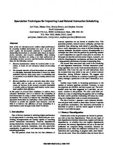
Simulation Performance (time steps/s) 0.20 0.18 0.16 0.14 0.12 1/T
Naive Ideal Realistic Ideal Achieved
0.10 0.08 0.06 0.04 0.02 0.00 0
4
8
12
16
20
Number of processors
Figure 1.2: A typical performance graph produced as a result of the application of the method. The results of analysing candidate implementations are summarised in performance curves, plotting 1=T against p (where T is execution time and p is the number of processors). Examples of the kind of performance curves which may be plotted for a candidate implementation is given in Figure 1.2. These are:
� |a naive ideal curve (actually a line), the rst term of an Amdahl law expansion modelling the performance (p=T ), where T is a reference time, (usually the sequential execution time of the implementation, but the time of the parallel implementation on a single processor may sometimes be used), and p is the number of processors (see below).
� |realistic ideal curves, which include known lower bounds on the overheads inherent in the algorithm/implementation (e.g. unparallelised code).
� |achieved curves, showing the actual performance achieved. The method then requires that any signi cant di�erence between the realistic
CHAPTER 1. INTRODUCTION
18
ideal curve and the achieved curve(s) be accounted for by an overhead analysis. Di�erent ideal curves correspond to di�erent choices of computable solution (di�erent algorithms, for example). Once the overheads for a particular implementation have been analysed and categorised, an iterative process of overhead reduction takes place. Each iteration results in a new achieved performance curve, and successive curves should move closer toward the realistic ideal curve. The nature of the parallel overheads incurred are discussed in detail in Chapter 2. They include:
� insu�cient parallelism|incurred when insu�cient parallel work exists to keep all processing resources busy. This may, for example, be due to sequential sections of code (the Amdahl fraction).
� load imbalance|due to unequal allocation of work to processors when suf cient (parallel) work exists.
� scheduling|the costs involved in starting and stopping parallel execution, and in the selection of the computation to be performed by each processor.
� synchronisation|the cost of co-ordinating the e�orts of processors during parallel execution, for example, the cost of a barrier required to synchronise entry into a section of code.
� remote access|incurred when a processor requests access to data which is not currently available to it (sometimes called communication overhead).
1.4 Outline of the Thesis Chapter 2 presents background on the nature of parallel computation for the distributed memory machine models which are the focus of the Thesis. The Chapter also includes a survey of related current research on aspects of distributed memory
1.4. OUTLINE OF THE THESIS
19
architectures; speci cally, topics in the areas of machine models, programming models and relaxed consistency models are reviewed. Chapter 3 contains background on performance analysis and modelling techniques. This leads to the development of a program description method which, in turn, implies a systematic method for improving implementations. Chapter 4 describes initial experiments and data on the KSR1, introducing KSR1 support tools for measuring various aspects of performance. The framework for describing program behaviour on the KSR1 is then presented. Chapter 5 describes the molecular dynamics application, a N-body problem, whose implementation is studied in Chapter 6. The initial sequential implementation, which forms the starting point for the study, is discussed, and the basic parallelisation strategies for it are introduced. In Chapter 6, the techniques described in earlier Chapters are used to examine the behaviour of some implementations of the molecular dynamics application. Several key aspects of the interaction between programming model and machine model which a�ect execution behaviour are identi ed and analysed. The Chapter also discusses the implications of the analyses for the systematic method. Chapter 7 concludes by summarising the work presented in the Thesis, and discusses further work, related to generalising the method and integrating the knowledge gained from this study with research into automatic parallelising compilers.
Chapter 2 Background In Section 2.1 the nature of parallel execution is described and illustrated by means of a series of example applications whose behaviour is increasingly determined at run-time. In these examples, no detailed assumptions are made about the nature of the underlying machine and programming models 1. Following this, background information on relevant topics in multiprocessor, distributed memory computing are presented. For example, processor and memory hierarchy (including cache) design are discussed, in section 2.2, and parallel programming models are introduced in Section 2.3. Section 2.3 also explains the origins of several sources of overhead which are inherent in current parallel machine models and programming models, and the interactions between them. Recent developments in multiprocessor design have focussed on the provision of Distributed Virtual Shared Memory (DVSM) and weakly coherent memory models, in an attempt to improve the execution e�ciency of `shared memory' programs on distributed memory architectures. Research in this area is also reviewed in Section 2.4. Finally in Section 2.5, other related work is described. 1 For example, mechanisms for initiating parallel activity, data movement, synchronisation
etc.
20
2.1. PARALLEL EXECUTION
21
2.1 Parallel Execution Executing an application on a number of parallel processors involves the following steps:
� Identi cation of units of parallel activity in the application: this process is known as parallelisation|Di�erent computable solutions can have dramatically di�erent amounts of parallel activity. Often the parallel work units will have to exchange data, or have some of their operations serialised (through locks, for example), in order to preserve correctness.
� Agglomeration|On the type of architecture considered in this Thesis, the amount of computational activity suitable for execution on a single processor (the granularity) is relatively large. Units of (parallel) work identi ed during parallelisation can often be agglomerated into suitably sized parallel tasks. The aim is to choose an appropriate size of unit such that the parallel overheads, resulting from the agglomeration of the inter-unit communication and synchronisation etc., are an acceptably low percentage of the run-time. For some applications, especially scienti c, array-based, computations, this process is termed data partitioning, or simply partitioning, as the data accessed determines the computation to be performed by a work unit.
� The resulting tasks have to be scheduled to execution units (processors) in such a way as to minimise run-time overheads (which will include, for example, load imbalance and lock contention). Parallel applications can be grouped into two main classes depending on the extent to which their execution behaviour is determined at run-time. Applications whose behaviour is completely determinable at compile-time are termed static.
CHAPTER 2. BACKGROUND
22
Applications whose behaviour is determined partially or solely at run-time are termed dynamic. The run-time behaviour of static applications is predictable in advance whereas that of dynamic applications is di�cult or impossible to predict. The nature of parallel execution is illustrated below by means of three examples: matrix addition, triangular matrix-vector multiplication and a graph-based classi cation algorithm for a semantic network. These examples exhibit increasingly dynamic behaviour, spanning the range of applications which may be parallelised completely at compile-time (and therefore be handled by auto-parallelising compilers) to those whose behaviour is determined solely at run-time. The rst two examples are relatively simple, being examples of simple array-based parallelism. The third example is extracted from a complete, and complex, application. Dynamic parallelism is the most di�cult form for which to nd e�cient parallel implementations which scale well as the number of processors is increased. In the following Sections, algorithms to compute each of the examples are presented. Their parallelisation will be discussed in terms of the following attributes:
� su�ciency of parallelism; � cost of (parallel) work generation (scheduling cost); � load imbalance; � frequency and cost of remote accesses; � frequency and cost of synchronisation.
2.1.1 Matrix Addition A sequential algorithm for the addition of two 2-dimensional square matrices is shown in Figure 2.1. In the following discussion, it is assumed that the size of the matrices (n) is large, and that p divides n2 .
2.1. PARALLEL EXECUTION
23
do i=1,n do j=1,n
c(i,j) = a(i,j) + b(i,j)
end do end do
Figure 2.1: Matrix Addition.
� Su�ciency of parallelism|For matrix addition, the minimum unit of parallel work is a single instance of the addition of two elements. For matrices of size n by n there is clearly su�cient parallelism for up to n2 processors.
� Scheduling cost|The simplest strategy for work allocation is to partition (i.e. agglomerate) the computation into p equal size blocks 2. Each processor is allocated a block and executes every addition in that block. Thus, a single scheduling operation is required which can be performed, statically, at compile-time, as long as the value of n is known.
� Load balance|As each addition is a single oating point operation and each block consists of an equal number of additions, the workload is balanced.
� Frequency and cost of remote data access|This depends on the current partitioning of the matrix data, which depends on the history of use of the data. Many applications allow a consistent use of data which minimises the amount of data which has to be moved during computation. For example, if the previous operation on the data in this example was to initialise the matrices, this can be performed with the same data partitioning as in the actual addition; then the addition will incur no remote accesses. 2 As there are no data dependencies, in principle any element could belong to any block. In
practice, considerations of data locality, particularly on cache based architectures, restrict the choice of partitioning strategy.
CHAPTER 2. BACKGROUND
24
� Frequency and cost of synchronisation|Each addition is independent, therefore, once initiated, the computation of the necessary additions by a particular processor can proceed independently of all the other processors. A single synchronisation may be required after the addition is complete if subsequent (parallel) operations require the complete matrix to be formed before proceeding. Clearly, matrix addition incurs a minimum of overhead due to execution in parallel and good performance improvement should be obtainable.
2.1.2 Triangular Matrix-Vector Multiplication A sequential algorithm for this problem is shown in Figure 2.2 3 . Once again, it is assumed in the following discussion that the size of the matrices (n) is large.
do i=1,n do j=i,n
c(i) = c(i) + a(i,j)*b(j)
end do end do
Figure 2.2: Triangular Matrix-Vector Product. For this example, parallelism may be exploited at (at least) two levels: parallelisation of the vector product in the inner loop, which is an example of reduction parallelism, and parallelisation of the outer loop (of multiple vector products), which has an iteration space (in this example, the two-dimensional shape de ned by the iterators i and j ) which is triangular 4.
Inner Loop Parallelism � Su�ciency of parallelism|Parallelisation of the inner loop is an example 3 This is a na�ve algorithm; it is assumed that the compiler will perform scalar transforma-
tions, for example, to ensure that c(i) becomes a register variable. 4 It is possible to exploit `nested' parallelism by computing multiple parallel (inner loop) vector products concurrently, giving parallelism of order O(n2 ).
2.1. PARALLEL EXECUTION
25
of reduction parallelism. If the assumption that addition is associative does not harm the numerical properties of the algorithm, several processors may each sum up independent portions of the vector product, summing their local results on completion. The parallelism is of order n, but note that, on each iteration of the outer loop the size of the inner loop reduces.
� Scheduling cost|A total of n (outer loop size) parallel start-ups are required.
� Load balance|As each iteration of the inner loop consists of one oating point multiplication and one oating point addition, if an equal number of iterations can be assigned to each processor, the loop will be balanced. This may not always be possible as the size of the inner loop varies. The granularity of the computation also reduces as the computation proceeds.
� Frequency and cost of remote data access|As in matrix addition, this depends on the current partitioning of the matrix data, which depends on the history of use of the data. Note that the access to the a matrix is not a simple (row or column based) partitioning.
� Frequency and cost of synchronisation|Synchronisation is required to sum up the partial vector product results.
Outer Loop Parallelism � Su�ciency of parallelism|Here the unit of parallel execution is a complete vector product. Each of these is independent, though the granularity varies due to the triangular nature of the iteration space. Up to n-fold parallelism can be exploited.
� Scheduling cost|Only a single parallel scheduling action is required, though scheduling of the individual vector products to processors may be performed
CHAPTER 2. BACKGROUND
26
at run-time to achieve load balance|see below.
� Load balance|As the granularity of the unit of parallel work varies, to achieve load balance, work units must be allocated to processors in such a way that the total work done by each processor is approximately equal. This may be achieved in several ways: for example, by allocating the outer loop indices to processors in a modulo fashion, by computing explicit begin and end indices for each processor or by allowing each processor to grab the next un-processed vector product dynamically as soon as it is ready. Each of these approaches requires some run-time evaluation, though the required code may be planted easily by an auto-parallelising compiler [Sak96].
� Frequency and cost of remote data access|These will depend on the work allocation strategy employed to achieve load balance and, in the case of a `grab' strategy, will be unpredictable.
� Frequency and cost of synchronisation|No synchronisation between work units is required. It can be seen that, even when the data structures involved in the computation are static, partitioning and scheduling decisions which attempt to achieve a load balanced solution can lead to unpredictable amounts of (for example, scheduling and remote access) overheads.
2.1.3 Parallel Classi cation In this Section an example from a full application is given. This application illustrates the extreme of run-time determined behaviour. Semantic networks have been used widely in the eld of knowledge representation [RD89]. A semantic network is a directed acyclic graph structure in which concepts from a knowledge domain are held. Typically, the relation used to order
2.1. PARALLEL EXECUTION
27
concepts in the network is subsumption: general concepts are linked by a directed arc to more speci c concepts. The more general concept is said to be a parent of the more speci c, child, concept. For example, the concept (X = Vehicle which hasColour Colour) subsumes (is a parent of) the (child) concept (Y = Car which hasColour Blue). classifyAt(A) f if A � X mark A above continueToClassifyAt(A) if no child of A is above mark A parent
end if else
mark A unknown
g
end if
continueToClassifyAt(A) f forall (c, childrenOf(A)) classifyAt(c)
g
end forall
setup(X) classifyAt(A) Figure 2.3: Semantic Network Classi cation. Figure 2.3 outlines a recursive algorithm used to nd the parent concepts of a new concept (X ) in an existing semantic network, starting from the root concept A. This algorithm is taken from the classi er developed by the Medical Informatics Group (MIG) at the University of Manchester. Parallelisation work on this application is reported in [RBN96]. After initialising the new concept X , the function classifyAt() is called to initiate a depth rst search of the network from the given starting point (A). classifyAt() is then called recursively for each child of each concept encountered in the search via the function
CHAPTER 2. BACKGROUND
28
. Exploiting parallelism in classi cation is an example of ne-grain dynamic parallelism. The basic algorithm consists of a depth rst search over the concepts in an existing network, performing the subsumption test between the new concept and each concept encountered in the network. One approach taken in [RBN96] is to consider each concept encountered as the root of a sub-graph de ning an amount of computation to be performed (which consists of the subsumption tests against nodes of the graph below the start point). Parallelism is generated by identifying appropriate nodes of a sub-graph being traversed as roots of subgraphs which other processors may compute. The computation per-node is dynamic in that the subsumption test consists of an unknown amount of computation (involving subsumption tests between the installed components of the new concept and those of the each concept encountered). Further, the size of the sub-graph beneath the concept is unknown, as only links to parents and children are stored in the semantic network. This means that not only is the amount of work to be processed from this sub-graph root unknown, but also that it is di�cult to choose concepts from this sub-graph which are `good' new roots from which other processors may proceed. continueToClassifyAt()
� Su�ciency of parallelism|The unit of computation identi ed is the (uninstalled) subsumption test between a new concept and those already in the network. For large networks (size n) this provides up to n-fold parallelism (but note that subsumption tests do not have to be carried out against all installed concepts, and some concepts require testing for being both a parent and a child). As discussed above, the work per subsumption test is not constant. Further, concepts to be tested against are encountered as the graph of installed concepts is traversed (in a depth rst fashion), thus, at any particular time, only a limited amount of parallelism is available
2.1. PARALLEL EXECUTION
29
(i.e. that which is generated by processing, concurrently, the children of the concepts encountered so far).
� Scheduling cost|Concepts to be tested are encountered as the computation progresses; mechanisms to share out the implied work must be implemented. Two methods have been investigated in [RBN96]: use of a shared stack onto which processors place new sub-graph root concepts in a structured fashion, and work stealing algorithms whereby a processor requiring work looks at the concepts a neighbouring processor will encounter, and steals an appropriate concept from which to continue. Note that access to shared data structures, such as the stack, must be locked to preserve correct operation. Thus, the scheduling cost (i.e. the computation required to access the stack or to perform work stealing operations) is non-zero, and e�orts must be made to minimise the number of scheduling operations that are required.
� Load balance|Load balance can be achieved because processors should always have access to work that remains to be done (via the non-empty stack or work stealing mechanism) once the graph traversal is under way. Clearly, starting from a single concept implies that only one processor initially has work. That processor will generate work (its children) as the computation proceeds. There is a trade-o� between the number of scheduling operations required and the amount of work found under any particular concept. Since the amount of work is unknown, in general the number of scheduling operations is unknown. Again, mechanisms to minimise the number of scheduling operation must be sought. For example, it is possible to bias stealing operations towards the highest available concepts in the sub-graph as work is proportional to network depth.
� Frequency and cost of remote access|As the work a particular processor
30
CHAPTER 2. BACKGROUND will perform is determined dynamically, and each subsumption test requires access to the components of the concepts involved, which could be anywhere in the network, remote accesses are unpredictable. The issue of the cost of remote accesses is complicated by the amount of spatial and temporal data locality exhibited by the computation. On cache-based architectures, locality is of crucial importance for both sequential and parallel performance. Spatial locality is found in applications where access to a particular program variable implies access to other variables which are stored in memory locations adjacent to the accessed item. Spatial locality is exploited because, in cache-based architectures, data is moved from memory to cache in blocks (usually a cache line, which de nes the unit of coherency maintenance). For example, the second level cache line size of an SGI Challenge is 32 words. Thus an access to main memory for a particular word results in 31 words surrounding it being also brought into the cache. Subsequent accesses to these words will be cheap because they are already in the cache. (The matrix addition, discussed above, has good spatial locality, if the matrices are partitioned correctly, as contiguous access to the large arrays of data can be achieved). On a multiprocessor, a remote access occurs when a data item required to be read or written is not held exclusively in the local cache. This can be due to a previous write by another processor to a data item on the same cache line (not necessarily to the data item itself). Moving the data to the requesting processor's cache can take around 200 cycles on the SGI Challenge (for 32 words), as opposed to 9 cycles for 4 words from the processor's own level 2 to level 1 cache. Clearly, if only a single word from the remote cache line is required, even a relatively small volume of access will result in a large amount of time being spent in remote accesses.
2.1. PARALLEL EXECUTION
31
Temporal locality is being exploited when a data item moved to cache is reused over time. Once the item is moved to cache, subsequent accesses will be cheap while it remains in the cache. (The matrix addition has poor temporal locality as it accesses each value in each matrix only once.) The classi er exhibits reasonable temporal locality but poor spatial locality (mainly due to the form of data structures resulting from the use of the object oriented paradigm|i.e. structure-based rather than array-based).
� Frequency and cost of synchronisation|Synchronisation, in the form of locks, is needed to control the update to shared data structures managing the classi cation process. The number of such synchronisations in unpredictable, as is the amount of associated resource (lock) contention.
2.1.4 Summary of Examples It is clear that applications whose behaviour is not determined until run-time compound the problem of nding e�cient parallel implementations. Further, it is clear that not all sources of overhead will be signi cant for a particular implementation and this will simplify the task of overhead analysis. The possibilities for automating the process of developing parallel implementations, through the use of auto-parallelising compilers, are limited to the class of applications whose behaviour is static, and therefore predictable. Even for the class of scienti c and engineering applications written in FORTRAN, the presence of caches makes the prediction of performance di�cult. In the next Chapter, approaches to performance modelling are reviewed. Many of these approaches rely on performance prediction and are therefore limited to the class of static applications. The conclusion to be drawn is that, in seeking good parallel implementations, the run-time behaviour of the application must normally
CHAPTER 2. BACKGROUND
32
be considered. Navigating the space of possible implementations requires a systematic experimental approach. What is needed is a framework for describing the run-time behaviour which focuses on the actual costs incurred in a parallel implementation.
2.2 Machine Models The generic computer architecture considered in this Thesis is that of multiple RISC processor/memory module pairs connected by some interconnect, as shown in Figure 2.4. For an overview of High Performance Computer architecture see [Dow93, Ste95]. P/M
P/M
P/M
Interconnect
Figure 2.4: A simple multiple-processor computer architecture consisting of processor/memory pairs connected via some interconnect. Many current distributed memory systems re ect this architecture (KSR1 [Ken91a], Meiko CS-2 [Mei93], CRAY T3D [PMM93], Thinking Machines CM5 [TM91], for example) though other con gurations are possible; for example, the ratio of processor modules to memory modules may not be one-to-one (e.g. the Tera machine [Smi90]). Also, symmetric multiprocessor clusters are becoming available (e.g. Convex Exemplar [Con94], Silicon Graphics Power Challenge [SGI94]), where several processors have access to each memory module. Such an architecture is said to be scalable, since the amount of memory grows
2.2. MACHINE MODELS
33
as more processor-memory pairs are added (assuming that the bandwidth of the interconnect also scales). This is in contrast to traditional, bus-based, shared memory systems which have xed limits to the number of processors that can be supported [AG89, Sto87] (the limit is around 32 processors), although symmetric multiprocessors with hundreds of processors are emerging (e.g. CRAY T3D, when programmed under the CRAFT programming model [PMM93], Sequent NUMAQ, AIDA architecture). These are architectures similar in style and programming model to the KSR1 which, since the company went into liquidation in 1995, is no longer manufactured. Currently, systems exist containing several thousands of processors, though most installed systems are no larger than 64 processors. The current aim of manufacturers is to realise 1 Tera op/s (1012 op/s) of sustained performance which will require several thousand processors in any of the current systems being o�ered, though it is anticipated that continued improvements in processor technology (and hence speed) will make Tera op/s systems feasible on a smaller number of processors. The problems involved in scaling RISC processor technology to large numbers of processors are discussed in [Smi90] and [CSE93].
2.2.1 RISC Processors and Hierarchical Memory Access The RISC philosophy is that operations take place only at the register level; registers are both the source and destination of operations. Data are moved between registers and memory using load and store instructions. This is the VonNeumann machine model [Sto87]. In the architecture of Figure 2.4, data accesses will either be to local memory (that of the processor issuing the request) or to a remote memory. Typically, remote memory accesses will take longer than local accesses as they have to go via the interconnect. This organisation is called a hierarchical memory. Most modern processors also include a number of levels of cache, each level of which|moving toward the processor|has a smaller capacity
34
CHAPTER 2. BACKGROUND
and shorter access time. These levels of memory also form part of the hierarchy. This Section considers mechanisms that have been developed to move data to and from registers in distributed memory architectures and mechanisms to maintain the consistency of data across multiple memories. These mechanisms characterise a variety of architectures and are at the heart of determining the performance of an application on a particular architecture.
2.2.2 Multicomputers versus Multiprocessors The computer architecture shown in Figure 2.4 can be used to model several kinds of computer depending on the nature of the interconnect and the software architecture assumed. The di�erences between multicomputers, virtual shared memory multiprocessors and distributed virtual shared memory systems are explained below. If each processor is assumed to be a typical Von-Neumann processor, running its own operating system image and application process and communicating with other processors solely via explicit message-passing, the system is termed a multicomputer. Here the interconnect serves only to carry messages between individual computers. Examples of current and recent multicomputer systems are a network of workstations, the Meiko CS-2, the CRAY T3D, the IBM SP/2 and the Thinking Machines CM-5. The systems described below can also be used in this way, by ignoring their additional features and using only explicit message-passing. The KSR1 is an example of a Virtual Shared Memory (VSM) multiprocessor on which a single application process runs across several processors. There is only a single image of the operating system, which itself runs as a parallelised application. Here the interconnect is sophisticated, and memory accesses issued by a processor are handled by virtual memory hardware which brings the memory locations and their contents to a requesting processor in the required state (for read or write). On the KSR1, the local-to-processor memory is itself structured as
2.2. MACHINE MODELS
35
a cache, which supports the idea of data migrating around the system in response to demand, and there is no \real" physical memory. The KSR1's memory system interconnect is called ALLCACHE and implements sequential consistency (see Section 2.4). In between these two extremes, there is a range of software and hardware support, which resides in what has here been termed the interconnect, to support a shared memory programming model across a distributed memory architecture. Such systems implement what has been termed Distributed (Virtual) Shared Memory (DVSM). These systems usually implement VSM at the operating system page level (typically a small number of kilobytes in size) whereas the KSR1 hardware supports a much smaller VSM unit (128 bytes). Extra software (and sometimes hardware) is provided to manage creation, ownership and migration of shared memory pages between co-operating processes running on di�erent processors. This software is usually invoked when a page fault occurs on a memory access issued by a processor. Page faults occur when the memory page is not currently mapped into the requesting process in the correct state; the page may, of course, not be present at all. The virtual memory software will resolve such requests by determining the current owner of the page (the knowledge site) and (by some form of interprocessor message-passing) request that the page be made present in the memory of the requesting process's processor in the correct state. This may involve the page being invalidated in other memories which contain a copy of the page if, for example, the request was for a write-copy. For e�ciency, the virtual memory software is usually, at least partly, implemented in the operating system kernel [Mos93]. The VSM system is then engaged via the normal page faulting mechanism. It is possible to implement DVSM support entirely at user level; the GMD VOTE system [CLO95] and ADSMITH [Lia94], which is built on top of PVM, are examples. In these systems, requests
36
CHAPTER 2. BACKGROUND
for access to shared memory objects has to be via special, user-callable functions, rather than normal load and store instructions, and shared memory objects have to be registered with the VSM system before being used.
2.2.3 Summary of Machine Models Message-Passing Machine Model In a message-passing model, loads and stores can only take place to the local memory of the issuing processor. Typically, the processor will have one or more levels of cache which the data must traverse before reaching a register. Sometimes it is possible to move data directly to and from registers, avoiding the cache(s). This mechanism can be useful to avoid disturbing the cache contents by infrequent memory accesses (for example, in response to an interrupt). A major concern in distributed memory architecture design, is how data from remote memory may be moved to and from the registers of a requesting processor. These decisions have a major impact on the e�ciency of support for the various programming models which may be supported (see below). In messagepassing machines, it is entirely the user's responsibility to move data between local memories, using a library of message-passing routines such as MPI, PVM or PARMACS. It is the also the user's responsibility to maintain the consistency of data across the multiple memory modules. Explicit message-passing provides implicit synchronisation between processors as two processors must participate in each message transfer: one processor must explicitly send the message and another must explicitly receive it. Full processor synchronisation must be implemented in terms of pair-wise interactions (usually in some form of tree). Some machines provide hardware support for such barrier synchronisation (e.g. the CRAY T3D [PMM93]).
2.3. PROGRAMMING MODELS
37
KSR1 Machine Model The KSR1 is a virtual shared memory multiprocessor. This implies that the system supports a (large) virtual memory space to which shared access is allowed from processors. The requirements for moving remote data to the registers of a particular processor are similar to those for message-passing machines, as described above: a processor can only access data in its local memory, and each processor has a single level of cache which may be by-passed. The di�erence is that, on the KSR1, it is the system's responsibility to move data between the local memory modules and to maintain consistency. The KSR1 ALLCACHE system, which implements these mechanisms, is described in Section 4.1.
Complexities in Machine Models Other complexities in machine models result from systems which, for example, allow computation to be overlapped with communication (e.g. ICL Goldrush and other machines incorporating dedicated communication processors) or allow direct access to the memory of other processor/memory modules via a DMA mechanism (e.g. the CRAY T3D supports such access through its low level put and get primitives). The extent to which the KSR1 supports such mechanisms is described in Section 4.1 (pre-fetch and post-store).
2.3 Programming Models Implicit parallel languages, such as functional languages like SISAL and HOPE+, rely on compiler and run-time systems for the exploitation of parallelism. The lack of multiple assignment and the clean semantics of pure functional languages facilitate the task of exploiting implicit parallelism. Such languages have not become standard tools in scienti c programming partly because they are thought
38
CHAPTER 2. BACKGROUND
to lack the expressiveness required by many \real" applications [Sar92]. Sequential imperative languages are also implicitly parallel, a fact exploited by autoparallelising compilers [Obo92]. At the other extreme are languages which support parallel activities (task creation and communication primitives) explicitly. These are usually termed channel models or message-passing models [Fos95]. Here, it is the user's responsibility to co-ordinate all activities by explicitly managing data exchanges and task creations, as described in Section 2.2.3. Shared memory programming models sit somewhere between these two extremes. Typically, programmers place directives to the compiler and/or run-time system to express task partitioning and scheduling decisions [Ken91c]. Usually, default decisions are available. The resulting development model is one of tuning application behaviour by over-riding inappropriate defaults. Directives have been used in vectorising compilers over the past decade or so. The directives are translated by the compiler into calls to library functions for task management (creation, partitioning and scheduling) and, in some models, data distribution. These functions may also be called directly by the programmer [Ken91a]. In some High Performance FORTRAN (HPF) [HPF93, CZM94] implementations, the directives are translated into message-passing calls (e.g. MPI). Figure 2.5 shows some possible paths for an HPF application onto a variety of machines. Thus, a bridge exists between the (abstract) programming models presented to the user and the various machine models that exist. Though this bridge supports portability of programs across various disparate architectures, the issue of portability of execution e�ciency remains open. For example, the shared memory programming model supported in the array syntax operations of FORTRAN90 may be translated by an HPF compiler, through MPI message-passing for execution on a network of workstations. However, the ne-grain computation
2.4. MEMORY CONSISTENCY MODELS
39
HPF source: including F90 array syntax and data distribution directives
MPI
CS-2/CRAY T3D Communication primitives
Workstation Network
CS-2/CRAY T3D
CRAY autovectorising compiler
CRAY C90
Figure 2.5: Implementation paths for an HPF application on a variety of platforms. The Vector architecture would ignore the data distribution directives. The native port to the message passing machines would be expected to out-perform the HPF/MPI version. implied by the array syntax is incompatible with the granularity of computation required for e�cient execution on a network of workstations. The overhead associated with the many small MPI messages that are generated leads to totally unacceptable performance. Conversely, the same array syntax is suited perfectly to the granularity of parallel activity found on vector machines.
2.4 Memory Consistency Models In message-passing environments, it is entirely the programmer's responsibility to ensure that data accessed by many processors executing a parallel application is consistent. Hence, if one processor requires the value of a variable that was most recently written by a di�erent processor, the programmer must ensure that the value has been communicated between the two processors before computation proceeds. In true shared memory systems (with no cache), the only way a value can be
40
CHAPTER 2. BACKGROUND
communicated between the registers of two processors is via memory. One processor must write a value before another can read it. It is impossible for there to be any ambiguity about the value of a program variable. To ensure correct program behaviour, it is only necessary to sequentialise accesses to appropriate memory locations, by, for example, locking in the presence of potential race conditions. The memory is said to be coherent. Once caching is introduced, a value in a logical memory location may be contained in a number of physical locations in di�erent caches. There is now the problem of ensuring the uniqueness of the contents of the logical memory location seen by all possible physical accesses. Once a write by one processor has occurred, both the value in main memory and that in other caches may become stale. This problem of maintaining the consistency of the state of memory seen by processors (and thus applications), has been largely solved on true shared memory systems. Write back caches, snoopy busses and write-invalidate policies [Sto87] have all been used. The simplest form of memory consistency, and the one which is most natural to a programmer, is that which would have been seen on a true shared memory system on a multiprocessor with no cache. Here, memory locations can only ever have a unique value at any instant, and it is only the ordering of accesses which must be ensured to obtain correct execution. The memory is always coherent. This form of consistency was termed sequential consistency by Lamport [Lam79]. Most implementations of distributed memory multiprocessors providing a shared memory programming model have provided sequential consistency on the grounds of its naturalness to programmers. Thus, the KSR1 implements a writeinvalidate policy which ensures that any (shared) virtual memory address has a unique value at any time. When a processor writes to a (virtual) memory location, an invalidation message travels past every processor/memory pair in the
2.4. MEMORY CONSISTENCY MODELS
41
system, resulting in any copies of the location that exist being made invalid before the write can complete 5. Hence, a communication is required before any processor, other than the writing processor, can access the location again. Recently, it has become clear that sequential consistency is too strong a model to impose on many architectures. It often results in unnecessary invalidation tra�c, for example. Further, the unit of memory transfer that is usually communicated around a system is larger than a single word. For example, it may be a cache line; on the KSR1, it is a 128 byte unit (the subpage) 6 . This results in the phenomenon termed false sharing, where two processors accessing di�erent memory locations which happen to lie on the same coherency unit (KSR1 subpage) are hampered by the (unnecessary) constant movement of the unit between processors caused by the write-invalidate policy. This constant movement of a coherency unit due to write-invalidations is termed ping-ponging. Much research has focused on how to weaken the coherence of the memory while retaining a sequentially consistent view to the programmer [Mos93, HK93, CBZ91]. It is contended that an apparently sequentially consistent shared memory programming model that is implemented with weak coherence may be as e�cient as an equivalent message-passing implementation. An ideal messagepassing implementation invokes only the bare minimum of communication (and implicit synchronisation) to achieve a task; this is an ideal that the weakly coherent shared memory implementation can approach by removing unnecessary invalidation tra�c and false sharing, etc. This research owes much to the early work of Kai Li et al. [LH89]. Two major bene ts are claimed for implementing a weakly coherent memory: one is based on the software engineering notion that developing applications in 5 In a multi-ring KSR1 this is not strictly true. Each search group (ring) keeps a directory
of all virtual memory locations for which it holds valid data. An invalidation message will only traverse rings which require invalidation. 6 The unit of transfer is often referred to as the coherency unit.
42
CHAPTER 2. BACKGROUND
a sequentially consistent shared memory programming model is a much simpler (and hence quicker) task than developing the same application in a messagepassing programming model [CBZ91]. The other is that implementation of weak coherence improves the execution e�ciency of shared memory applications executing on distributed memory architectures [CBZ91, CLO95]. It should be noted that the KSR1 implements sequential consistency in hardware which o�ers no opportunity for exploiting weak coherence. Techniques for dealing with false sharing on the KSR1 are described in [ERB94] and in Section 4.3.4.
2.5 Related Work Other approaches to the problem of `tuning' the performance of parallel applications are [Eig94, GGK93, VMM96]. For an introduction to research into auto-parallelising compilers see [Ste95, Obo92, PW86]. Other approaches to automatic generation of `good' parallel programs are, for example, [BGM95, Pol91]. Alternative methods for developing e�cient parallel programs using skeletons can be found in [DGT93, Col89]. A transformational approach to parallel program development is described in [Ski90, Ski93].
2.6 Summary This Chapter has described current research into parallel machine architectures and programming models. An attempt has been made to show how the relationship between the two is central to the achieved performance of an application, and to estimate the extent to which this is unpredictable because of its dependence on run-time factors. Current research into DVSM, which is an attempt to support the shared memory programming model e�ciently on distributed memory
2.6. SUMMARY
43
architectures, has also been discussed. The next Chapter looks at methods for describing and modelling the behaviour of applications on parallel machines, culminating in a development of the techniques used in the remainder of this Thesis.
Chapter 3 Performance Analysis and Modelling This Chapter describes research into performance modelling techniques, and develops the approach taken to describing program behaviour later in this Thesis. Although the development has the target architecture of the KSR1 in mind, the method is architecture-independent. This style of description provides the basis for the analytic studies of program behaviour on the KSR1 presented in later Chapters, and is at the heart of the systematic methodology for improving performance that is the core subject of this Thesis. The style of description is based on the well-known Amdahl's law [Fos95].
3.1 Performance Modelling Two extremes of performance modelling are possible. At one extreme, a machine cycle-level, architecture simulator may be developed. In principle, such a simulator could give full knowledge of an application's run-time behaviour. The major drawback of full simulation is that execution time for code fragments of any decent size is prohibitive. This does not suit them for use in a software development cycle. The other extreme is to attempt to model behaviour purely analytically. A useful model is one which captures the essential behaviour of the system being modelled but which remains tractable for analytical purposes [Fos95]. Thus, a 44
3.1. PERFORMANCE MODELLING
45
model must be simple enough to allow the study of realistic applications in reasonable time, but be complex enough to model the signi cant factors a�ecting performance to a reasonable accuracy. The success of analytical modelling can be severely limited if performance is dependent upon run-time factors (i.e. if performance is unpredictable), though a large class of applications can be modelled to a reasonable accuracy. For example, iterative methods for linear algebra may require an unpredictable number of iterations to converge, but the computation required per-iteration may be completely predictable. Often, the parallelism to be exploited in these methods is within each iteration, and analytical modelling may be perfectly adequate [DHV93]. Analytical modelling of the behaviour of parallel applications requires two things:
� Identi cation of the amounts of each of a number of computational activities which are collectively deemed to represent the nature of computation in application tasks (i.e. algorithm level activities). In scienti c applications, these will include the number of oating point operations, the number of locks taken, the volume of data required to be communicated between tasks, etc.
� A machine-speci c cost for each of the above activities. These costs characterise a family of machines, and the model then becomes applicable to any machine for which the costs can be quanti ed. For a model to be useful (i.e. tractable for reasonably large applications), the number of activities must be small and their use must be (possibly statistically) predictable. In the following Sections, a number of approaches to performance modelling are reviewed and the behaviour description method, to be used in later Chapters, is introduced.
46
CHAPTER 3. PERFORMANCE ANALYSIS AND MODELLING
3.2 Review of Performance Modelling Current approaches to performance modelling include the Parallel Random Access Machine (PRAM) and its derivatives (reviewed in [Cul93] and [Jaja92]), Culler's LogP [Cul93], Hockney's Performance Parameters, and related work [HJ88, Hock93, GHH93], Bulk Synchronous Programming (BSP) [Val90] and Foster's multicomputer model [Fos95]. This Section discusses the representation of machine characteristics in these models. The models essentially di�er on the level of explicit treatment of such characteristics.
3.2.1 PRAM Models PRAM models have long formed the basis of parallel algorithm complexity analysis [FW78, Gol78]. A PRAM assumes a true shared memory model where access to any memory location from any processor occurs in unit time and processor operation is synchronous. Contention for access to a single location is modelled in the CREW (Concurrent Read Exclusive Write) PRAM. Several attempts have been made to extend PRAM models: for example, J�aJ�a models remote memory|data has to be copied explicitly from a shared memory to local memory to be operated upon|but fails to account for the capacity features found in real computers (cache/memory sizes and bandwidth limitations) [Jaja92]. An attempt to classify architectures in terms of the capacities of their various components can be found in [Gur93]. The PRAM is clearly unrealistic for distributed memory architectures and has had the e�ect of biasing parallel algorithm design towards ne granularity|for example, the ( oating point) instruction level found in array based computations.
3.2. REVIEW OF PERFORMANCE MODELLING
47
3.2.2 LogP LogP is a recent attempt to model distributed memory architectures, which are described as representing a convergence in multiprocessor design [Cul93]. A computer is characterised by four parameters:
� L:|an upper bound on the latency (delay) incurred in communicating a small message between two processors (the model is extended trivially for large messages).
� o:|the overhead a processor experiences in participating in a communication (transmission or reception); the time a processor is stalled, unable to do other work.
� g:|the gap, the minimum time interval between consecutive communications. The reciprocal of g corresponds to the available per-processor communication bandwidth.
� P :|the number of processor/memory modules. LogP assumes unit time (a cycle) for local operations. The example communication pattern shown in Figure 3.1 illustrates how LogP describes communication between processors. A communication consists of a period o initiating the transmission at the sending processor, plus a period L of transmission time, plus a further period o at the receiving processor. The o periods may be thought of as the time required to move data from registers to the communications interface and vice-versa. A period g must elapse before another communication can be initiated. LogP ignores single processor e�ects (local cache e�ects, etc.) but allows reasonable analyses of implementations based on operation counts and volumes of communication. In [Cul93], algorithms for simple broadcast and reduction,
48
CHAPTER 3. PERFORMANCE ANALYSIS AND MODELLING g
P0
o
g o
g o
L
o
L
P1
o g
P2
o
o
o L
L
P3 o 0
5
10
15
o 20
Time
Figure 3.1: Communication described by LogP: L = 6, o = 2, P = 4, g = 4. 1D FFT and LU decomposition are described; algorithms are developed for a real distributed memory computer (a Thinking Machines CM-5 [TM91]). These algorithms and performance costs are radically di�erent to those arrived at using a simple PRAM model. Their predicted performance shows good agreement with that actually obtained on the CM-5. Although the model uses only four parameters to characterise an architecture, [Cul93] expresses doubt that LogP will be tractable for realistic algorithms, but then counters this by pointing out that not all parameters are signi cant in all algorithms or on all computers. For example, in pipelined communications, communication is dominated by the inter-message gap and L may be ignored; for algorithms with small volumes of communication both g and o can be ignored. On the other hand, [Cul93] demonstrates that modelling the communication protocols found on real machines, such as the CM-5, is feasible. In conclusion, LogP de nes a machine model space, where the PRAM is the point in this space where L, o and g are all zero (i.e. communication e�ects are not important). Attempts have been made to extend LogP to a larger class of applications by, for example, modelling the transmission of long messages more realistically [AISS95].
3.2. REVIEW OF PERFORMANCE MODELLING
49
3.2.3 BSP BSP is a model with similar aims to LogP (which post-dates BSP). In [Val90], BSP is described as a bridging model between theoretical studies and practical machines. Again, a machine is speci ed in terms of a small number of parameters. Algorithms which are optimal, in the sense of exhibiting scalability as the number of processors increases, are developed. The range of optimality for an algorithm is given in terms of the machine parameters and the problem size (a parameter|often a vector of several values which determine the dataset size| determining the computation volume, memory requirements and communication volume for a particular instance of the application; examples might be: the size of a discretisation grid or the number of elements required to be sorted in a sorting problem). Thus, for any given machine, the range of problem sizes for which optimal behaviour can be obtained can be determined (within the, possibly large, constant factors which are a feature of complexity analysis). A BSP computer consists of:
� a number of processor/memory module components; � an interconnection network delivering messages point-to-point between pairs of components;
� a synchroniser which performs barrier synchronisation. The synchroniser is assumed to be supported in hardware, rather than through memory, for reasons of e�ciency. This is not the case for many of today's architectures; the CS-2 and KSR1 for example, though the CRAY T3D does have hardware support for synchronisation. Computation proceeds in a number of supersteps between which are barrier
50
CHAPTER 3. PERFORMANCE ANALYSIS AND MODELLING
synchronisations. In a superstep, each processor may perform only local computation (computation on data local to the processor at the beginning of the superstep) and send and receive up to h messages (Valiant terms this communication pattern an h-relation). The rate at which an h-relation is realised is costed as gh + s time units, where g de nes the basic throughput of the router when in continuous use, and s is the start-up latency cost. An assumption made is that h is always large enough such that gh is comparable with s. In such circumstances, costing an h-relation as gh, where g = 2g, is accurate within a factor of two. Thus, the behaviour of an algorithm on a BSP machine is characterised by three parameters: L, the length of a superstep; h, the maximum amount of communication per superstep; and g, the communication bandwidth. Optimal behaviour on a BSP computer can be obtained by developing algorithms in a PRAM model and multiplexing a number of PRAM processors onto each BSP processor|the algorithm must exhibit parallel slackness [Val90]. In practice, the cost of multiplexing activities on a single processor involves context switching, which on many architectures (including the KSR1) is prohibitively expensive [Laf94]. In fact, the practical BSP methods which have been developed have tended not to make use of parallel slackness, but have stressed the performance prediction aspects of BSP 1. In order to address the unpredictability inherent in performance on cache-based architectures, an extra parameter, s, the average processor speed, has been introduced [HCB96]. This has to be measured by running a set of benchmark codes for a particular architecture. The general applicability of this model remains to be proven. Many of the more realistic applications which have so far been written in the BSP style have 1 BSP, being a synchronous model of computation, avoids the unpredictability, described
above, for more dynamic applications. The language simply does not allow dynamic algorithms to be written.
3.2. REVIEW OF PERFORMANCE MODELLING
51
had simple communication requirements (for example, domain decomposition algorithms which require the exchange of local `halo' data between processors). These applications, although showing good agreement with their BSP performance predictions, are essentially static and, therefore, inherently predictable. BSP may become popular with users from both shared memory and messagepassing programming backgrounds. Users with experience of writing messagepassing code will nd the single-sided messaging of the put and get style, supported by BSP implementations [HCB96], easier to program in. As the put and get paradigm essentially supports a shared address space view, it will also be readily accessible to users of traditional shared memory systems.
3.2.4 Hockney's Performance Parameters Hockney introduced asymptotic performance (r1) and half-performance (n1=2 ) gures for describing (vector) machine behaviour [HJ88]. The asymptotic performance captures the maximum rate at which some activity may be performed, and the half-performance indicates a volume level at which half the asymptotic performance of a particular activity may be sustained. Thus, on a vector machine, r1 is the maximum oating point operation rate which can be achieved, and n1=2 is the vector length for which half this rate is sustained. This approach has been extended to apply to distributed memory computers consisting of a mix of scalar, vector and communications processors, for example in [GHH93]. Thus, a machine is characterised by de ning peak rates and halfperformance gures for each computational activity (including communication), and an application/algorithm is described in terms of the volumes of its computational activities. Values for the performance parameters may be obtained experimentally for a particular machine. A timing equation describing performance is then obtained by summing the times for each activity. For example, an activity requiring a total volume of communication sc (words) with an average message
52
CHAPTER 3. PERFORMANCE ANALYSIS AND MODELLING
length of nc (words) on a computer with asymptotic communication performance r1c and communication half-performance nc1=2 would imply a communication time of: c q c nc T c = rsc + rc1=2 ; 1 1
where qc = sc=nc is the number of send requests per node. The rst term in the equation represents a transmission time, the second a start-up time. Similarly, a full timing equation may be obtained for any algorithm described in terms of volumes of computational activity for which suitable performance rates may be measured. This system allows modelling of algorithms which are essentially partitioned into identical work-packets (an SPMD|Single Program Multiple Data|model). If the model is to remain tractable, the algorithms must be reasonably homogeneous in computational behaviour, otherwise a timing equation of the above form must be obtained for each work-packet scheduled to a processor. In [GHH93], the concept of suitability functions, which describe the degree to which an application's requirements for computational activities match the computational rates of a particular machine, is presented. Suitability functions are de ned between pairs of computational activities (scalar computation, vector computation or communication). For example, the suitability function for communication-to-scalar computation activities is given by: s c N; p) ; �c=s(N; p) = rr1s ssc((N; p) 1
where N represents the problem size and p the number of processors. An � value of 1 represents an exact match between requirements and provision. Similar equations exist for scalar-to-vector and communications-to-vector computation. In [GHH93], an analysis of a 1D FFT provides some insight into the
3.2. REVIEW OF PERFORMANCE MODELLING
53
uses of suitability functions. An equation for the predicted run-time, T , of an application may then be developed in terms of these parameters.
3.2.5 Foster's Multicomputer In [Fos95], Foster presents a simple analytic performance model which assumes that a processor is either computing, communicating or waiting idle. Execution time is speci ed as a function of problem size n, number of processors p, number of tasks (work-units) u, and, possibly, other algorithmic and machine characteristics. Thus,
T = f (n; p; u; : : :): Hence, total execution time may be speci ed as either the sum of computation, communication and idle time on an arbitrary processor j : j j j T = Tcomp + Tcomm + Tidle ;
or as the sum of these times (over all processors) divided by p, the number of processors:
T = p1 (Tcomp + Tcomm + Tidle); i.e.
X i ! X i X i 1 T= Tcomp + Tcomm + Tidle :
p
i
i
i
It is often easier to measure the total times than those for a speci c processor. Finally, [Fos95] observes that models for Tcomp, etc., must be developed, but these need only be complex enough to re ect the signi cant characteristics a�ecting behaviour. Models should be calibrated from empirical studies, rather than trying to develop more complex models from rst principles.
54
CHAPTER 3. PERFORMANCE ANALYSIS AND MODELLING
3.3 Mixing Analysis with Experiment Several of the above models use experimental data to measure machine costs which are needed in order to calibrate the models. This Section describes work which changes the focus from supporting an analytical model of execution time by experimentation, to experimental approaches which aim to explain observed execution time. The latter approach is taken in the method proposed by this Thesis. Crovella et al. [CL93] have developed a similar approach to parallel program performance evaluation. They argue that the classic `measure-modify' method, traditionally used in performance analysis and tuning of parallel programs, is inadequate to explore the range of application parameters that a�ect parallel performance (choice of implementation, as described above, variation in the input parameters for which a program may be run, and the target machine characteristics). They suggest that a better balance between measurement and modelling is required to capture the complexity of behaviour within this large space. Their approach is to run a small number of experimental versions of the application (ranging over implementation, input data-set and machine characteristics| most notably number of processors) and to use data gathered from these runs to measure all sources of parallel overhead such that all the execution time is accounted for. Simple analytic models can then be tted to each overhead, as described in previous Sections, and thus performance over the whole space predicted. Models must be developed for: the variation of pure computation with data-set size; communication requirements as a function of number of processors; etc. The categorisation of execution time into a number of overheads is termed lost-cycle analysis. Categories of overhead must satisfy the following criteria:
� Completeness. All sources of overhead must be captured.
3.3. MIXING ANALYSIS WITH EXPERIMENT
55
� Orthogonality. The categories must be mutually exclusive. In practice, it is di�cult to categorise precisely a source of overhead. For example, time spent waiting in a barrier could be treated as pure synchronisation time or as a source of load imbalance (producing idle time for some processors). Nevertheless, it is important that each source is counted only once.
� Meaning. The categories must correspond to states of execution that are meaningful for analysis. Thus, in the above example, it is more meaningful to treat barrier waiting time as load imbalance, reserving the category of synchronisation for the time from when the last processor checks in to the barrier to when the last processor checks out, when all processors are usefully active again. The categories chosen by Crovella et al. are:
� Load Imbalance: processor cycles spent idling while un nished parallel work exists.
� Insu�cient Parallelism: processor cycles spent idling while no un nished parallel work exists (e.g. serial sections).
� Synchronisation Loss: processor cycles spent acquiring a lock or waiting in a barrier.
� Communication Loss: processor cycles spent waiting while data moves through the system.
� Resource Contention: processor cycles spent waiting for access to a shared hardware resource. These categories are similar to those of the proposed method. However, as described above, the categorisation process is often di�cult, and a more exible approach to the categories is required to capture many observed e�ects.
56
CHAPTER 3. PERFORMANCE ANALYSIS AND MODELLING
The criteria for choosing which experimental con gurations to run and observe is guided by the results of scalability analysis [KG91, SHG93]. Two extremes are identi ed:
� run a large problem size on a small number of processors. In this situation, as long as capacity e�ects are avoided (e.g. the edge e�ect occurring when a problem ceases to t in cache), the overheads will usually be small. Such a run should give useful insight into the behaviour of the pure computation in the implementation.
� run a small problem on a large number of processors. Here, the overheads will be large, implying small errors in their measurement. It is suggested that these experiments be run for each implementation to be modelled. The assumption is that only a small number of algorithmic or implementation choices are available. This is possibly the weakest assumption of this work. As was pointed out in Chapter 1, many implementations of a given computable solution are possible, and changing the choice of computable solution (the algorithm in the terminology of [CL93]) produces a whole new branch of the search tree. Restricting the choice of computable solution and implementations thereof to a small number (Crovella speci es eight such choices for one of their test problems) allows their behaviour in the space of input data-sets and numbers of processors to be characterised, but fails to guarantee nding the \best" possible implementation of the application. The focus in this Thesis is on the de nition of \best" implementation. It is important to navigate through the implementation space e�ectively, rather than compare certain points in it, although it should be clear that similar behavioural information is required in both cases.
3.4. A DESCRIPTION METHOD FOR PROGRAM BEHAVIOUR
57
In [CL93], the techniques of lost-cycle analysis are applied to two small problems: sub-graph isomorphism and a 2D-FFT. For the 2D-FFT, the techniques are shown to capture behaviour across the processor and input data-set size in an idealised, but reasonably accurate fashion (a maximum error of 12.5% is reported), for both the shape of the performance surface and its actual values.
3.4 A Description Method for Program Behaviour Many approaches to understanding the performance behaviour of an application are possible. The most popular approach found in the above models is to choose a set of characteristics which are considered important in determining behaviour and cast a timing equation in terms of these. Most models require some experimental calibration or measurement of the chosen machine characteristics. In the proposed method, rather than produce a model timing equation and argue about its tness to describe obtained behaviour, an attempt is made to account for the observed time in terms of an observed base level of performance plus a (small) set of overheads. Only the overhead behaviour has to be modelled, the baseline execution time on a single processor being measured. This is similar to the approach taken in LogP, where local computations are assumed to occur in a single step. In the model developed here, because all execution time is accounted for, any signi cant single processor e�ects will show up as (unexplained) overhead which could, if desired, be analysed further as another overhead term. This Section introduces the simple analytic model, based on Amdahl's Law, used in this Thesis to describe program execution behaviour. Amdahl's Law is seen to account for overhead due to insu�cient parallelism (i.e. unparallelised code; this may include code which is unparallelisable). This basic model is then re ned to account for overhead due to load imbalance. The model is seen to extend naturally to other sources of overhead, and later Chapters extend the
58
CHAPTER 3. PERFORMANCE ANALYSIS AND MODELLING
model for several such sources in speci c applications.
3.4.1 Amdahl's Law A simple analytical model that simply distinguishes parallelisable and unparallelisable sections of an algorithm, with associated (serial) execution times, is Amdahl's Law. This is usually expressed as follows:
Tp = (1 ? �)Ts + �Tp s ; where:
Ts = sequential execution time; Tp = parallel execution time on p processors; � = proportion of algorithm which is parallelisable. A simple re-arrangement of terms gives a more illuminating form of the equation:
Tp = Tps + (p ?p 1) (1 ? �)Ts: This form expresses the performance of the algorithm based on its performance if the algorithm were totally parallelisable, Tp , plus a term describing the unparallelised (in this example unparallelisable) portion of the algorithm. The latter term may, in general, be thought of as the overhead due to the unparallelised portion of the algorithm. Here we have the basis of a view of parallel performance in terms of an ideal performance degraded by overheads. s
3.4.2 Amdahl's Law|Example Consider the performance of the application depicted in Figure 3.2, as more processors are used for execution. The Figure shows how the overhead due to
3.4. A DESCRIPTION METHOD FOR PROGRAM BEHAVIOUR
59
unparallelised code eventually dominates execution time. This overhead term accounts for the asymptotic performance which the application can achieve, seen in the (typical) levelling o� of the achieved (and, often, realistic ideal) performance curves.
(a)
p=1
Ts
(b)
p=2
Tp
(c)
p=4
(d)
p=8
(e)
p = 16
serial, α = 0.9
Figure 3.2: Diagrammatic representation of Amdahl's Law. These `brush' diagrams depict the terms of the Amdahl's Law equation. Figure 3.3 shows the relationship between the terms of both the original and rearranged forms of the equation. The right hand side of the diagram depicts the terms of the original form of the Amdahl's Law equation. The left depicts the rearranged version, which is the more useful form for overhead analysis.
3.4.3 A More Realistic Analytical Model The basis of the method presented here is that all e�ects which contribute to the achieved performance can be represented by (overhead) terms in an Amdahl-like equation. Further, many terms can be analysed so as to extract minimum bounds on their e�ect on performance. Such terms can be used to produce realistic ideal
60
CHAPTER 3. PERFORMANCE ANALYSIS AND MODELLING
( p − 1) (1 − α )T s p (1 − α )Ts p
(1 −α )Ts
Ts p
Tp
α Ts p
Figure 3.3: Diagrammatic interpretation of Amdahl's Law depicting the terms in the original and re-arranged forms. performance curves, such as that shown in Figure 1.2. This Section shows how the basic Amdahl equation can be extended to incorporate other overheads. In the next Section, an overhead term for load imbalance is developed in order to demonstrate the technique. A more realistic model of parallel execution is:
Tp = (1 ? �)Ts + �Tp s + Op; where Op is the time due to overheads other than the unparallelised fraction. This can be re-arranged (as before) to give:
Tp = Tps + (p ?p 1) (1 ? �)Ts + Op:
3.4.4 Load Imbalance This Section develops an overhead term for load imbalance through consideration of an example. Consider the execution depicted in Figure 3.4. This execution exhibits load imbalance in the fraction of the application which is parallelised, in addition to having the usual serial fraction. The overhead due to load imbalance is Ol so that, in this case, Op = Ol.
3.4. A DESCRIPTION METHOD FOR PROGRAM BEHAVIOUR
61
(1−α)Τ s Tp T1 T2
T3
T4
αΤ s p Ol
Figure 3.4: Diagrammatic interpretation of Amdahl's Law extended to include the overhead due to load imbalance. The execution time of the application is the sum of the execution time of the serial fraction of the code and the duration of the execution of the longest processor participating in the execution of the parallel fraction. An expression for Ol in terms of the duration of the execution on each processor during the parallel fraction of the code is: PT i i Ol = max T i? i p : This represents the extra time required for execution above the time required if the execution had been perfectly load balanced (all processors executing for the same time during the parallel fraction). Note that, in this case (where no other overheads are considered): X i
Ti = �Ts;
that is, the total duration of the parallelisable fraction of the code. Thus, the overhead due to load imbalance can be expressed as:
�Ts : Ol = max T i? i p This equation states that the overhead due to load imbalance in an execution can be found knowing only the actual duration of the parallel fraction on a given number of processors (the time spent by the longest processor) in addition to the sequential execution time and the parallelisable fraction for the algorithm.
62
CHAPTER 3. PERFORMANCE ANALYSIS AND MODELLING
This implies that the overhead due to load imbalance can be found experimentally. Further, an analysis of the parallelisation strategy employed may reveal an amount of inherent load imbalance in the algorithm, as can occur in parallelising a triangular iteration space (as found in the molecular dynamics applications described in Chapter 5, for example). Such a term can be included in a theoretical model predicting the execution time (giving rise to the realistic ideal curve of Figure 1.2). Attention can then be focussed on any di�erences between the achieved (experimental) performance and that predicted. Any di�erences between the two imply the presence of other, as yet unaccounted for, overheads.
3.5 Summary This Chapter has provided a theoretical background to the experimental method of nding \good" implementations of an application on a given machine. The sources of overhead considered are those due to unparallelised code and load imbalance. It is clearly possible to extend the analytical model to deal with extra overhead terms, arising on a particular machine, in a natural way. Techniques to measure the execution time parameters of the models are also required, but there are a variety of tools on current machines which provide such information. Often these tools are not well integrated (for example, GIST and PMON on the KSR1 [Ken91a]). However, the required information can usually be extracted from such tools as are available. By mixing measurement and analysis, it is possible to navigate the implementation space of an application e�ectively, to discover `good' implementations for a particular system quickly. An important product of the method described here is the realistic ideal performance curve. This bounds the performance of a particular implementation. Knowing such a bound enables unsuitable implementations to be identi ed quickly, and discarded in favour of better bounded implementations,
3.5. SUMMARY
63
if desired. An understanding of the factors preventing a particular implementation from achieving the realistic ideal performance, which is a product of the analysis required in the method, allows available e�ort to be targeted at improving performance in the most e�ective way; e�ort may be focused on those aspects of performance which contribute most to the `lost' performance. Alternatively, several small e�ects may be found which can be eliminated with minimum e�ort. Each change moves the achieved performance closer to the realistic ideal. The next Chapter describes the experimental platform used to demonstrate the method. The KSR1 hardware and software are explained in detail, together with a number of features of the machine and programming model. Experimentally determined costs for certain overheads (locks and barriers, for example) are given for the KSR1, and techniques for measuring overheads using the tools available on the machine are described. The techniques will be re ned and expanded in the application analyses presented in Chapter 6.
Chapter 4 An Overview of the KSR1 This Chapter presents an overview of the KSR1 architecture and programming model. Introductory examples of program behaviour are used to illustrate the methods of exploiting parallelism on the KSR1, and to demonstrate typical features of performance. The performance monitoring facilities of the KSR1 are also introduced: these are the tools used to gather experimental information on program behaviour, which supports the subsequent analysis of performance. Experimental gures are presented for the cost of activities such as synchronisation (locks and barriers) and memory access latencies. This information forms the basis for the analyses of program behaviour used in the development method that is the central topic of this Thesis.
4.1 The KSR1 Architecture The KSR1 is a Virtual Shared Memory (VSM) multiprocessor. The machine consists of processor-memory pairs (cells) arranged in a hierarchy of search groups. A virtual address space of one Tbyte (1012 bytes, 40 address bits) is supported. The virtual memory is implemented on the physically distributed cell memories by a combination of operating system (OS) software and hardware support, the latter in the form of the KSR1 ALLCACHE search engine. The OS manages page 64
4.1. THE KSR1 ARCHITECTURE
65
migration and fault handling in units of 16 kbytes. The ALLCACHE engine manages movement of 128 byte subpages within the system. Movement of subpages is therefore cheap compared to the movement of pages. The implementation described in this Thesis is for a single search group of 32 processors. Each cell is a 20 MHz, super-scalar RISC chip with a peak 64-bit oating point performance of 40 M op/s (achieved with a multiply-add instruction issued every clock period) and a two-level local cache memory with 0.5 MB at level 1 and 32 MB at level 2. Access times to each level of the memory hierarchy are given in Section 4.3.2. Two instructions may be issued per cycle; the instruction pair consists of one load/store or i/o instruction and one oating point or integer instruction. The cells are connected by a uni-directional slotted ring network with a bandwidth of 1 Gbyte/s. The ALLCACHE memory system is a directory-based system which supports sequentially consistent cache coherency in hardware. Data movement is request driven; a memory read operation which cannot be satis ed by a cell's own memory generates a request which traverses the ring and returns a copy of the data item (and its surrounding subpage) to the requesting cell. A memory write request which cannot be satis ed by a cell's own memory results in that cell obtaining exclusive ownership of the data item (and its surrounding subpage): the subpage moves to the requesting cell. In the process, as the request traverses the memory system, all other copies of the subpage are invalidated, thus cache coherence is maintained through an `invalidate-on-write' policy [Ken91b]. The KSR1 also has some support for latency hiding. A non-blocking pre-fetch instruction allows a subpage to be brought to the local cache. A subsequent load instruction will then incur only the latency associated with an access to the local cache 1. As only four pre-fetches can be outstanding at any time, this is of limited 1 As long as no intervening accesses have caused the subpage to be ushed from the local
cache. As with all cache systems, there are limits to the amount of data that can be held at
66
CHAPTER 4. AN OVERVIEW OF THE KSR1
use in practice. The post-store instruction, which is also non-blocking, allows a subpage to be transmitted throughout the search engine; this will re-validate any instances of the subpage in the local cache of other processors at no cost to those processors. The machine has a UNIX-compatible distributed operating system, the Machbased OSF/1, allowing multi-user operation. The programming model is primarily that of program directives placed in the user code (FORTRAN 77, and to some extent, `C') [Ken91a, Ken91c]. The directives may be placed manually or automatically (the latter is achieved by using the KAP pre-processor). A run-time support system, PRESTO, and underlying POSIX-based threads model [Pos90] support the user directives. The run-time system and threads are also directly accessible through a standard library interface.
4.2 The KSR1 Programming Model The directive-based programming model allows the user to determine and control the exploitation of parallelism within a program. A large number of assertion directives may also be placed by the programmer. These assertions may be used to specify properties of the program that could not be determined by the compiler and which would otherwise inhibit the exploitation of parallelism. For example, the user may declare certain routines to be parallel safe (at his/her own risk) or the user may specify that any assumed dependencies that the compiler may assert can be ignored (again at the programmer's own risk). This directive-based approach supports the following three major forms of parallel construct: any one time.
4.2. THE KSR1 PROGRAMMING MODEL
67
� Parallel Sections: support the execution of multiple code segments in parallel.
� Parallel Regions: support the execution of multiple copies of the same code segment in parallel. Each thread executing the parallel region can access a unique identi er, which can be used to determine thread-speci c work.
� Tile Families: support the execution of loops in parallel. A loop is considered to de ne an iteration space which may be partitioned into rectilinear tiles. Multiple tiles may be executed in parallel. The tile family is a specialised version of a parallel region, tailored to the regular iteration spaces found in certain kinds of FORTRAN do loops. This form of parallelism is the most common in FORTRAN programs. As an illustration, the following Section discusses the salient features of the tile statement.
4.2.1 The KSR1 Tile Statement The syntax of a tile family is shown in Figure 4.1. The syntax of KSR directives is described more fully in the KSR1 manual [Ken91c]. Some of the options of the tile statement a�ect the correctness of execution of the loop. For example, the reduction statement allows a list of (scalar) variables to be declared which are the results of reduction operations (for example, summation of the elements of a vector). This ensures that parallelised reduction operations compute the correct result; the order statement places restrictions on the order of execution of tiles, for use where dependencies exist between them. Other options a�ect the e�ciency of execution: e.g. the tilesize and strategy parameters. The KSR1 also provides a construct, the a�nity region, which can be used in association with tile families, which can a�ect e�ciency of execution. An a�nity region can be placed around several do loops which access the same iteration
CHAPTER 4. AN OVERVIEW OF THE KSR1
68
c*ksr* [no] [user] tile ( index-list [, order=order_list] [, private=variable_list] [, lastvalue=variable_list] [, reduction=variable_list] [, tilesize=tilesize_list] [, strategy={slice|mod|wave|grab}] [, {numthreads=num_threads | teamid=team_id} [, aff_member={0|1}] ) code segment
! one or more nested do loops.
c*ksr* end tile
Figure 4.1: Syntax for KSR1 Tile Statement. space, but perhaps do so in di�erent ways. In an a�nity region, an attempt is made to ensure that the same thread (executing on the same cell) will deal with the same portion of the iteration space for each of the loops. This avoids overheads due to remote-accesses (communication) which would be incurred if di�erent threads on di�erent cells accessed the same portion of the iteration space unnecessarily. The index list and tilesize parameters together de ne the work unit (partitioning policy). The strategy de nes the scheduling policy. The tile statement thus provides the user with mechanisms to control iteration space partitioning and scheduling.
4.3 Costs Associated with the KSR1 4.3.1 KSR Directives Associated with each directive is some optional scheduling computation plus a barrier. For example, a tile statement employing grab strategy has associated code
4.3. COSTS ASSOCIATED WITH THE KSR1
69
which makes run-time decisions on which tile to execute next. KSR1 barriers are tree-based and scale as log(p), where p is the number of processors [Ken91b]. In practice, the cost associated with executing a directive is of the order of a millisecond, and is not signi cantly dependent on the numbers of processors in a 32 processor system.
4.3.2 KSR1 Memory Latencies The KSR1 processor level 1 cache is known as the subcache. The subcache is 0.5 Mbytes in size, split equally between instructions and data. The cache line size of the subcache is 64 bytes (half a subpage). There is a 2 cycle pipeline from the subcache to registers. A request satis ed within the main cache of a cell results in the transfer of half a subpage to the subcache with a latency of 18 cycles (0.9 � secs). A request satis ed remotely from the main cache of another cell (one of the 32 in a single search group), results in the transfer of a whole subpage with a latency of around 150 cycles (7.5 � secs) 2. A request for data not currently cached in any cell's memory results in a traditional, high latency, page fault to disk.
4.3.3 Synchronisation Primitives|Locks and Barriers Synchronisation is implemented at the subpage level. A subpage may be requested in atomic state by a thread. No other thread may then take the same subpage in atomic state until it has been released. Get subpage (gsp) and release subpage (rsp) operations are supported in the instruction set and are available to the user through FORTRAN intrinsic calls. Other synchronisation primitives, such as barriers and pthread level mutex locks, are implemented using atomic subpages. 2 In a multi-ring system, a request not satis ed in the local search group is passed up to
the next level in the search group hierarchy. In the KSR1, there can be two levels of hierarchy, supporting up to 1024 processors (consisting of up to 32 search groups of 32 processors each). A request satis ed in a remote search group results in the transfer of a whole subpage with a latency of approximately 450 cycles (22.5 � secs).
CHAPTER 4. AN OVERVIEW OF THE KSR1
70
Synchronisation is therefore implemented through the memory system. In contrast with systems which implement synchronisation via special hardware, such as Sequent machines and the CRAY T3D, locks on the KSR1 are expensive: a request for a lock may have to traverse the entire network. Synchronisation on the KSR1 is, however, scalable with the memory system, and, hence, with the number of processors. On the KSR1, both taking a subpage into atomic state (gsp) and releasing a subpage (rsp) involve access to the logic at the interface to the cell interconnect, which is contained in chips on the processor board. The cost of a gsp and rsp can be split into the number of cycles required for the instruction, plus the latency of accessing the interface logic (which appears as cpu stall time). Experiments suggest that the latency is equal to 17 cycles for both gsp and rsp. Get subpage calls can be blocking or non-blocking. The gspnwt call, which does not block, is preferred because the blocking version of the instruction (gspwt) is unsafe under certain conditions. The user program must then loop until the lock is taken. This leads to the following cost breakdown:
�
gsp
�
rsp
: 4 cycles looping code and gsp instruction + 17 cycles latency = 21 cycles. : 1 cycle rsp instruction + 17 cycles latency = 18 cycles.
4.3.4 Memory System Behaviour|Alignment and Padding In order for a thread to access data on a subpage, the page in which the subpage resides must be present in the cache of the processor on which the thread executes. If the page is not present, a page miss occurs, and the operating system and ALLCACHE system combine to make the page present. If a new page causes an old page in the cache to be displaced, the old page is moved to the cache of another cell, if possible. If no room can be found for the page in any cache, the
4.4. EXECUTING ON THE KSR1
71
page is displaced to disk. Moving a page to the cache of another cell is much cheaper than paging to disk. Performance of applications in virtual memory systems can su�er from the phenomenon of false sharing; if two threads, running on di�erent cells, request separate data items which happen to reside on the same subpage, that subpage may continually thrash back and forth between cells. Most VM systems have to contend with false sharing at the OS page level, which is typically several kbytes in size. On the KSR1, the unit of movement around the system is the, relatively small, 128 byte subpage. At this size, ensuring that data structures accessed by several threads do not cause thrashing can be achieved simply by ensuring that the structures are padded out to a subpage boundary, and that they are aligned so as to begin on a subpage boundary. This is most simply achieved through suitable declaration of data structures; for example, padding the inner dimension of multi-dimensional arrays. For a cell to hold a subpage, it must hold in its directory a valid descriptor for the page to which the subpage belongs. A cell directory consists of 128 sets and is 16-way set associative. Thus, sparse access to subpages in System Virtual Address (SVA) space can lead to page-descriptor contention and set-full conditions, leading to OS activity to manage paging to the memory of other cells, or even to disk. Thus, false sharing at the OS page level can still become an issue, manifesting itself as wasted physical cache memory on a cell.
4.4 Executing on the KSR1 The KSR1 is a multi-user machine which supports multitasking of threads executing on the same processor. The allocate cells facility allows a (multi-threaded) program to execute in a reserved set of processors. This avoids any interference
72
CHAPTER 4. AN OVERVIEW OF THE KSR1
from multi-tasking with threads from another application. The allocate cells facility provides control over the scheduling of threads to processors, but there is no such protection for access to the memories of processors. Thus, a single-threaded application which required as much memory as was available in the system would have some pages on the memory of each processor/memory pair in the system. This implies that any other application will incur overhead due to paging which would not have occurred on a quiescent system. Such interference is easily avoided through good system management, allowing `clean' runs of applications for the purposes of high performance experiments. There are other e�ects which can perturb the execution time of an application. For example, certain operating system functions, such as the scheduler, may interrupt a processor periodically. In order to account for these e�ects when conducting experiments, multiple runs should be made. In the results presented in this Thesis, the execution time is take as the best (shortest) of three executions 3. Other approaches, such as some form of averaging, could also be taken.
4.5 Performance Monitoring Support Tools The KSR1 provides several facilities which are useful in gathering performance data. These include accurate timers, PMON|a hardware performance monitor, GIST|a graphical event monitor, and monitoring information from the run-time system, PRESTO. Standard UNIX execution pro ling facilities are also available.
4.5.1 Accurate Timers A timer accurate to 400ns is available on each processor. This timer is accessible to the user through a standard library interface and enables the execution time of regions of code to be measured. The cost of the timer is small, so timing is relatively unobtrusive. Problems can occur when timing small regions of code which 3 This is the run experiencing the minimum interference.
4.5. PERFORMANCE MONITORING SUPPORT TOOLS
73
are executed frequently, and some compensation must then be applied. A compensation factor can be calculated by timing the timers themselves (for example, placing the timers around empty code regions within the region of interest). Due care must be taken in interpreting results when such techniques are required.
4.5.2 The Performance Monitor PMON The PMON tool monitors a set of counters in a hardware monitor chip on the processor board. The counters monitor memory system events, such as, for example, the number of subpage misses at both subcache and cache levels, for the section of code being monitored. PMON is invoked by placing subroutine calls to turn on and o� the counters around sections of code of interest. A further routine prints the PMON data. PMON information may be gathered on a per-thread basis. The following PMON information is of interest:
� user clock: the time spent by the cpu executing user code. � wall clock: the elapsed time. The di�erence between wall-time and usertime is the system time, the time spent by the cpu executing operating system code on behalf of the user application.
� ceu stall time: the time the cpu was stalled waiting for memory accesses to complete.
� data subcache miss: the time the cpu was stalled due to data accesses which were cache misses in the subcache. This is a component of the ceu stall time.
� cache sp hit/miss: counts of the (main) cache hit and miss events occurring. � cache sp miss time: the time required to satisfy (load or store) requests where the target subpage is not resident in the cache in the correct state.
74
CHAPTER 4. AN OVERVIEW OF THE KSR1 Such requests constitute remote memory accesses and are generated by accesses to non-local (communication) data from the application.
� page hit/ miss: counts of the numbers of hit and miss events occurring at the page level in the (main) cache. A page miss event is generated when a memory request is made to a subpage of a page which is not currently held in the local cache. Such a page miss invokes the operating system and can be costly.
� page faults: a count of the number of page faults occurring during execution. PMON calls are intrusive and care must be taken when using them [Laf94]. This problem is discussed further in Chapter 6.
4.5.3 GIST|a Graphical Event Monitor GIST is a graphical, post run-time, event monitor. Certain events are generated by the PRESTO run time system|the start and end of parallel sections, parallel regions and tiled loop-nests, for example. User speci ed events may be posted via subroutine calls. Use of GIST facilitates, in particular, investigation of load balance in a parallel application. GIST output is enabled through the setting of an environment variable, PL ELOG [Ken91a].
4.5.4 PRESTO Facilities Several environment variables control information gathering from the run-time system, PRESTO, during execution [Ken91c]: PL LOG, PL INFO and PL STATISTICS give details of compile-time and run-time decisions concerning the execution of KSR directives, for example.
4.6. ILLUSTRATIVE EXPERIMENTS ON THE KSR1
75
4.6 Illustrative Experiments on the KSR1 This Section presents experimental techniques which illustrate the gathering of performance data for some of the overhead categories discussed in Chapter 2.
4.6.1 Load Imbalance Load imbalance is a measure of how badly a computational load is distributed over processors. A major source of load imbalance on systems which provide barrier synchronisation occurs when certain processors have completed their allocated workload and must wait (idle) in a barrier until all processors reach the barrier. In array-based computations this situation occurs when the workload is unevenly partitioned. It should be noted that it is not only uneven partitioning of arithmetical computation (usually oating point operations) which can lead to load imbalance. On distributed memory systems, an imbalance in the volume of remote memory accesses leads to load imbalance, even when each processor performs the same number (and type) of arithmetic operations.
Measurement On the KSR1, load imbalance can be measured in two main ways:
� GIST event monitoring information is available for each directive placed in the code. GIST information may be displayed as a time plot (see, for example, Figure 6.2) and provides information on the duration of each GIST state identi ed. Typically, sequential and parallel states are identi ed. GIST also provides statistics for the states de ned; this information is referred to by KSR as process state duration information. The time plot gives a visual cue as to the load imbalance, whereas the process state duration information allows the imbalance to be calculated. GIST provides no clues as to the
76
CHAPTER 4. AN OVERVIEW OF THE KSR1 source of load imbalance 4.
� PMON monitors can be placed inside directives and thereby provide perthread statistics from which load imbalance is easily calculated. The PMON timers do provide insight into the sources of load imbalance.
Use Of GIST To Calculate Load Imbalance Examples of GIST plots can be seen in Chapter 6. Figure 6.2, for example, depicts an implementation of an N-body application exhibiting load imbalance. The process state duration information can be used to calculate the percentage of load imbalance in the parallel regions. Note that the gures produced by GIST are for the entire parallel execution. It is di�cult to calculate load imbalance for a speci c section of the execution (for a particular iteration, for example), though this is possible, in principle, as direct measurements can be taken from the plot. The percentage load imbalance in the parallel region is the `white space' in the GIST plot. This is calculated as L = 100 ? (d + ns), where d is the percentage duration of the parallel state, s is the percentage duration of the serial state and n is the number of processors. To calculate Ol , the overhead due to load imbalance in the parallel region, in seconds, L must be multiplied by Tp, the total duration of the parallel execution. Tp can be extracted from the GIST plot, suitably calibrated, or from a program timer.
Use Of PMON To Calculate Load Imbalance PMON information, gathered on a per-thread basis in a parallel region, can be used directly to measure the load imbalance overhead using the formula: P i Ti : Ol = max T i? i
p
4 It should be noted that the time axes in GIST plots are inaccurate due to GIST being
a beta-release product on the KSR. The time axis can be calibrated using program timers or PMON data.
4.6. ILLUSTRATIVE EXPERIMENTS ON THE KSR1
77
Note that Pi Ti =p is simply the average value of the execution times of each thread. PMON provides maximum, average and minimum thread execution times for the monitored region. The gures for maximum and average may be used directly in the above formula. In some cases, care has to be taken when using PMON data to calculate the load imbalance overhead. PMON produces its values by summing the data gathered on each call as follows: pmon max = maxthreads
X loops
time :
That is, PMON sums up the values on each call and then selects the maximum. It should be clear from the equation for Ol, above, that what is required to calculate the load imbalance overhead summed over several parallel calls (in this case over several iterations of the forces routine in the N-body application) is the following: pmon max =
X loops
maxthreads (time ):
If the load imbalance is systematic, i.e. it is the same processor which incurs the maximum execution time on each call, the PMON data can be used directly, as above; otherwise, the PMON data must be abandoned and GIST data used. The example in Figure 4.2 illustrates this problem. The diagram shows two parallel calls (delimited by vertical dotted lines). If PMON data is collected over the two calls and the value of maximum wall clock time used, the load imbalance overhead Ol would be incorrectly calculated as 0.5s. If Ol is calculated using the second method for the PMON maximum wall time, the correct value of 2.5s is calculated. Techniques to measure and analyse other overheads are introduced as they are required in the analysis of the N-body application described in Chapter 6.
CHAPTER 4. AN OVERVIEW OF THE KSR1
78
p1 p2
7
5 10
3
time
Figure 4.2: Example where direct use of PMON leads to incorrect calculation of load imbalance overhead.
4.7 Summary: Framework for the KSR1 This Section presents a framework for performance analysis, based on the program behaviour description method introduced earlier. The analysis of an application's behaviour begins with a classi cation of execution time into categories of overhead incurred. This process is based on the application source code, is syntax driven and can be applied hierarchically to segments of source code which are of interest. Once the categorisation process is complete, an analysis phase, aimed at explaining the source and magnitude of each overhead, commences. This process involves modelling of the behaviour of sources of overhead in order to explain their magnitude. Once the program behaviour has been described, implementation changes to minimise overheads may be made. The systematic identi cation of overheads and their cause, leading to suggested implementation changes to minimise the total overhead incurred, is the basis of a systematic development method. As indicated in Chapter 1, the results of analysing the behaviour of an implementation can be used to derive na�ve and realistic ideal performance curves. One na�ve ideal performance curve may be obtained by dividing the sequential execution time by the number of processors; a self-referential na�ve ideal curve can
4.7. SUMMARY: FRAMEWORK FOR THE KSR1
79
be obtained by using the execution time for the parallel implementation executed with a single thread. A more realistic ideal curve can be obtained by including any known lower bounds on performance that the implementation must incur. These may result from known load imbalance in the partitioning and scheduling policy employed, or from known overheads due to data movement implied by the partitioning and scheduling policy. The next Chapter introduces the N-body application and the implementation versions investigated. The behaviour of these versions is analysed, in the above style, in Chapter 6.
Chapter 5 An Example Application This Chapter introduces the simple N-body molecular dynamics application for which analyses are presented in Chapter 6. A description of the application is given, together with a discussion of the initial sequential implementation which forms the basis of the studies. The Chapter concludes with an overview of the implementations to be studied.
5.1 The N-body Application The properties of a simple Lennard-Jones uid (in this case Argon) may be studied using molecular dynamics techniques. The microscopic behaviour of the uid particles, under the in uence of a Lennard-Jones 6-12 potential energy function, is simulated, and the methods of statistical mechanics are used to extract macroscopic properties of the uid. In the N-body application studied in this Thesis, the behaviour of a xed number of particles in a given volume of space is simulated. The principles involved in the simulation are described in [AT87]. The Newtonian equations of motion are integrated using the Verlet velocity algorithm in a time-stepping fashion. Periodic boundary conditions are applied, such that a particle leaving the simulation volume across one boundary re-enters across the opposite boundary. The volume being simulated has to be large enough to ensure that particles do 80
5.2. THE INITIAL IMPLEMENTATION
81
not `sense' this periodicity. Several statistical ensembles may be studied using this technique; in this case, the microcanonical, or constant-NVE (N=Number, V=Volume and E=Energy), ensemble is the target. The code is used to generate equilibrium phase-state points for a set of initial particle densities and temperatures (and hence velocity distributions), with the particles starting in a (minimum potential energy) facecentred-cubic crystal con guration. The simulation is then run until equilibration is achieved. This can take hundreds of time-steps. Once equilibration is achieved, a further number of timesteps|again hundreds are typically required|are executed, from which time-averaged properties of the system at the chosen phase point may be extracted. Many physical properties of the uid may be calculated from data gathered at each timestep; for example, the system pressure, kinetic and potential energies, and the system virial (a measure of the system's deviation from an ideal uid). Many bulk properties of the uid may also be estimated: speci c heats, di�usion coe�cients, spectral properties etc. An excellent overview of the use of Molecular Dynamics to study the properties of matter is given in [AT87]. No attempt is made to reproduce this kind of overview here; rather the design decisions already made by the developers of such codes are accepted.
5.2 The Initial Implementation At each timestep, the force on each particle due to the rest of the particles is calculated, and this is used to update the positions and velocities of the particles. Periodic boundary conditions are employed, simulating a small volume of a homogeneous uid. The size of the simulation volume is chosen such that particles cannot `sense' the periodic nature of the uid. The structure of the code is representative of much more complex molecular dynamics simulations, and the
82
CHAPTER 5. AN EXAMPLE APPLICATION
techniques required to parallelise the code generalise to the more complex examples. The execution times of complex codes are usually of the order of tens of hours due to the large number of timesteps required, rst to achieve equilibration and then to gather the data to be used in post run-time analysis. One of the major factors a�ecting the run-time performance of the code is the choice of timestep. For physical reasons, the timestep has to be small; an atom cannot be allowed to `miss' a collision. Thus, the timestep must be chosen such that the fastest particle cannot move more than a given fraction of the average interatomic spacing in any timestep. This in turn implies that many timesteps are required before signi cant changes in a system take place. The choice of timestep is an example of a trade-o� between execution time and the accuracy of the simulation. The next Section describes code for the initial serial implementation, and discusses certain optimisations for improved sequential performance which the application developer has already applied. These optimisations have been chosen without regard to their e�ect on the choice of potential parallel implementations.
5.2.1 Initial Implementation of the N-body Code The main computational cycle of the N-body code is shown in Figure 5.1. The original sequential FORTRAN code is given in Appendix A. Examination of the code shows the steps the application developer has taken to improve performance. Some of these optimisations are based on the physics of the problem. They re ect acceptable approximations which may be made in the physics being modelled while retaining the integrity of the (physical) results derived. Other optimisations re ect an awareness of the need to minimise the amount of oating point computation required in the calculations. The optimisations listed here are concerned with the calculation of the forces between pairs of particles. This step accounts for more the 95% of the execution
5.2. THE INITIAL IMPLEMENTATION
83
do tstep = 1, ntstep c c c
move the particles and partially update velocities call DOMOVE
c c c c
compute forces in the new positions and accumulate the virial and potential energy. call FORCES
c c c
scale forces, complete update of velocities and compute k.e. call MKEKIN(npart,f,vh,hsq2,hsq,ekin)
c c c
average the velocity and temperature scale if desired call VELAVG(npart, vh, vaver, count, vel, h) if (temperature scale required) then call DSCAL scale kinetic energy endif end do
Figure 5.1: N-body, main computational cycle. time of this version of the code. Pseudo-code for the subroutine FORCES is shown in Figure 5.2. The following optimisations can be seen:
� The nature of the Lennard-Jones potential is such that the forces it gives rise to are short range. This implies that, beyond a certain separation, the force between a pair of particles becomes small enough to be neglected. Thus the potential O(N 2) interactions between N di�erent particles which could be considered reduces to O(N ) interactions, where the actual number depends on the cut-o� radius|the separation beyond which forces are neglected. The cut-o� radius is usually extended beyond the chosen minimum, so that
CHAPTER 5. AN EXAMPLE APPLICATION
84
subroutine FORCES c c c
compute forces and accumulate the virial and potential. zero the global virial and potential energy variables (note that the global forces array has been zeroed in the subroutine DOMOVE)
c do i = 1,npart copy atom position from global x array zero local accumulator of force on i'th ptcl, fi do j = i+1,npart calculate x,y and z distance of j'th ptcle from i'th ptcle observing periodic boundary conditions calculate radial separation (squared) if (radial separation less than cut off radius) then update epot and vir as functions of the radial separation and accumulate into global variable calculate force on i'th ptcle in x,y and z directions and - accumulate force on i'th ptcle locally - subtract force from j'th ptcle in global forces array endif end do sum the accumulated forces on the i'th ptcle into the global forces array c end do c end
Figure 5.2: Pseudo-code for the N-body subroutine FORCES.
5.2. THE INITIAL IMPLEMENTATION
85
a `fastest-moving' particle could not become signi cant within one timestep, i.e. redundant calculations are performed for particles within a shell beyond the minimum cut-o� radius to account for particles which could penetrate within the cut-o� radius in the current timestep.
� The interaction between particles is governed by Newton's Third Law. That
is, the force fij , exerted by atom j on atom i, is of equal magnitude but opposite direction to the force fji, exerted by atom i on atom j . This fact is exploited in the loop structure in the FORCES subroutine, shown in Figure 5.2. In considering interactions between pairs, the force is only calculated once per ij pair: it is subtracted from the accumulated force of one atom and added to the other. Thus, redundant computation is avoided. However, the penalty is that the i : j iteration space is now triangular, which may lead to problems in designing a load balanced parallel implementation.
� The separation between particles is calculated as r2 = x2 + y2 + z2 . In comparing the cut-o� radius with the separation, the square of the cut-o� radius is used rather than the square root of the separation. This avoids the typically expensive square root operation. Initially, the particles are placed in a face-centred-cube (fcc) arrangement within the volume of space being simulated (the volume being a function of the required density). The algorithm for placing particles also numbers each particle: this number is used to access the associated particle data structures. The scheme makes no attempt to number particles respecting the `neighbourliness' of the system. A Maxwell distribution of velocities appropriate to the reference temperature is then applied to the particles and the main time-stepping computational cycle is entered.
86
CHAPTER 5. AN EXAMPLE APPLICATION
5.2.2 Application Parameters The version of the application used simulates 4000 particles, and an accelerated time-stepping scheme is used which requires 40 timesteps to reach approximate equilibration. This version was designed as a benchmark program for parallel computer systems. For experimental purposes, a small number (4) of timesteps are executed, as the parallelism is exploited within a timestep. In calculating pertimestep results, the initial timestep is ignored as this incurs certain additional (i.e. not associated with parallel execution) overheads associated with initial referencing of data. These would otherwise skew the data for the average timestep. These overheads may be considered as start-up costs as they normally only a�ect the rst of a large number of timesteps.
5.2.3 Parallel Algorithm Development Taking the initial serial code as a speci cation of the algorithm for the N-body problem, in terms of the computation required (i.e. as a computable solution), this Section describes the alternative implementations considered, one example being the actual serial code and data structures of the original implementation. Initial parallel versions parallelise the original sequential algorithm and consider performance issues related to data structure design. Later versions consider algorithmic re nements which lead to improved parallel implementations. The versions are described and analysed in detail in the next Chapter. The original sequential version of the application forms Version 0. The FORCES subroutine in Version 0 is not immediately parallelisable due to the data dependencies in the accumulation, over particle pairs, of the system variables. These variables are: the force array f, and the scalars epot and vir, representing the potential energy and virial of the system, respectively. The KSR auto-paralleliser, KAP fails to extract any parallelism from this subroutine
5.2. THE INITIAL IMPLEMENTATION
87
(KAP does parallelise several simple do loops in other routines, but these are insigni cant in terms of execution time). The scalar variables are conveniently handled using KSR reduction variables. Two methods are available to break the dependencies for the array f, and thus allow parallel execution of the particle-pair calculations:
� Locks may be used to serialise access to the f array by multiple threads. Version 1 implements the algorithm of Version 0 using locks for the accumulation of the array f.
� Each thread may accumulate the contribution to the total force of each particle pair considered into a local copy of the array. The local copies are accumulated following consideration of all particle pairs. The accumulation may itself be performed in parallel. Version 2 forms the basis of implementations taking this approach. Versions 1 and 2 employ simple partitioning strategies to achieve a load balanced implementation of the triangular iteration space. Other options for achieving load balanced implementations exist, including equal-area partitioning and iteration space mirroring strategies [Sak96], but these are not pursued here. In a nal group of implementations, an algorithmic improvement is explored (i.e. a change in the computable solution is made). Several techniques have been developed to exploit the neighbourhood properties of particles in N-body applications. These include the use of neighbour-lists [HJ88], where a list of interacting particles is kept for each particle in the system, and spatial-cell structures, which encompass the volume occupied by the particles in a system. In Version 3, a sequential version of a simple spatial-cell decomposition, with neighbour-lists of the particles in each cell, is implemented. Version 4 is a parallel version based on the local-copies strategy of Version 2, which is found to be the most promising strategy investigated. Two techniques for load balancing the computation in
88
CHAPTER 5. AN EXAMPLE APPLICATION
the parallel spatial-cell versions are investigated; one based on a partitioning of the cells between processors and the other based on partitioning the per-particle calculations.
5.3 Summary This Chapter has described the application for which (parallel) implementations will be developed and analysed, and has de ned the nature of ve speci c versions of the code, two serial and three parallel. The next Chapter illustrates the techniques of overhead analysis on the KSR1 for a series of implementations and discusses the implications for a general systematic method for improving performance.
Chapter 6 Analyses Of An Application This Chapter presents results and overhead analyses for the ve implementation versions of the N-body application described in Chapter 5. Examples of the interaction between the chosen method of solution (the algorithm) and architectural features of the chosen execution engine are encountered, techniques for measuring and analysing the overheads incurred are described, and the use of the methodology to evaluate choices in this design space is discussed.
6.1 Serial Results: Version 0 Table 6.1 shows data gathered from PMON for the original serial implementation. The experimental results were obtained from executions consisting of four timesteps. PMON data was gathered for the last three timesteps, thus avoiding any bias introduced by the cost of `touching' virtual memory for the rst time (which is incurred only on the rst timestep in this application, as discussed in Chapter 5). The results quoted are the best results from a series of three executions, as explained in Chapter 4. In order to illustrate the form of the raw data, sample PMON data for two executions of Version 0 are presented in Appendix B. Table 6.1 shows wall time, the wall-clock execution time; user time, the time spent by the cpu in execution of user code; CEU stall time, the time the processor is idle waiting for memory access instructions (loads and stores) to complete; and 89
90
CHAPTER 6. ANALYSES OF AN APPLICATION
No. of User Threads Time (s) 1 66.47 Table 6.1: PMON data for the application.
Wall CEU Stall Remote Time Time Access (s) (s) Time (s) 68.52 2.08 0.00 original serial implementation of the N-body
remote access time, a measure of the time spent waiting for memory accesses that were not satis ed in the local cache of the processor to complete. Remote access time is a direct measure of the cost of inter-processor communication.
The di�erence between wall time and user time is system time, a measure of the time spent by the operating system on behalf of the user code. The two primary sources of system time encountered are operating system timer interrupts, which occur frequently to determine task scheduling, and operating system activation on page faults. For example, when a load is requested for an address in a page which is not mapped to the local cache of the processor, a descriptor entry must be made for the page in the cache directory|this requires operating system intervention. Further, making a page valid in the cache may involve displacing a page currently resident in the cache; this also requires an operating system call. The results in Table 6.1 re ect the sequential optimisations discussed in Chapter 5. The original N-body program prints out timing information for each of its subroutines. This is shown in Table 6.2 for Version 0 (for all four timesteps). The names of the routines are re ected in the source code, which is presented in Appendix A.1. The majority of computational work is clearly contained in the FORCES subroutine (see Appendix A.1.2), which is where parallelisation e�orts have been focussed.
6.2. VERSION 1: LOCKING STRATEGIES
91
geom mxwell domove forces ekin velscl print 0.12 0.38 0.04 91.46 0.00 0.09 0.16 Table 6.2: Times in seconds for each subroutine in the original serial Version 0 of the N-body application. Times are for all four timesteps.
6.2 Version 1: Locking Strategies In Version 1 of the N-body application (see Appendix A.2), parallelism is exploited from the outer loop of the FORCES subroutine. This loop is parallelised using the KSR tile directive. Modulo strategy with tilesize 16 is used in an attempt to load balance the implementation. Modulo strategy employs many more tiles than threads, and the tiles, which are de ned on the iteration space (the i loop in this case), are scheduled modulo the number of processors 1. The accumulation of contributions from each pair of interacting particles to the system variables (epot and vir) is handled by declaring them as KSR reduction variables. The contribution to the forces array from each particle pair (i.e. the magnitude of the force on particle i due to particle j , fij and the force on particle j due to particle i, fji) is controlled by explicit locking of access to the array. Locking is achieved via the KSR atomic subpage state, described in Chapter 4. Table 6.3 presents PMON data for Version 1 of the N-body application. The PMON data in this Table is gathered from a single PMON counter in the master thread. Thus, the stall times and remote access times are for the master thread only. No information is available for these quantities for other threads. The master thread time is that experienced by the user, and is thus adequate for representing the behaviour of the application as the number of parallel threads is increased. Use of a single PMON counter minimises the intrusive e�ect of gathering performance statistics at execution time. In the overhead analyses, 1 A tile of size 16 is equal to one subpage. A smaller tilesize incurs false sharing; a larger
tilesize increases load imbalance.
92
CHAPTER 6. ANALYSES OF AN APPLICATION
No. of User Wall CEU Stall Remote Threads Time Time Time Access (s) (s) (s) Time (s) 1 85.77 88.79 11.26 0.00 2 53.82 55.69 15.84 6.57 4 29.94 31.00 10.60 5.06 8 15.96 16.57 6.08 3.08 12 11.13 11.63 4.41 2.28 16 8.73 9.19 3.60 1.91 20 7.26 7.70 3.07 1.66 24 6.34 6.76 2.79 1.54 28 5.67 6.07 2.58 1.46 Table 6.3: PMON results for Version 1 of the N-body application. Forces outer loop tiled with modulo strategy, tilesize 16. use is made of PMON data gathered on a per-thread basis. This is achieved by placing the PMON library calls inside the parallel directive, rather than around it. Gathering PMON data for each thread increases the intrusiveness by only a small amount (less than 2% for user and wall time). Figure 6.1 depicts the performance of Version 1. The na�ve ideal curve is calculated on the basis of the time of the serial algorithm projected as though the code parallelises `perfectly', (Ts=p). The achieved curve shows the simulation performance actually achieved by the application (in simulation timesteps per second). The realistic curve is based on the observation that locking is the dominant source of overhead in this implementation (see below), and that this cost parallelises perfectly, i.e. the realistic curve is Ts=p + (T1 ? Ts)=p. This curve represents a more realistic expectation of the ideal performance.
6.2.1 Introduction to the Analysis Illustrative analyses are performed for data gathered for speci c numbers of threads, (1, 8, 16 and 26), executing one-per-processor. This enables any dependencies of overheads on the number of threads to be investigated. In practice,
6.2. VERSION 1: LOCKING STRATEGIES
93
Simulation
Performance
(tsteps/s)
1.4 naive ideal achieved realistic ideal
1.2 1.0 0.8 0.6 0.4 0.2 0.0 0
4
8
12
16
20
24
28
Number of processors
Figure 6.1: Simulation Performance for Version 1, tiled with strategy mod, tilesize 16. such detailed analysis would not be required for so many data points. Analysis of the parallel code executing on a single thread allows the basic cost of `going parallel' to be quanti ed. The rst point to note is that the one-thread parallel time (top line of Table 6.3) is approximately 20s greater than the sequential execution time (Table 6.1). An examination of the possible sources of this overhead is as follows:
� There is only a single tile statement which is encountered once per timestep at a cost of approximately 1ms per call. For the three timesteps for which performance is monitored in this implementation, this overhead is clearly negligible.
� There are no remote data access or load imbalance overheads when executing on a single thread.
� The cost of acquiring and releasing locks (atomic subpages) appears to be
94
CHAPTER 6. ANALYSES OF AN APPLICATION the only other possible source of overhead, as no lock contention can occur on a single thread.
Thus, the major source of the observed overhead should be the cost of lock acquisition and release. This requires further analysis, as summarised in Table 6.4. The measured overhead (ideal minus achieved time for a speci c number of threads) is compared with the sum of the (measured) costs for each component overhead (identi ed so far) in the application. The derivations of each of these gures are described next. Temporal Parameter Number of Threads (s) 1 8 16 26 Ideal time, Ts=p 66.47 8.31 4.15 2.56 Achieved time, Tp 85.77 15.96 8.73 5.80 Measured Overheads, Tp ? Ts=p 19.30 7.65 4.58 3.24 Component Overheads (s) Load imbalance 0.00 0.40 0.41 0.43 Remote access 0.00 3.11 1.90 1.43 Tile statement