Feb 1, 2001 - Technology diffusion is an issue that is often thought to be a promising candidate ... Emission reduction technology development is a matter of.
TECHNOLOGY DEVELOPMENT AND DIFFUSION AND INCENTIVES TO ABATE GREENHOUSE GAS EMISSIONS
Richard S.J. Tola,b,c, Wietze Liseb, Benoit Morelc and Bob van der Zwaanb February 1, 2001
Abstract More technology implies higher welfare. Therefore, it is individually rational to cooperate on technological development. It is not individually rational cooperate on greenhouse gas emission reduction. If technology cooperation only comes with cooperation on emission reduction, incentives to free ride on the emission reduction agreement are reduced. However, countries would prefer to cooperate on technology but not on emission reduction. If technology progresses through a learning-by-doing mechanism, more emission reduction technology does not necessarily imply higher emission reduction. However, for reasonable parameter choices, it does. This implies that technological cooperation is an effective instrument in emission reduction policy, also if that policy is of a non-cooperative nature. It also implies that it is in the best interest of technology leaders to subsidise the export of greenhouse gas reducing technology.
Key words Climate change, greenhouse gas emission reduction, endogenous technological change, learningby-doing, optimal emission control, coalition formation
a
Centre for Marine and Climate Research, Hamburg University, Germany Institute for Environmental Studies, Vrije Universiteit, Amsterdam, The Netherlands c Center for Integrated Study of the Human Dimensions of Global Change, Carnegie Mellon University, Pittsburgh, PA, U.S.A. b
1. Introduction Climate change is a long-term problem with strong international externalities. It thus makes sense to look at it from a game-theoretic perspective, and to place technology in the heart of the analysis. This paper investigates the interactions between incentives to cooperate on greenhouse gas emission reduction and endogenous technological development and diffusion. International cooperation is needed for substantial greenhouse gas emission reduction (Nordhaus and Yang, 1996; Tol, 1999a). However, cooperation on a large scale is not individually rational. The grand coalition is not stable, nor is any coalition with a substantial number of members (Barrett, 1994; Carraro and Siniscalco, 1992, 1993). Game theory suggests two ways to establish cooperation in such a situation. Firstly, one could use transfers, that is, use the social gains of cooperation to compensate the individual losers of cooperation. If utility is transferable, it is known that there is a transfer scheme so that the potential Pareto improvement of a cooperative solution can be made into an actual Pareto improvement that leaves no one worse off and some better (Friedman, 1991; Gibbons, 1992). However, climate change is such a large problem and differences between countries are so great that the side payments would be very large and unprecedented. Furthermore, money can be transferred but utility cannot. Incomes are so disparate across the world that utility cannot be assumed to be proportional to income. The theoretical prerequisites for compensation thus do not hold, and one can show that in practice there is indeed no Pareto improving transfer scheme possible (Tol, 1997; see also Germain et al., 1998). Secondly, one can use issue linkage to establish cooperation. Combining problems with different asymmetries in their externalities, one can construct situations in which the incentives to free-ride are substantially if not fully reduced (Cesar and de Zeeuw, 1994). In practice, it is hard to find issues that could be linked to greenhouse gas emission reduction. A number of potential candidates have asymmetries similar to climate change, and thus would increase rather than reduce free-riding incentives. Separate international treaties regulated many potential candidates, so that issue linkage would be impractical from a diplomatic and bureaucratic perspective. Technology diffusion is an issue that is often thought to be a promising candidate for linking to emission abatement (Carraro et al., 1993; Carraro and Siniscalco, 1996; Katsoulacas, 1996). This paper investigates this hypothesis. Because treaties on international trade, investment and intellectual property rights already regulate technology diffusion, the analysis here is restricted to emission reduction technology. Existing emission reduction technology also falls under international regulation, but one can argue that emission abatement technology developed under pressure of the UNFCCC should be regulated under that treaty. Thus, the paper is restricted to the diffusion of new emission reduction technology. The bulk of the paper adopts learning by doing as the main mechanism by which new technologies emerge; Tol et al. (2000) show that our findings on coalition formation also hold for research and development driven technological progress; our findings on incentives for emission reduction readily carry over to R&D. Greenhouse gas emission reduction policy is a matter for national governments. Emission reduction technology development is a matter of commercialising existing and proven technologies, not a matter of fundamental research. Arguably, governments have a role in fundamental research, but should leave applied research to the market (Gomulka, 1990). Thus, governments should not themselves invest in research and development of emission reduction technologies, but provide incentives to firms to do so. In this
paper, the government does so by levying emission taxes. Firms then develop new technology to reduce their emission taxes. To the government, it appears as if the new technology emerges spontaneously, in reaction to past policy. Learning by doing is the appropriate formulation for this phenomenon. Section 2 looks at the effect of learning by doing on optimal emission reduction trajectories. This section brings nothing new, but it is provides the basic building stones for Section 3, which investigates whether the spoils of learning by doing can be used as a means to build larger emission reduction coalitions. Section 4 then turns to the question what learning and doing and technology transfer do to emissions and incentives to reduce emissions. Section 5 concludes. 2. Learning by doing and optimal emission reduction trajectories Let us first consider the case with one player. The player seeks to minimise the net present value of the costs of greenhouse gas emission abatement and climate change: ∞ f (R , H ) + g (S ) (1) min C ( Rt ; H 0 , S0 ) = å t t 0 t t t Rt (1 + ρ ) t =0 with ∂ft ∂ 2 ft ∂ft ∂ 2 ft ∂H t ∂2 Ht ∂g > 0, 2 > 0, < 0, > 0, > 0, t < 0, t > 0 2 ∂Rt ∂Rt ∂H t ∂H t ∂Rt − s ∂Rt − s ∂St As usual, t denotes time. Rt is the variable denoting emission reduction as a fraction of emissions; 0≤Rt≤1. St is the variable denoting the stock of greenhouse gases in the atmosphere, and S0 is a constant indicating its value at time zero. Ht is the stock of knowledge. H0 is the constant indicating its starting value at time zero. Below, we introduce more actors, and H0 becomes a decision variable, depending on the chosen institutional rules of the game. The net present value of the total costs, C, is the discounted sum of the costs of emission reduction, ft, and the costs of climate change, gt. The discount rate is ρ. The following example is used throughout the paper: α R2 f t ( Rt ) = t t (2) Ht (3)
t
H t = γ H t −1 1 + Rt −1 = γ H 0 ∏ 1 + Rt − s ; t ≥ 1 t
s =1
(4)
t
St = δ St −1 + (1 − Rt −1 ) Et −1 = δ t S 0 + å δ s −1 (1 − Rt − s ) Et − s ; t ≥ 1 s =1
and (5) g t ( S t ) = β t S t2 Et denotes the fixed exogenous assumption for the business as usual emission path. The atmospheric stock, St, increases with actual emissions (1-Rt-1)Et-1, and decreases with the natural deterioration of atmospheric carbon dioxide. Greek letters are all parameters: the α in equation (2) reflects the costs of emission abatement; the γ in equation (3) is the exogenous increase in knowledge;1 the δ in equation (4) denotes the natural decline of carbon in the atmosphere; the β
1
Note that γ differs from the more common AEEI (autonomous energy efficiency improvement); γ drives emission reduction costs only whereas AEEI drives baseline emissions.
in equation (5) reflect the costs of climate change. This framework is very similar to that of Goulder and Mathai (1998); it is also used in Tol (1999b) and Tol et al. (2000). The first-order conditions for this problem are: ∞ ∞ 2α t Rt α t + s Rt2+ s 2 β t + s St + sδ s Et (6) − − =0 å å H t (1 + ρ )t s =1 2 H t + s (1 + ρ )t + s (1 + Rt ) s =1 (1 + ρ )t + s Alternatively, (7) aRt − b(1 + Rt )−1.5 − c = 0 Equation (7) is not a very helpful expression, particularly since a, b and c depend on emission reduction at times other than t. It is instructive to note that a≥0, b≥0, and c≥0. To a first approximation, this implies that if c increases (corresponding to higher impacts of climate change), emission reduction goes up. It also implies that if b decreases (corresponding to higher future cost savings induced by current emission abatement), emission reduction goes up. So, the framework makes intuitive sense. Without learning-by-doing, the first-order conditions would be ∞ 2α t Rt 2 β t + s St + sδ s Et (8) − =0 å H t (1 + ρ )t s =1 (1 + ρ )t + s Without learning-by-doing, optimal emission reduction would be smaller.2 Note the effect of an exogenous increase in knowledge. More knowledge would reduce the costs of emission reduction and decrease the slope of the marginal abatement costs curve. This would increase optimal emission reduction, reducing the costs of climate change. Thus, total costs are reduced. A similar line of argument does not hold in the case of learning-by-doing. It is true that more knowledge implies less costs implies more emission reduction. However, more knowledge reduces the value of additional knowledge, reducing the incentives to reduce greenhouse gas emissions for knowledge accumulation’s sake. Figure 1 demonstrates this graphically for 1 time period, ignoring the feedback of other time periods.
2
Note that one cannot draw any conclusions from this. For policy applications, the models with and without learning-by-doing should be calibrated to the same data set. The parameters of the models (α and particularly γ) would be different.
marginal costs and benefits
marginal benefits of emission reduction
with learning-by-doing marginal costs of emission reduction without learning-by-doing emission reduction
Figure 1. Marginal cost and benefit curves for one time period, ignoring the feedback from other time periods, with and without learning-by-doing. The arrows denote the effect of an exogenous increase in the stock of knowledge. More knowledge decreases the costs of emission reduction, and decreases the benefits of accumulating more knowledge. The impact of knowing more is in later periods, and here presented as a discounted benefit. The dots denote optimal emission reduction levels. Thus, we have that more technology does not imply more emission reduction, if technological development is major reason to reduce emissions. Therefore, under learning-by-doing, it is not necessarily the case the optimal emission reduction is increasing over time. Without learning-by-doing, optimal emission reduction is increasing with time (Tol, 1999b; Wigley et al., 1996). 3. Cooperation and technology transfer Even though the effect of exogenously increased knowledge on optimal emission reduction is ambiguous, its effect on total costs is not. It follows from equation (1) that increased knowledge implies reduced costs for unchanged policy: r ∂C ( R, H 0 , S0 ) (9) C ( R* , H * + h, S0 ) for any h>0, and after minimising costs according to (1), v v (11) C ( R* , H * + h, S0 ) ≥ C ( R # , H * + h, S 0 )
where Rt# is the optimal policy for H0=H*+h. Thus, exogenously acquired knowledge is unambiguously welfare-improving. Thus, we have that more technology means higher welfare. Let us now introduce N players, denoted by subscript r, who share the atmosphere and the stock of knowledge. For each player, the problem looks like this. ∞ f (R , H ) + g (S ) (12) min C ( Rt ,r ; H 0 , S0 , Rt , s ≠ r ) = å t ,r t ,r t t t ,r t Rt ,r (1 + ρ r ) t =0 with α R2 f t ,r ( Rt ,r , H t ) = t ,r t , r (13) Ht N
(14)
H t = γ H t −1 ∏ (1 + Rt −1, r ) r =1
ω t −1,r
t
N
= γ t H 0 ∏∏ (1 + Rt − s ,r )
ω t − s ,r
s =1 r =1
with (15)
N
åω r =1
t ,r
= 0 .5
The ωt,r reflects the contribution of region r at time t to the shared knowledge stock Ht+s. The ωs sum to ½ to ensure consistency with equation (3). (16)
N
t
N
r =1
s =1
r =1
St = δ St −1 + å (1 − Rt −1,r ) Et −1,r = δ t S 0 + å δ s −1 å (1 − Rt − s ,r ) Et − s ,r
and (17) g t ,r ( S t ) = β t ,r S t2 The first-order conditions for this problem are: ∞ ∞ α r ,t + sω t , r Rt2+ s 2α t , r Rt , r 2 β t + s , r St + sδ s Et , r (18) − − =0 å å H t (1 + ρ r )t s =1 H t + s (1 + ρ r )t + s (1 + Rt , r ) s =1 (1 + ρ r )t + s Alternatively, (19) a' Rt , r − b' (1 + Rt , r ) −1−ω r − c' = 0 Equation (19) has properties similar to (7), but b’ and c’ now also depend on the other players’ actions. Without learning-by-doing, the first-order conditions would be ∞ 2α t , r Rt , r 2 β t + s , r St + sδ s Et , r (20) − =0 å H t (1 + ρ r )t s =1 (1 + ρ r )t + s Let us now introduce co-operation between the N players. The problem now looks like this. ∞ N f ( R , H ) + g t , r ( St , r ) (21) min C ( Rt ,r ; H 0 , S0 )åå t ,r t ,r t Rt ,r (1 + ρ r )t t = 0 r =1 with the cost functions and state equations as in (13)-(17). The first-order conditions for this problem are:
2α t , r Rt , r
∞ N α r ,t + sω t , r Rt2+ s 2 β t + s , r St + sδ s Et , r (22) − åå − åå =0 H t (1 + ρ r )t s =1 r =1 H t + s (1 + ρ r )t + s (1 + Rt , r ) s =1 r =1 (1 + ρ r )t + s Alternatively, (23) a' ' Rt , r − b' ' (1 + Rt , r ) −1−ω − c' ' = 0 Equation (23) has properties similar to (19), but b’’ and c’’ are substantially larger, because regions now care about their effect on other regions’ climate change impacts and emission reduction costs. Thus, co-operation increases optimal emission reduction. Costs of climate change are, of course, reduced. Costs of emission reduction, per unit, are reduced because of the greater extent of learning-by-doing. The aggregate total costs for all players are lower than without co-operation. ∞
N
r
Without learning-by-doing, the first-order conditions would be ∞ N 2α t , r Rt , r 2 β t + s , r St + sδ s Et , r (24) − =0 åå H t (1 + ρ r )t s =1 r =1 (1 + ρ r )t + s Let us now return to the non-co-operative case, ‘privatising’ the stock of knowledge. For each player, the problem looks like this. ∞ f (R , H ) + g (S ) (12’) min C ( Rt ,r ; H 0 , S0 , Rt ,s ≠ r ) = å t , r t , r t ,r t t ,r t , r Rt ,r (1 + ρ r ) t =0 with α R2 (25) f t ,r ( Rt ,r ) = t ,r t ,r H t ,r (26)
H t ,r = γH t −1,r (1 + Rt −1,r )
ω t −1, r
t
= γH 0 ∏ (1 + Rt − s ,r )
ωt − s ,r
s =1
(for notational convenience, the differences in knowledge at time 0 are collapsed in α0,r), with (15)
N
åω r =1
t ,r
= 0 .5
Equations (16) and (17) complete the problem. The first-order conditions are: ∞ ∞ 2α t , r Rt , r 2 β t + s , r St + sδ s Et , r α r ,t + sω t , r Rt2+ s (27) − − =0 å å H t , r (1 + ρ r )t s =1 H t + s , r (1 + ρ r )t + s (1 + Rt , r ) s =1 (1 + ρ r )t + s Alternatively, (28) a' ' ' Rt , r − b' ' ' (1 + Rt , r ) −1−ω r − c' ' ' = 0 Equation (28) has properties similar to (19), but b’’’ is substantially larger than b’, reducing optimal greenhouse gas emission reduction. Above, optimal emission reduction trajectories are characterised for a number of cases, that is, with and without international co-operation, with and without learning-by-doing, and with and without a free flow of knowledge between players. Comparison of these cases reveals various insights. Co-operation increases optimal emission reduction, and reduces costs of climate change. The availability of cheap alternatives to fossil fuels reduces costs, in the absence of learning-by-
doing, increases optimal emission abatement over time. With learning-by-doing, the latter finding does not hold: the shape of the optimal emission reduction trajectory is ambiguous. Equations (9)-(11) establish that an exogenous increase in knowledge unambiguously improves welfare. Equations (14) and (26) behave much the same as equation (3). Thus, access to other players’ technologies improves welfare, while granting access does not cost anything (provided that the other players do not substantially increase their emissions after granting access). Thus, we have that, since technology is welfare improving, cooperation on technology is individually rational. However, we also know that cooperation on emission reduction is not individually rational. If a coalition has the ability to keep policy-induced technology to itself, then members have a smaller incentive to leave the coalition. Non-members have a larger incentive to join the coalition. Thus, in the presence of mechanisms to prevent the diffusion of gainful technology between countries, it is possible to have a greater coalition than in the absence of these mechanisms. Thus, we have that making cooperation on emission reduction a condition for technology cooperation reduces free-riding. By restricting technology diffusion into countries outside the coalition, greenhouse gas emissions outside the coalition may go up.3 We further analyse this below, arguing that, for all practical purposes, less technology means more emissions. The coalition may thus hurt itself if it decides to punish defectors. Furthermore, it is reasonable to assume that if the coalition restricts non-members from using its technology, non-members would react likewise and prevent the coalition from using its technology. This is a sure welfare loss, by (9)-(11). So, we have established that if given a choice, countries would cooperate on technology but not on emission reduction. Now consider the case of a large coalition, and a small country that is considering whether or not to defect. If it does, it will be denied access to a lot of technology, while its own emissions and technology are insignificant compared to the emissions and technology of the coalition. The coalition may thus retaliate without excessive costs. The question is then whether the threat of restricting technology diffusion is effective? The incentive to defect is unambiguously smaller with potentially restricted technology diffusion than without. Assuming that the coalition exercises its threat, would a country want to leave the coalition?
3
With less clients, the rewards for developing new technologies within the coalition are also weakened; the model ignores this effect.
We cannot answer that question with our analytic model. Therefore, we used a numerical version of the above, programmed in GAMS. The source code is in the Appendix. Figure 1 compares the gains from free-riding (that is, lower emission reduction with almost equal climate impacts) with the losses from less technology (that is, higher emission reduction costs). Figure 1 presents a base case, with all parameters set of central estimates, and a range of sensitivity analyses. It is also presents a maximum scenario, in which all parameters are set to the limits of their ranges so as to maximise the loss of restricted access to technology. Even in the maximum case, the losses due to restricted technology access are less than 3.5% of the gains of free-riding. Loss due to technology restriction
Weight Discount Emission Learning Impact Cost Base case 0
0.005
0.01
0.015
0.02
0.025
0.03
0.035
fraction of gain of free-riding
Figure 1. The loss of losing access to the grand coalition’s technology as a fraction of the gains of free-riding for various parameter choices. In the base case, all parameters are set to their “best guess”. Then, from bottom to top, the parameters that control the relative costs of emission reduction, the relative impact of climate change, the rate of learning, the relative baseline emissions, the discount rate, and the welfare weights of the grand coalition and the potential defector, are varied between their high and low values. In the top bar, all parameters are set so that the technology losses are maximised relative to the gains of free-riding. Source: Tol et al. (2000). 4. Technology transfer and greenhouse gas emissions If countries share their technologies, emission reduction costs are reduced. We have seen above this implies that countries want to increase their emission reduction for climate reasons, but reduce their emission reduction for knowledge accumulation’s sake. It is not known which of the two effects is stronger.
A further complication is that a country’s need to reduce greenhouse gas emissions depends on the emission abatement in other countries. If the benefits of emission reduction are linear in the amount reduced, this feedback is nil. However, if benefits are sub-linear, countries would want to
reduce less (more) if other countries reduce more (less). For all practical purposes, however, the benefits of emission reduction are linear as is shown in Figure 2 (cf. Tol, 1999c).
Additional Cost of Carbon Dioxide Emissions 100.0 80.0
0
Normalised Cost
60.0
1
3
40.0 20.0 0.0 -20.0
-2.5
-2.0
-1.5
-1.0
-0.5
0.0
0.5
1.0
1.5
2.0
2.5
-40.0 -60.0 -80.0
-100.0 Disturbance Figure 2. The incremental, net present costs of carbon dioxide emissions in the decade 2000-2009 as a function of the size of the emission disturbance for utility discount rates of 0%, 1% and 3%; the estimates are based on FUND2.1 (Tol, 2001a,b; Tol and Downing, 2000). Thus, we have that, if more technology means less emissions, then technological cooperation is good for climate policy. That is, technological cooperation on greenhouse gas emission reduction needs to be established, regardless of the question whether countries cooperate on emission abatement itself. Now consider the case in which only one country hold advanced knowledge of emission reduction technology. That is, other countries can learn from this country, but this country cannot learn from other countries. Above, we assume that all countries can learn from each other. We already established that countries gain from acquiring knowledge, and are in principle prepared to pay for this. The other way around may also be true, that is, a country may want to subsidise the export of its technology. The reason is as follows. If the technology importing countries can be expected to use the technology to reduce emissions, and not use the imports to replace technology acquisition, then this is in the benefit of the technology exporter as well, since climate change and its impacts are reduced. Thus, we have that if more technology means less emissions, then technology leaders should subsidise technology transfer. Having established that countries benefit from sharing technology – whether or not they cooperation on greenhouse gas emission reduction, and whether or not knowledge is symmetric – it is now time to return to our original question. Does technology transfer help establish cooperation on emission abatement?
We have already seen that linking technology transfer and emission abatement does not help. Suppose that technology sharing reduce emissions in all countries. Thus, with technology sharing, non-cooperative emission control is higher than without technology sharing. Comparing equations (18) and (22), the effect of cooperation is that a country does not set its marginal emission reduction costs equal to its marginal benefits, but rather that a country equals its marginal emission reduction costs to the sum of marginal benefits of all countries. Therefore, if non-cooperative emission control is higher, the distance between cooperation and noncooperation shrinks, and so do the benefits of free-riding. The reverse is, of course, true if technology sharing increases emissions. However, a closer look at (18) reveals that, under cooperation, a country does not only heed to its effect on other countries’ impacts of climate change, but also to its effect on other countries’ emission reduction costs. Since a country’s emission reduction effort contributes to other countries’ welfare, this is a positive effect, increasing the distance between cooperative and noncooperative emission control. Symbolically, let NC denote non-cooperation in emission reduction, and C cooperation. Let NT denote non-cooperation in technology, and T cooperation. Let R denote emission reduction. R(C,NT) > R(NC,NT) and R(NC,T) > R(NC,NT). Thus, R(C,NT)-R(NC, NT) > R(C,NT)-R(NC,T). However, R(C,T) > R(C,NT). Therefore R(C,T)-R(NC,T) ? R(C,NT)-R(NC,NT). We have shown above that, if more knowledge means reduced emissions, technology cooperation and transfer can act a climate policy instrument in itself. As so many of the findings hinge on the question whether or not emissions go up or down if emission abatement technology is improved, we analyse this further. For this, we use a simpler, two-period model. Consider two periods, one player. The costs in period 1 follow α (29) C1 = 1 R12 H1 the costs in period 2 α (30) C2 = 2 R22 H2 with (31) H 2 = H1 1 + R1 The benefits of emission reduction are assumed to be linear in emission reduction (Figure 2). The problem is then α 1 α2 1 (32) min 1 R12 + R22 − β1 R1 − β 2 R2 R1 , R2 H 1 + δ H1 1 + R1 1+ δ 1 The first order conditions for the second period are β H 1 + R1 2α 2 β (33) R2 − 2 = 0 Þ R2* = 2 1 1+ δ 2α 2 (1 + δ ) H1 1 + R1 The first order conditions for the first period are
α1 α R2 1 − β1 = 0 R1 − 2 2 1 + δ 2 H1 (1 + R1 )1.5 H1 Substituting R2* for R2, æ α ö α β 22 H1 1 β 22 H1 − β1 = 0 ⇔ ç 2 1 R1 − β1 ÷ 1 + R1 − =0 (35) 2 1 R1 − 8α 2 (1 + δ ) 1 + R1 8α 2 (1 + δ ) H1 è H1 ø In this formulation, more knowledge in period 1 (a higher H1) implies that optimal emission reduction in periods 1 and 2 is higher. In turn, higher emission reduction in period 1 implies still higher emission reduction in period 2.
(34)
2
If we extend this model to more players, the optimal emission reductions are essentially the same. Diffusion of technology can be modelled as an increase of knowledge for one player, leading to higher emission reduction in that region. The other regions benefit because their climate impacts go down. The conclusion holds for a more general functional specification as well. Let the costs in period 1 be α (29’) C1 = 1 R1λ with λ > 0. H1 and the costs in period 2 α (30’) C2 = 2 R2λ H2 with γ (31’) H 2 = H1 (1 + R1 ) with 0 < γ < 1. The benefits are again linear in emission reduction. The problem is then α 1 α2 1 (32’) min 1 R1λ + R2λ − β1 R1 − β 2 R2 γ R1 , R2 H 1 + δ H1 (1 + R1 ) 1+ δ 1 The first order conditions for the second period are é β 2 H1 (1 + R1 )γ λα 2 β2 λ −1 * = 0 Þ R2 = ê (33’) R2 − γ λα 2 1+ δ (1 + δ ) H1 (1 + R1 ) êë The first order conditions for the first period are λα1 λ −1 γα 2 R2λ 1 (34’) − β1 = 0 R1 − 1 + δ H1 (1 + R1 )γ +1 H1 Substituting R2* for R2, we get λ
(35’)
1
γ λα1 λ −1 γβ 2 λ −1H1 λ −1 −1 λ R1 − 1 + R ( 1 ) −1 − β1 = 0 1 H1 (1 + δ )α λ −1 2
If γ < λ-1, (35’) can be rewritten as λ
1
λ −1 æ λα ö γβ λ −1 H1 λ −1 =0 (35’’) ç 1 R1λ −1 − β1 ÷ (1 + R1 ) γ −λ +1 − 2 1 λ − 1 H è 1 ø (1 + δ )α 2
ù ú úû
1
λ −1
In this case, more knowledge in period 1 (a higher H1) implies that optimal emission reduction in periods 1 and 2 is higher. In turn, higher emission reduction in period 1 implies still higher emission reduction in period 2. However, if γ > λ-1, no general statement can be made about the relationship between H1 and R1. Now return to the original, less general formulation, with three periods this time. The problem is (36)
α1 2 1 α2 1 α3 1 1 R1 + R22 + R32 − β1 R1 − β 2 R2 − β 3 R3 2 2 R1 , R2 , R3 H 1 + δ H1 1 + R1 1+ δ (1 + δ ) H1 1 + R1 1 + R2 (1 + δ ) 1 min
The first order conditions for the third period are (37)
β H 1 + R1 1 + R2 2α 3 β3 R3 − = 0 Þ R3* = 3 1 2 2α 3 (1 + δ ) H1 1 + R1 1 + R2 (1 + δ ) 2
The first order conditions for the second period are 2α 2 α 3 R32 R2 − − β2 = 0 (38) 1.5 (1 + δ ) H1 1 + R1 2(1 + δ ) H1 1 + R1 (1 + R2 )
Substituting R3* for R3, we get æ 2α 2 ö β 2 H 1 + R1 R2 − β 2 ÷ 1 + R2 − 3 1 =0 (39) ç ç H 1+ R ÷ 8 α (1 δ ) + 3 1 è 1 ø So, period 2 and 3 in the three-period model behave much the same as period 1 and 2 in the twoperiod model. More knowledge means more emission reduction in period 2 and 3, while more emission reduction in period 2 implies more emission reduction in period 3. The situation is more complication for period 1. The first order conditions are: 2α1 α 2 R22 α 3 R32 (40) R1 − − − β1 = 0 1.5 1.5 H1 2(1 + δ ) H1 (1 + R1 ) 2(1 + δ )2 H1 1 + R2 (1 + R1 )
Substituting R3* for R3, and multiplying by (1+R1)1.5, β 2H 1+ R β 2H 1+ R 2α1 α 2 R22 1.5 R1 (1 + R1 ) − 3 1 2 2 R1 − − 3 1 2 2 − β1 = 0 (41) H1 8(1 + δ ) α 3 2(1 + δ ) H1 8(1 + δ ) α 3 2 From (39), we conclude that R2 is more than linear in H1. An increase in knowledge would thus increase the constant in (41). The linear and the non-linear components in (41), however, have an opposite dependence on H1. Therefore, an increase in knowledge would increase emission reduction for some initial R1, and decrease emission reduction for other values of R1.
Figure 3 shows the outcomes of a numerical analysis, repeating the above analysis for 200 periods. The model is given in the appendix. Figure 3 shows the changes in optimal emissions in the years 2010, 2050 and 2100 due to a 25% increase in knowledge in the first period. Figure 3 does so for various combinations of the parameters γ and λ. As the analysis above suggests, if γ < λ-1, more knowledge leads to lower emissions. For lower values of λ, however, the effect disappears. This is due to the fact that optimal emission control falls to zero in both the base case and the enhanced knowledge case. In Figure 4, we increase the impact of climate change. As suspected, if γ > λ-1, more knowledge may indeed lead to lower emission control. However, the changes are so small that the effect is negligible.
2.00, 0.50
2.00, 0.75
lambda, gamma 1.75, 0.50 1.75, 0.75
1.50, 0.50
1.50, 0.75
0 -0.05
percent
-0.1 -0.15 -0.2 -0.25
2010 2050 2100
-0.3
Figure 3. The change in optimal emissions in the years 2010, 2050 and 2100 due to a 25% increase in knowledge, expressed as a percentage of optimal emissions without that knowledge increase, for various combinations of the parameters λ and γ of equation (36) extended to 200 periods.
0.000001
0 4
6
8
10
percent
2 -0.000001
-0.000002
-0.000003
2010 2050 2100
-0.000004 impact of climate change
Figure 4. The change in optimal emissions in the years 2010, 2050 and 2100 due to a 25% increase in knowledge, expressed as a percentage of optimal emissions without that knowledge increase, for parameters λ=1.50 and γ=0.75 in equation (36) extended to 200 periods, as a function of the impact of climate change. 5. Conclusions In this paper, we establish that technology developed through greenhouse gas emission reduction policy cannot act as a stabilizer of emission reduction coalitions. The reason is that such technology, like other types of technologies, is a club good. Countries like to cooperate on technological development and share their knowledge. Restricting access to technology is not a credible threat, because potential retaliation would hurt. The threat may also be ineffective, that is, the gains of free riding on emission reduction may outweigh the losses of restricted access to technology.
Technological cooperation may well be good for emission reduction policy. We show that if technologies help combat global externalities, countries should actually subsidise technology transfer. We argue that technological cooperation does not necessarily reduce free-riding incentives on emission abatement. However, technological cooperation is likely to help reduce greenhouse gas emissions. Acknowledgements Parts of this paper were presented at the IIASA/NBER International Workshop on Induced Technological Change and the Environment, June 21-22, 1999, Laxenburg; the Coalition Theory Network Meeting, Barcelona, January 21-22, 2000; the IVM/FEEM/IIASA Workshop on Economic Modelling of Environmental Policy and Endogenous Technological Change, Amsterdam, November 16-17, 2000; and the Department of Economics, Oldenburg University, December 11. Comments of the workshop participants significantly helped in improving the
paper. The EU DG Research Environment and Climate Programme through the ClimNeg Project (ENV4-CT98-0810), the US National Science Foundation through the Center for Integrated Study of the Human Dimensions of Global Change (SBR-9521914) and the Michael Otto Foundation provided welcome financial support. All errors and opinions are ours. References Barrett, S. (1994) Self-Enforcing International Environmental Agreements. Oxford Economic Papers 46 878-894. Carraro, C. and Siniscalco, D. (1993) Strategies for the International Protection of the Environment. Journal of Public Economics 52 309-328. Carraro, C. and Siniscalco, D. (1992) The International Dimension of Environmental Policy. European Economic Review 36 379-387. Cesar, H.S.J. and de Zeeuw, A.J. (1994) Issue Linkage in Global Environmental Problems. 56.94, pp.1-24. Milan: Fondazione Eni Enrico Mattei. Friedman, J.W. 1991) Game Theory with Applications to Economics, 2 edn. Oxford.: Oxford University Press. Germain, M., Toint, P., Tulkens, H. and de Zeeuw, A.J. (1998) Transfers to Sustain Core-Theoretic Cooperation in International Stock Pollutant Control. pp.1-31. Milan: Fondazione Eni Enrico Mattei. Gibbons, R. 1992) A Primer in Game Theory, New York: Harvester Wheatsheaf. Gomulka, S. 1990) The Theory of Technological Change and Economic Growth, London and New York: Routledge. Goulder, L.H. and Mathai, K. (1998) Optimal CO2 Abatement in the Presence of Induced Technological Change. 6494, Washington,D.C.: National Bureau of Economic Research. Nordhaus, W.D. and Yang, Z. (1996) RICE: A Regional Dynamic General Equilibrium Model of Optimal ClimateChange Policy. American Economic Review 86 (4):741-765. Tol, R.S.J. (1997) On the Optimal Control of Carbon Dioxide Emissions: An Application of FUND. Environmental Modeling and Assessment 2 151-163. Tol, R.S.J. (1999a) Spatial and Temporal Efficiency in Climate Change: Applications of FUND. Environmental and Resource Economics 14 (1):33-49. Tol, R.S.J. (1999b) The Optimal Timing of Greenhouse Gas Emission Abatement, Individual Rationality and Intergenerational Equity. In: Carraro, C., (Ed.) International Environmental Agreements on Climate Change, pp. 169-182. Dordrecht: Kluwer Academic Publishers. Tol, R.S.J. (1999c) The Marginal Costs of Greenhouse Gas Emissions. Energy Journal 20 (1):61-81. Tol, R.S.J.(2001a) ‘Estimates of the Damage Costs of Climate Change, Part I: Benchmark Estimates’, Environmental and Resource Economics (forthcoming). Tol, R.S.J. (2001b), ‘Estimates of the Damage Costs of Climate Change, Part II: Dynamic Estimates’, Environmental and Resource Economics (forthcoming). Tol, R.S.J. and T.E. Downing (2000), The Marginal Costs of Climate Changing Gases, Institute for Environmental Studies D00/08, Vrije Universiteit, Amsterdam.
Tol, R.S.J., W. Lise and B.C.C. van der Zwaan (2000), Technology Diffusion and the Stability of Climate Coalitions, Nota di Lavoro 20.00, Fondazione Eni Enrico Mattei, Milan. Wigley, T.M.L., Richels, R.G. and Edmonds, J.A. (1996) Economic and Environmental Choices in the Stabilization of Atmospheric CO2 Concentrations. Nature 379 240-243.
* EndoCoal * Richard S.J. Tol, July 9, 1999 SETS T TF(T) TL(T)
time periods first period last period
/1*200/
SCALARS A1 A2 B1 B2 C1 C2 D1 D2 RHO DELTA S0 E01 E02 DGE1 DGE2 GE10 GE20 H0 H10 H20
costs of emission reduction player 1 costs of emission reduction player 2 costs of climate change player 1 costs of climate change player 2 LbD parameter player 1 LbD parameter player 2 secondary benefits player 1 secondary benefits player 2 discount rate carbon uptake initial stock of carbon initial emissions player 1 initial emissions player 2 decline of growth rate of emissions player 1 decline of growth rate of emissions player 2 initial growth rate of emissions player 1 initial growth rate of emissions player 2 initial knowledge stock initial knowledge stock player 1 initial knowledge stock player 2
/2/ /2/ /0.02/ /0.02/ /0.45/ /0.06/ /0.001/ /0.006/ /0.03/ /0.01/ /350/ /2.0/ /0.2/ /0.995/ /0.995/ /0.01/ /0.01/ /1/ /1/ /1/
PARAMETERS GE1(T) GE2(T) E1(T) E2(T) DISC(T) NP1 NP2 NP; TF(T) TL(T)
growth rate of emissions player 1 growth rate of emissions player 2 level of emissions player 1 level of emissions player 2 discount factor
= YES$(ORD(T) EQ 1); = YES$(ORD(T) EQ CARD(T));
DISPLAY TF, TL; GE1(T) GE2(T) E1(T) E2(T) DISC(T)
= = = = =
GE10*DGE1**ORD(T); GE20*DGE2**ORD(T); E01*(1+GE1(T))**ORD(T); E02*(1+GE2(T))**ORD(T); (1+RHO)**(-ORD(T));
DISPLAY GE1, GE2, E1, E2, DISC; VARIABLES R1(T) R2(T) S(T) H1(T) H2(T) H(T) TC1(T) TC2(T) NPVC1 NPVC2 NPVC
emission control rate player 1 emission control rate player 2 carbon stock knowledge stock player 1 knowledge stock player 2 knowledge stock player 1 + 2 total costs player 1 total costs player 2 net present costs player 1 net present costs player 2 net present costs player 1 + 2;
POSITIVE VARIABLES R1, R2, H1, H2, H, S, TC1, TC2; EQUATIONS UTIL ETC HIN H1IN H2IN HEQ HEQQ H1EQ H2EQ SIN SEQ TC1RD TC1FD TC2RD TC2FD NPV NPV1 NPV2;
objective function total costs knowledge stock initialization
knowledge stock evolution
carbon stock initialization carbon stock evolution total costs player 1 restricted diffusion total costs player 1 free diffusion total costs player 2 restricted diffusion total costs player 2 free diffusion net present value
HIN(TF).. H1IN(TF).. H2IN(TF).. HEQ(T+1).. HEQQ(T+1).. H1EQ(T+1).. H2EQ(T+1)..
H(TF) =E= H0; H1(TF) =E= H10; H2(TF) =E= H20; H(T+1) =E= H(T)*(1+R1(T))**C1*(1+R2(T))**C2; H(T+1) =E= H(T); H1(T+1) =E= H1(T)*(1+R1(T))**C1; H2(T+1) =E= H2(T)*(1+R2(T))**C2;
SIN(TF).. SEQ(T+1).. R2(T))*E2(T);
S(TF) =E= S0; S(T+1) =E= S(T)-DELTA*(S(T)-S0)+(1-R1(T))*E1(T)+(1-
TC1RD(T).. TC1(T) =E= A1*R1(T)*R1(T)/H1(T) - D1*R1(T)**0.5 + B1*(S(T)/S0)*(S(T)/S0); TC1FD(T).. TC1(T) =E= A1*R1(T)*R1(T)/H(T) - D1*R1(T)**0.5 + B1*(S(T)/S0)*(S(T)/S0); TC2RD(T).. TC2(T) =E= A2*R2(T)*R2(T)/H2(T) - D2*R2(T)**0.5 + B2*(S(T)/S0)*(S(T)/S0);
TC2FD(T).. TC2(T) =E= A2*R2(T)*R2(T)/H(T) B2*(S(T)/S0)*(S(T)/S0); NPV1.. NPV2.. NPV..
- D2*R2(T)**0.5 +
NPVC1 =E= SUM(T,TC1(T)*DISC(T)); NPVC2 =E= SUM(T,TC2(T)*DISC(T)); NPVC =E= SUM(T,(10*TC1(T)+TC2(T))*DISC(T));
R1.UP(T) = 0.99999; R1.LO(T) = 0.00001; R2.UP(T) = 0.99999; R2.LO(T) = 0.00001; H.LO(T) = 0.01; H1.LO(T) = 0.01; H2.LO(T) = 0.01; option option option option option
iterlim reslim solprint limrow limcol
= = = = =
99999; 99999; off; 0; 0;
MODEL COOQ /HIN, HEQQ, SIN, SEQ, TC1FD, TC2FD, NPV1, NPV2, NPV/; SOLVE COOQ MINIMIZING NPVC USING NLP; SOLVE COOQ MINIMIZING NPVC USING NLP; MODEL COOP /HIN, HEQ, SIN, SEQ, TC1FD, TC2FD, NPV1, NPV2, NPV/; SOLVE COOP MINIMIZING NPVC USING NLP; SOLVE COOP MINIMIZING NPVC USING NLP; NP1 = 1000000*NPVC1.L; NP2 = 1000000*NPVC2.L; NP = 1000000*NPVC.L; DISPLAY NP1, NP2, NP; DISPLAY R1.L, R2.L, S.L, H.L, TC1.L, TC2.L, NPVC1.L, NPVC2.L, NPVC.L; MODEL NCFD /HIN, HEQ, SIN, SEQ, TC1FD, TC2FD, NPV1, NPV2, NPV/; R1.UP(T) = R1.L(T); R1.LO(T) = R1.L(T); SOLVE NCFD MINIMIZING NPVC2 USING NLP; SOLVE NCFD MINIMIZING NPVC2 USING NLP; R2.UP(T) = R2.L(T); R2.LO(T) = R2.L(T); SOLVE NCFD MINIMIZING NPVC1 USING NLP; SOLVE NCFD MINIMIZING NPVC1 USING NLP; R1.UP(T) = R1.L(T); R1.LO(T) = R1.L(T); SOLVE NCFD MINIMIZING NPVC2 USING NLP; R2.UP(T) = R2.L(T); R2.LO(T) = R2.L(T); SOLVE NCFD MINIMIZING NPVC1 USING NLP;
R1.UP(T) = R1.L(T); R1.LO(T) = R1.L(T); SOLVE NCFD MINIMIZING NPVC2 USING NLP; R2.UP(T) = R2.L(T); R2.LO(T) = R2.L(T); SOLVE NCFD MINIMIZING NPVC1 USING NLP; R1.UP(T) = R1.L(T); R1.LO(T) = R1.L(T); SOLVE NCFD MINIMIZING NPVC2 USING NLP; R2.UP(T) = R2.L(T); R2.LO(T) = R2.L(T); SOLVE NCFD MINIMIZING NPVC1 USING NLP; NP1 = 1000000*NPVC1.L; NP2 = 1000000*NPVC2.L; NP = 1000000*NPVC.L; DISPLAY NP1, NP2, NP; DISPLAY R1.L, R2.L, S.L, H.L, TC1.L, TC2.L, NPVC1.L, NPVC2.L, NPVC.L; MODEL NCRD /H1IN, H2IN, H1EQ, H2EQ, SIN, SEQ, TC1RD, TC2RD, NPV1, NPV2, NPV/; R1.UP(T) = R1.L(T); R1.LO(T) = R1.L(T); SOLVE NCRD MINIMIZING NPVC2 USING NLP; SOLVE NCRD MINIMIZING NPVC2 USING NLP; R2.UP(T) = R2.L(T); R2.LO(T) = R2.L(T); SOLVE NCRD MINIMIZING NPVC1 USING NLP; SOLVE NCRD MINIMIZING NPVC1 USING NLP; R1.UP(T) = R1.L(T); R1.LO(T) = R1.L(T); SOLVE NCRD MINIMIZING NPVC2 USING NLP; R2.UP(T) = R2.L(T); R2.LO(T) = R2.L(T); SOLVE NCRD MINIMIZING NPVC1 USING NLP; R1.UP(T) = R1.L(T); R1.LO(T) = R1.L(T); SOLVE NCRD MINIMIZING NPVC2 USING NLP; R2.UP(T) = R2.L(T); R2.LO(T) = R2.L(T); SOLVE NCRD MINIMIZING NPVC1 USING NLP; R1.UP(T) = R1.L(T); R1.LO(T) = R1.L(T); SOLVE NCRD MINIMIZING NPVC2 USING NLP;
R2.UP(T) = R2.L(T); R2.LO(T) = R2.L(T); SOLVE NCRD MINIMIZING NPVC1 USING NLP; NP1 = 1000000*NPVC1.L; NP2 = 1000000*NPVC2.L; NP = 1000000*NPVC.L; DISPLAY NP1, NP2, NP; DISPLAY R1.L, R2.L, S.L, H1.L, H2.L, TC1.L, TC2.L, NPVC1.L, NPVC2.L, NPVC.L;
* EndoCoal2 * Richard S.J. Tol, November 5, 2000 SETS T TF(T) TL(T)
time periods first period last period
/1*200/
SCALARS A1 B1 C1 D1 RHO DELTA S0 E01 DGE1 GE10 H10
costs of emission reduction player 1 costs of climate change player 1 LbD parameter player 1 curvature discount rate carbon uptake initial stock of carbon initial emissions player 1 decline of growth rate of emissions player 1 initial growth rate of emissions player 1 initial knowledge stock player 1
/2/ /0.1/ /0.5/ /2/ /0.03/ /0.01/ /350/ /2.0/ /0.995/ /0.01/ /1/
PARAMETERS GE1(T) E1(T) Ea(T) Eb(T) Ec(T) Eab(T) Ebc(T) DISC(T) LBD Hadd NP1; TF(T) TL(T)
growth rate of emissions player 1 level of emissions player 1
discount factor
= YES$(ORD(T) EQ 1); = YES$(ORD(T) EQ CARD(T));
DISPLAY TF, TL; GE1(T) E1(T) DISC(T)
= GE10*DGE1**ORD(T); = E01*(1+GE1(T))**ORD(T); = (1+RHO)**(-ORD(T));
DISPLAY GE1, E1, DISC;
VARIABLES R1(T) S(T) H1(T) TC1(T) NPVC1
emission control rate player 1 carbon stock knowledge stock player 1 total costs player 1 net present costs player 1;
POSITIVE VARIABLES R1, H1, S, TC1; EQUATIONS UTIL ETC H1IN H1EQ SIN SEQ TC1E NPV1;
objective function total costs knowledge stock initialization knowledge stock evolution carbon stock initialization carbon stock evolution total costs player 1 restricted diffusion
H1IN(TF).. H1EQ(T+1)..
H1(TF) =E= Hadd*H10; H1(T+1) =E= H1(T)*(1+LBD*R1(T))**C1;
SIN(TF).. SEQ(T+1)..
S(TF) =E= S0; S(T+1) =E= S(T)-DELTA*(S(T)-S0)+(1-R1(T))*E1(T);
TC1E(T).. NPV1..
TC1(T) =E= A1*R1(T)**D1/H1(T) + B1*(S(T)/S0)*(S(T)/S0); NPVC1 =E= SUM(T,TC1(T)*DISC(T));
R1.UP(T) = 0.9999; H1.LO(T) = 0.01; option option option option option
iterlim reslim solprint limrow limcol
= = = = =
R1.LO(T)
= 0.0001;
99999; 99999; off; 0; 0;
MODEL NCRD /H1IN, H1EQ, SIN, SEQ, TC1E, NPV1/; LBD = 0.00; Hadd = 1; SOLVE NCRD MINIMIZING NPVC1 SOLVE NCRD MINIMIZING NPVC1 SOLVE NCRD MINIMIZING NPVC1 Ea(T) = (1-R1.L(T))*E1(T); LBD = 0.33; SOLVE NCRD MINIMIZING NPVC1 SOLVE NCRD MINIMIZING NPVC1 SOLVE NCRD MINIMIZING NPVC1 LBD = 0.67; SOLVE NCRD MINIMIZING NPVC1 SOLVE NCRD MINIMIZING NPVC1 SOLVE NCRD MINIMIZING NPVC1 LBD = 1.00; SOLVE NCRD MINIMIZING NPVC1 SOLVE NCRD MINIMIZING NPVC1
USING NLP; USING NLP; USING NLP;
USING NLP; USING NLP; USING NLP; USING NLP; USING NLP; USING NLP; USING NLP; USING NLP;
SOLVE NCRD MINIMIZING NPVC1 USING NLP; Eb(T) = (1-R1.L(T))*E1(T); NP1 = 1000000*NPVC1.L; DISPLAY NP1, R1.L, S.L, H1.L, TC1.L, NPVC1.L; Hadd = 1.00; SOLVE NCRD MINIMIZING NPVC1 USING NLP; SOLVE NCRD MINIMIZING NPVC1 USING NLP; Ec(T) = (1-R1.L(T))*E1(T); NP1 = 1000000*NPVC1.L; DISPLAY NP1, R1.L, S.L, H1.L, TC1.L, NPVC1.L; Eab(T) = 100*(Ea(T)-Eb(T))/Ea(T); Ebc(T) = 100*(Eb(T)-Ec(T))/Eb(T); DISPLAY E1, Ea, Eb, Ec, Eab, Ebc;