Teichm¨uller Shape Descriptor and Its Application to ... - Yalin Wang

¨ Teichmuller Shape Descriptor and Its Application to Alzheimer’s Disease Study Wei Zeng1 Rui Shi1

Yalin Wang2

Xianfeng David Gu1

1

2

Computer Science Department, SUNY at Stony Brook Computer Science and Engineering, Arizona State University

Abstract. We propose a novel method to apply Teichm¨uller space theory to study the signature of a family non-intersecting closed 3D curves on a general genus zero closed surface. Our algorithm provides an efficient method to encode both global surface and local contour shape information. The signature Teichm¨uller shape descriptor - is computed by surface Ricci flow method, which is equivalent to solving an elliptic partial differential equation on surfaces and is quite stable. We propose to apply the new signature to analyze abnormalities in brain cortical morphometry. Experimental results with 3D MRI data from ADNI dataset (12 healthy controls versus 12 Alzheimer’s disease (AD) subjects) demonstrate the effectiveness of our method and illustrate its potential as a novel surface-based cortical morphometry measurement in AD research.

1

Introduction

Some neurodegenerative diseases, such as Alzheimer’s disease (AD), are characterized by progressive cognitive dysfunction. The underlying disease pathology most probably precedes the onset of cognitive symptoms by many years. Efforts are underway to find early diagnostic biomarkers to evaluate neurodegenerative risk presymptomatically in a sufficiently rapid and rigorous way. Among a number of different brain imaging, biological fluid and other biomarker measurements for use in the early detection and tracking of AD, structural magnetic resonance imaging (MRI) measurements of brain shrinkage are among the best established biomarkers of AD progression and pathology. In structural MRI studies, early researches [30, 9] have demonstrated that surfacebased brain mapping may offer advantages over volume-based brain mapping work [2] to study structural features of the brain, such as cortical gray matter thickness, complexity, and patterns of brain change over time due to disease or developmental processes. In research studies that analyze brain morphology, many surface-based shape analysis methods have been proposed, such as spherical harmonic analysis (SPHARM) [11, 4], minimum description length approaches [7], medial representations (M-reps) [24], cortical gyrification index [32], shape space [21], metamorphosis [33], momentum maps [25] and conformal invariants [34], etc.; these methods may be applied to analyze shape changes or abnormalities in cortical and subcortical brain structures. Even so, a stable method to compute a global intrinsic transformation-invariant shape descriptors would be highly advantageous in this research field. Here, we propose a novel and intrinsic method to compute the global correlations between various surface region contours in Teichm¨uller space and apply it to study brain morphology in AD. The proposed shape signature demonstrates the global geometric features encoded in the interested regions, as a biomarker for measurements of AD progression and pathology. It is based on the brain surface conformal structure [18, 1, 13, 37] and can be accurately computed using the surface Ricci flow method [35, 20].

2

Zeng, Shi, Wang and Gu

1.1 Related work In brain mapping research, volumetric measures of structures identified on 3D MRI have been used to study group differences in brain structure and also to predict diagnosis [2]. Recent work has also used shape-based features [21, 33, 25], conformal invariants [34], analyzing surface changes using pointwise displacements of surface meshes, local deformation tensors, or surface expansion factors, such as the Jacobian determinant of a surface based mapping. For closed surfaces homotopic to a sphere, spherical harmonics have commonly been used for shape analysis, as have their generalizations, e.g., eigenfunctions of the Laplace-Beltrami operator in a system of spherical coordinates. These shape indices are also rotation invariant, i.e., their values do not depend on the orientation of the surface in space [30, 11, 28]]. Chung et al.[4] proposed a weighted spherical harmonic representation. For a specific choice of weights, the weighted SPHARM is shown to be the least squares approximation to the solution of an anisotropic heat diffusion on the unit sphere. Davies et al. performed a study of anatomical shape abnormalities in schizophrenia, using the minimal distance length approach to statistically align hippocampal parameterizations [7]. For classification, Linear Discriminant Analysis (LDA) or principal geodesic analysis can be used to find the discriminant vector in the feature space for distinguishing diseased subjects from controls. Tosun et al. [32] proposed the use of three different shape measures to quantify cortical gyrification and complexity. Gorczowski [12] presented a framework for discriminant analysis of populations of 3D multi-object sets. In addition to a sampled medial mesh representation, m-rep [24], they also considered pose differences as an additional statistical feature to improve the shape classification results. For brain surface parameterization research, Schwartz et al. [26] and Timsari and Leahy [31] computed quasi-isometric flat maps of the cerebral cortex. Hurdal and Stephenson [18] reported a discrete mapping approach that uses circle packings to produce ”flattened” images of cortical surfaces on the sphere, the Euclidean plane, and the hyperbolic plane. Angenent et al. [1] implemented a finite element approximation for parameterizing brain surfaces via conformal mappings. Gu et al. [13] proposed a method to find a unique conformal mapping between any two genus zero manifolds by minimizing the harmonic energy of the map. The holomorphic 1-form based conformal parameterization [37] can conformally parameterize high genus surfaces with boundaries but the resulting mappings have singularities. Other brain surface conformal parametrization methods, the Ricci flow method [35] and slit map method [36] can handle surfaces with complicated topologies (boundaries and landmarks) without singularities. Wang et al. [34] applied the Yamabe flow method to study statistical group differences in a group of 40 healthy controls and 40 subjects with Williams syndrome, showing the potential of these surface-based descriptors for localizing cortical shape abnormalities in genetic disorders of brain development. Conformal mappings have been applied in computer vision for modeling the 2D shape space by Sharon and Mumford [27]. The image plane is separated by a 2D contour, both interior and exterior are conformally mapped to disks, then the contour induces a diffeomorphism of the unit circle, which is the signature of the contour. The signature is invariant under translations and scalings, and able to recover the original contour by conformal welding. Later, this method is generalized to model multiple 2D contours with inner holes in [22]. To the best of our knowledge, our method is the first one to generalized Sharon and Mumford’s 2D shape space to 3D surfaces.

Teichm¨uller Shape Descriptor and Its Application to Alzheimer’s Disease Study

1.2

3

Our Approach

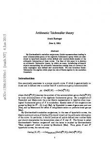
For a 3D surface, all the contours represent the ’shape’ of the surface. Inspired by the beautiful research work of Sharon and Mumford [27] on 2D shape analysis (recently it has been generalized to model multiple 2D contours [22]), we build a Teichm¨uller space for 3D shapes by using conformal mappings. In this Teichm¨uller space, every 3D contour (a simple closed curve) is represented by a point in the space; each point denotes a unique equivalence class of diffeomorphisms up to a M¨obius transformation. For a 3D surface, the diffeomorphisms of all the contours form a global shape representation of the surface. By using this signature, the similarities of 3D shapes can be quantitatively analyzed, therefore, the classification and recognition of 3D objects can be performed from their observed contours. We tested our algorithm in some segmented regions on a set of brain left cortical surfaces extracted from 3D anatomical brain MRI scans. The proposed method can reliably compute signatures on two cortical functional areas by computing the diffeomorphisms of each observed contour. Using the signature as the statistics, our method achieve about 92% accuracy rate to discriminate a set of AD subjects from healthy control subjects. To the best of our knowledge, it is the first work to apply contour diffeomorphism to brain morphometry research. Our experimental results demonstrated that this novel and simple method may be useful to analyze certain functional areas, and it may shed some lights on understanding detecting abnormality regions in brain surface morphometry. Our major contributions in this work include: 1. A new method to compute Teichm¨uller shape descriptor, in a way that generalized a prior 2D domain conformal mapping work [27]. 2. The method is theoretically rigorous and general. It presents a stable way to calculate the diffeomorphisms of contours in general 3D surfaces based on Ricci flow. 3. It involves solving elliptic partial differential equations (PDEs), so it is numerically efficient and computationally stable. 4. The shape descriptors are global and invariant to rigid motion and conformal deformations. Pipeline. Figure 1 shows the pipeline for computing the diffeomorphism signature for a surface with 3 closed contours. Here, we use a human brain hemisphere surface whose functional areas are divided and labeled in different color. The contours (simple closed curves) of functional areas can be used to slice the surface open to connected patches. As shown in frames (a-c), three contours γ1 , γ2 , γ3 are used to divide the whole brain (a genus zero surface S) to 4 patches S0 , S1 , S2 , S3 ; each of them is conformally mapped to a circle domain (e.g., disk or annuli), D0 , D1 , D2 , D3 . Note that γ1 is the contour of the joint functional areas of precuneus and posterior cingulate. One contour is mapped to two unit circles in two mappings. The representation of the shape according to each contour is a diffeomorphism of the unit circle to itself, defined as the mapping between periodic polar angles (Angle1 , Angle2 ), Angle1 , Angle2 ∈ [0, 2π]. The proper normalization is employed to remove M¨obius ambiguity. The diffeomorphisms induced by the conformal maps of each curve form a diffeomorphism signature, which is the Teichm¨uller coordinates in Teichm¨uller space. As shown in (d), the curves demonstrate the diffeomorphisms for three contours; the area distance is defined as the metric for shape comparison and classification.

4

Zeng, Shi, Wang and Gu

𝛾1 𝑐3 𝑐2

𝛾2 𝛾3 𝑐1 (a) contours on hemisphere brain surface

(b) conformal map of base domain D0

𝑆1 𝑆2 𝑆3

𝐷1

𝐷2 𝐷3 (c) conformal maps D1 , D2 , D3

(d) diffeomorphism signature

Fig. 1. Diffeomorphism signature via uniformization mapping for a genus zero surface with 3 simple closed contours γ1 , γ2 , γ3 in (a), which correspond to the boundaries c1 , c2 , c3 of the circle domains D1 , D2 , D3 in (c), respectively. These three contours are also mapped to the boundaries of the base circle domain D0 in (b). The curves in (d) demonstrate the diffeomorphisms for the three contours.

2

Theoretical Background

In this section, we briefly introduce the theoretical foundations necessary for the current work. For more details, we refer readers to the classical books [10, 16]. 2.1 Surface Uniformization Mapping Conformal mapping between two surfaces preserves angles. Suppose (S1 , g1 ) and (S2 , g2 ) are two surfaces embedded in R3 , g1 and g2 are the Euclidean induced Riemannian metrics. A mapping ϕ : S1 → S2 is called conformal, if the pull back metric of g2 induced by ϕ on S1 differs from g1 by a positive scalar function: ϕ∗ g2 = e2λ g1 , where λ : S1 → R is a scalar function, called the conformal factor. For example, all the conformal automorphisms of the unit disk form the M¨obius transformation group of the disk, each mapping is given by z − z0 . z → eiθ 1 − z¯0 z All the conformal automorphism group of the extended complex plane C ∪ {∞} is also called M¨obius transformation group, each mapping is given by z→

az + b , ad − bc = 1, a, b, d, c ∈ C. cz + d

Teichm¨uller Shape Descriptor and Its Application to Alzheimer’s Disease Study

5

By stereo-graphic projection, the unit sphere can be conformally mapped to the extended complex plane. Therefore, the M¨obius transformation group is also the conformal automorphism group of the unit sphere. A circle domain on the complex plane is the unit disk with circular holes. A circle domain can be conformally transformed to another circle domain by M¨obius transforz−z0 mations, z → eiθ 1−¯ z0 z . All genus zero surfaces with boundaries can be conformally mapped to circle domains: Theorem 21 (Uniformization) Suppose S is a genus zero Riemannian surface with boundaries, then S can be conformally mapped onto a circle domain. All such conformal mappings differ by a M¨obius transformation on the unit disk. This theorem can be proved using Ricci flow straightforwardly. Therefore, the conformal automorphism group of S Conf (S) is given Conf (S) := {ϕ−1 ◦ τ ◦ ϕ|τ ∈ M o¨b(S2 )}. ¨ 2.2 Teichmuller Space Definition 22 (Conformal Equivalence) Suppose (S1 , g1 ) and (S2 , g2 ) are two Riemannian surfaces. We say S1 and S2 are conformally equivalent if there is a conformal diffeomorphism between them. All Riemannian surfaces can be classified by the conformal equivalence relation. Each conformal equivalence class shares the same conformal invariants, the so-called conformal module. The conformal module is one of the key component for us to define the unique shape signature. ¨ Definition 23 (Teichmuller Space) Fixing the topology of the surfaces, all the conformal equivalence classes form a manifold, which is called the Teichm¨uller space. For example, all topological disks (genus zero Riemannian surfaces with single boundary) can be conformally mapped to the planar disk. Therefore, the Teichmuller space for topological disks consists of a single point. Suppose a genus zero Riemannian surface S has n boundary components {γ1 , γ2 , · · · , γn }, ∂S = γ1 + γ2 + · · · + γn , ϕ : S → D is the conformal mapping that maps S to a circle domain D, such that (a). ϕ(γ1 ) is the exterior boundary of the D; (b) ϕ(γ2 ) centers at the origin; (c) The center of ϕ(γ3 ) is on the imaginary axis. Then the conformal module of the surface S (also the circle domain D) is given by M od(S) = {(ci , ri )|i = 1, 2, · · · , n}. This shows the Teichm¨uller space of genus zero surfaces with n boundaries is of 3n − 6 dimensional. The Teichm¨uller space has a so-called Weil-Peterson metric [27], so it is a Riemannian manifold. Furthermore it is with negative sectional curvature, therefore, the geodesic between arbitrary two points is unique. 2.3 Surface Ricci Flow Surface Ricci flow is the powerful tool to compute uniformization. Ricci flow refers to the process of deforming Riemannian metric g proportional to the curvature, such that the curvature K evolves according to a heat diffusion process, eventually the curvature becomes constant everywhere. Suppose the metric g = (gij ) in local coordinate. Hamilton [15] introduced the Ricci flow as dgij = −Kgij . dt

6

Zeng, Shi, Wang and Gu

Surface Ricci flow conformally deforms the Riemannian metric, and converges to constant curvature metric [3]. Furthermore, Ricci flow can be used to compute the unique conformal Riemannian metric with the prescribed curvature. Theorem 24 (Hamilton and Chow [3]) Suppose S is a closed surface with a Riemannian metric. If the total area is preserved, the surface Ricci flow will converge to a Riemannian metric of constant Gaussian curvature.

2.4

¨ Teichmuller Shape Descriptor

Suppose Γ = {γ0 , γ1 , · · · , γn } is a set of non-intersecting smooth closed curves on a genus zero closed surface. Γ segments the surface to a set of connected components {Ω0 , Ω1 , · · · , Ωn }, each segment Ωi is a genus zero surface with boundary components. Construct the uniformization mapping ϕk : Ωk → Dk to map each segment Ωk to a circle domain Dk , 0 ≤ k ≤ n. Assume γi is the common boundary between Ωj and Ωk , then ϕj (γi ) is a circular boundary on the circle domain Dj , ϕk (γi ) is another 1 1 circle on Dk . Let fi |S1 := ϕj ◦ ϕ−1 k |S1 : S → S be the diffeomorphism from the circle to itself. We called the the diffeomorphism fi the signature of γi . Definition 25 (Signature of a Family of Loops) The signature of a family non-intersecting closed 3D curves Γ = {γ0 , γ1 , · · · , γk } on a genus zero closed surface is defined as: S(Γ ) := {f0 , f1 , · · · , fk } ∪ {M od(D0 ), M od(D1 ), · · · , M od(Dk )}. The following main theorem plays fundamental role for the current work. Note that if a circle domain Dk is disk, its conformal module can be omitted from the signature. Theorem 26 (Main Theorem) The family of smooth 3D closed curves Γ on a genus zero closed Riemannian surface is determined by its signature S(Γ ), unique up to a conformal automorphism of the surface η ∈ Conf (S). The proof of Theorem 26 can be found in the appendix section. The theorem states that the proposed signature determine shapes up to a M¨obius transformation. We can further do a normalization that fixes ∞ to ∞ and that the differential carries the real positive axis at ∞ to the real positive axis at ∞, as in Sharon and Mumford’s paper [27]. The signature can then determine the shapes uniquely up to translation and scaling. The shape signature S(Γ ) gives us a complete representation for the space of shapes. It inherits a natural metric. Given two shapes Γ1 and Γ2 . Let S(Γi ) := {f0i , f1i , · · · , fki }∪ {M od(Di0 ), M od(Di1 ), · · · , M od(Dik )} (i = 1, 2). We can define a metric d(S(Γ1 ), S(Γ2 )) between the two shape signatures using the natural metric in the Teichm¨uller space.Our signature is stable under geometric noise. Our algorithm depends on conformal maps from surfaces to circle domains using discrete Ricci flow method.

3

Algorithm

In this section, we explain each step of the pipeline in Figure 1 in details.

Teichm¨uller Shape Descriptor and Its Application to Alzheimer’s Disease Study

7

3.1 Circular Uniformization Mapping We apply discrete Ricci flow method [20] to conformally map the surfaces onto planar circle domains ϕk : Sk → D. The surface is represented as a triangle mesh Σ. A discrete Riemannian metric is represented as the edge length. We associate each vertex vi with a circle (vi , γi ), where γi is the radius. Let ui = log γi be the discrete conformal factor. The discrete Ricci flow is defined as follows: dui (t) ¯ i − Ki ), = (K dt

(1)

¯ i is the user defined target curvature and Ki is the curvature induced by the curwhere K rent metric. The discrete Ricci flow has exactly the same form as the smooth Ricci flow, which conformally deforms the discrete metric according to the Gaussian curvature. The computation is based on circle packing metric [20]. Suppose Σ is a genus zero mesh with multiple boundary components. The uniformization conformal mapping ϕ : Σ → D, where D is the circle domain, can be computed using Ricci flow by setting the prescribed curvature as follows: (a) The geodesic curvature on the exterior boundary is +1 everywhere; (b) the geodesic curvature on other boundaries are negative constants; (c) the Gaussian curvature on interior points are zeros everywhere. We use this method to compute conformal mapping, and get conformal module and shape descriptor. The main challenge is that the target curvature is dynamically determined by the metric. The metric is evolving, so is the target curvature. The detailed algorithm is reported in [38]. 3.2 Computing Shape Descriptor After the computation of the conformal mapping, each connected component is mapped to a circle domain. We define an order for all the loops on the surface, this induces an order for all the boundary components on each segment. Then by the definition for the conformal module of a circle domain, we normalize each circle domain using a M¨obius transformation, then compute the conformal modules directly. For those segments, which are simply connected and mapped to the unit disk, we compute its mass center, and use a M¨obius transformation to map the center to the origin. Each loop on the surface becomes the boundary components on two segments, both boundary components are mapped to a circle under the uniformization mapping. Then we compute the signature directly.

4

Experimental Results

We demonstrate the efficiency and efficacy of our method by analyzing the human brain cortexes of Alzheimer’s disease (AD) and healthy control subjects. The brain surfaces are represented as triangular meshes; a half brain with 100K triangles. We implement the algorithm using generic C++ on windows XP platform, with Intel Xeon CPU 3.39 GHz, 3.98 G RAM. The numerical systems are solved using Matlab C++ library. In general, the signature calculation on each half brain surface with 2 or 3 contours on each half takes less than 1 minute to compute, even on complicated domains. Data and preprocessing. The experimental data include 12 Alzheimer disease patients and 12 healthy control subjects. The structural MRI images were from the AD Neuroimaging Initiative (ADNI [19, 23]. We used Freesurfer’s automated processing

8

Zeng, Shi, Wang and Gu

𝛾2 right

𝛾2 left

𝛾1 right

𝛾1 left (a) superior view

(b) inferior view

(c) dlef t = 3.15022

(d) dright = −5.65014

Fig. 2. Diffeomorphisim signature (dlef t , dright ) of a healthy control brain cortex. Each (lef t and right) half brain is a genus zero surface with 2 contours.

pipeline [6] for automatic skull stripping, tissue classification, surface extraction, cortical and subcortical parcellations. It calculates volumes of individual grey matter parcellations in mm3 and surface area in mm2 . It also provides surface and volume statistics for about 34 different cortical structures, and also computes geometric characteristics such as curvature, curvedness, local foldedness for each of the parcellations [8]. In this work, we studied segmented surface regions for group difference analysis. Quantitative analysis. Figure 2 shows an example of diffeomorphism signatures for a brain cortical surface. We selected two contours on the left and the right half brain cortical surfaces, which correspond to superior temporal and the joint areas of precuneus and posterior cingulate. Early researches [17, 14] have indicated that these two areas may have significant atrophy in AD group. These two contours segment a brain hemisphere surface to 3 patches; one topological annulus (called the base domain), two topological disks. The base domain with two boundaries is mapped to an annulus, one boundary to exterior unit circle, the other one to the inner concentric circle. The diffeomorphism signature for each contour is plotted as a monotonic curve within the square [0, 2π] × [0, 2π]. The area difference between the plotted curves, ∫ 2π d = 0 (Angle22 − Angle12 )dAngle1 , is used as the metric to represent the global shape of both contours. So the signature of the whole brain surface is represented as a pair (dlef t , dright ) for combining the left-hemisphere and right-hemisphere brain shape signatures. The method was tested on 12 AD subjects and 12 healthy subjects,

Teichm¨uller Shape Descriptor and Its Application to Alzheimer’s Disease Study

9

Fig. 3. Distribution of diffeomorphism signature for 12 AD (in red) and 12 healthy control (CTL) (in blue) subjects. Each point denotes the diffeomorphism signature value (dlef t , dright ) for a whole brain surface, computed as in Figure 2.

with mean signatures (3.6827, −7.12957) and (5.2752, −5.6036), respectively. Figure 3 shows that with a simple linear discriminant analysis (LDA) model, there were only two subjects that were not correctly classified. It demonstrates that the proposed global diffeomorphism signature of contours is very efficient and may be effective to differentiate the shapes within healthy control and AD subject groups. Discussion. The proposed work is based on surface Ricci flow research. Computing the conformal module is equivalent to solving an elliptic partial differential equation on surfaces. According to PDE theory, the solution is smoother than its boundary conditions, so the solution process is quite stable. For surface-based AD research, the state-of-the-art work has used cortical thickness as the measurement [29, 5]. However, recent research [39] indicated that the commonly used cortical thickness and cortical area measurements are genetically and phenotypically independent. The biological meaning of the proposed shape signature is closely related to brain atrophy so it is more related to cortical area changes. Our method provides a unique and intrinsic shape feature to study brain morphometry changes caused by brain atrophy. It studies the sensitivity and reproducibility of shape features computed in the entire brain surface domain. The gained insights help improve our understanding to AD related pathology and discover the precise etiology of the grey matter changes. The preliminary results demonstrated that the shape signature provides a reasonably good discriminant power for AD biomarker research. We currently studied the superior temporal area, which is directly related to medial temporal lobe atrophy. The method can be equally applied to other regions as well. In future, we may study/compare other functional areas in the medial temporal lobe.

5

Conclusion

In this paper, we propose a novel method that computes the global shape signatures on specified functional areas on brain cortical surfaces in Teichm¨uller space. In the future,

10

Zeng, Shi, Wang and Gu

we will further explore and validate other applications of this global correlation shape signature in neuroimaging and shape analysis research.

References 1. S. Angenent, S. Haker, R. Kikinis, and A. Tannenbaum. Nondistorting flattening maps and the 3D visualization of colon CT images. IEEE Trans. Med. Imag., 19:665–671, 2000. 2. J. Ashburner, C. Hutton, R. Frackowiak, I. Johnsrude, C. Price, and K. Friston. Identifying global anatomical differences: deformation-based morphometry. Human Brain Mapping, 6:348–357, 1998. 3. B. Chow, P. Lu, and L. Ni. Hamilton’s Ricci Flow. American Mathematical Society, 2006. 4. M. K. Chung, K. M. Dalton, and R. J. Davidson. Tensor-based cortical surface morphometry via weighted spherical harmonic representation. IEEE Trans. Med. Imag., 27:1143–1151, 2008. 5. R. Cuingnet, E. Gerardin, J. Tessieras, G. Auzias, S. Lehricy, M.-O. Habert, M. Chupin, H. Benali, and O. Colliot. Automatic classification of patients with Alzheimer’s disease from structural MRI: A comparison of ten methods using the ADNI database. NeuroImage, 56(2):766 – 781, 2011. 6. A. M. Dale, B. Fischl, and M. I. Sereno. Cortical surface-based analysis I: segmentation and surface reconstruction. Neuroimage, 27:179–194, 1999. 7. R. H. Davies, C. J. Twining, P. D. Allen, T. F. Cootes, and C. J. Taylor. Shape discrimination in the hippocampus using an MDL model. in Proc. Infor. Proc. Med. Imag. (IPMI), 2003. 8. R. S. Desikan, F. Segonne, B. Fischl, B. T. Quinn, B. C. Dickerson, D. Blacker, R. L. Buckner, A. M. Dale, R. P. Maguire, B. T. Hyman, M. S. Albert, and R. J. Killiany. An automated labeling system for subdividing the human cerebral cortex on MRI scans into gyral based regions of interest. Neuroimage, 31:968–80, 2006. 9. B. Fischl, M. I. Sereno, and A. M. Dale. Cortical surface-based analysis II: Inflation, flattening, and a surface-based coordinate system. NeuroImage, 9:195 – 207, 1999. 10. F. P. Gardiner and N. Lakic. Quasiconformal Teichmuller theory. American Mathematical Society, 2000. 11. G. Gerig, M. Styner, D. Jones, D. Weinberger, and J. Lieberman. Shape analysis of brain ventricles using SPHARM. in Proc. MMBIA 2001, pages 171–178, 2001. 12. K. Gorczowski, M. Styner, J.-Y. Jeong, J. S. Marron, J. Piven, H. C. Hazlett, S. M. Pizer, and G. Gerig. Statistical shape analysis of multi-object complexes. IEEE Conf. Comp. Vis. Patt. Recog. CVPR ’07, pages 1–8, 2007. 13. X. Gu, Y. Wang, T. F. Chan, P. M. Thompson, and S.-T. Yau. Genus zero surface conformal mapping and its application to brain surface mapping. IEEE Trans. Med. Imag., 23:949–958, 2004. 14. X. Guo, Z. Wang, K. Li, Z. Li, Z. Qi, Z. Jin, L. Yao, and K. Chen. Voxel-based assessment of gray and white matter volumes in Alzheimer’s disease. Neurosci Lett, 468:146–50, 2010. 15. R. S. Hamilton. The Ricci flow on surfaces. Mathematics and general relativity, 71:237–262, 1988. 16. P. Henrici. Applied and Computational Complex Analysis, volume 3. Wiley-Intersecience, 1988. 17. X. Hua, S. Lee, D. P. Hibar, I. Yanovsky, A. D. Leow, A. W. Toga, C. R. J. Jr, M. A. Bernstein, E. M. Reiman, D. J. Harvey, J. Kornak, N. Schuff, G. E. Alexander, M. W. Weiner, and P. M. Thompson. Mapping Alzheimer’s disease progression in 1309 MRI scans: Power estimates for different inter-scan intervals. Neuroimage, 51:63–75, 2010. 18. M. K. Hurdal and K. Stephenson. Cortical cartography using the discrete conformal approach of circle packings. NeuroImage, 23:S119–S128, 2004. 19. C. R. J. Jack, M. A. Bernstein, N. C. Fox, P. M. Thompson, G. Alexander, D. Harvey, B. Borowski, P. J. Britson, J. L. Whitwell, C. Ward, and e. al. The Alzheimer’s disease neuroimaging initiative (ADNI): MRI methods. J. of Mag. Res. Ima., 27:685–691, 2007.

Teichm¨uller Shape Descriptor and Its Application to Alzheimer’s Disease Study

11

20. M. Jin, J. Kim, F. Luo, and X. Gu. Discrete surface Ricci flow. IEEE Trans. Vis. Comput. Graphics, 14:1030–1043, September 2008. 21. X. Liu, Y. Shi, I. Dinov, and W. Mio. A computational model of multidimensional shape. Int J Comput Vis, 89:69–83, 2010. 22. L. M. Lui, W. Zeng, S.-T. Yau, and X. Gu. Shape analysis of planar objects with arbitrary topologies using conformal geometry. In ECCV 2010, 2010. 23. S. G. Mueller, M. W. Weiner, L. J. Thal, R. C. Petersen, C. Jack, W. Jagust, J. Q. Trojanowski, A. W. Toga, and L. Beckett. The Alzheimer’s disease neuroimaging initiative. Neuroimaging clinics of North America, 15:869–877, 2005. 24. S. Pizer, D. Fritsch, P. Yushkevich, V. Johnson, and E. Chaney. Segmentation, registration, and measurement of shape variation via image object shape. IEEE Trans. Med. Imag., 18:851–865, 1999. 25. A. Qiu and M. I. Miller. Multi-structure network shape analysis via normal surface momentum maps. NeuroImage, 42:1430–8, 2008. 26. E. L. Schwartz, A. Shaw, and E. Wolfson. A numerical solution to the generalized Mapmaker’s problem: Flattening nonconvex polyhedral surfaces. IEEE Trans. Patt. Anal. Mach. Intell., 11:1005–1008, 1989. 27. E. Sharon and D. Mumford. 2D-shape analysis using conformal mapping. Int. J. Comput. Vision, 70:55–75, October 2006. 28. L. Shen, A. J. Saykin, M. K. Chung, and H. Huang. Morphometric analysis of hippocampal shape in mild cognitive impairment: An imaging genetics study. in IEEE 7th International Conference Bioinformatics and Bioengineering, 2007. 29. P. M. Thompson, K. M. Hayashi, G. D. Zubicaray, A. L. Janke, S. E. Rose, J. Semple, D. Herman, M. S. Hong, S. S. Dittmer, D. M. Doddrell, and A. W. Toga. Dynamics of gray matter loss in Alzheimer’s disease. J. Neuroscience, 23:994–1005, 2003. 30. P. M. Thompson and A. W. Toga. A surface-based technique for warping 3-dimensional images of the brain. IEEE Trans. Med. Imag., 15:1–16, 1996. 31. B. Timsari and R. M. Leahy. Optimization method for creating semi-isometric flat maps of the cerebral cortex. Medical Imaging 2000: Image Processing, 3979:698–708, 2000. 32. D. Tosun, A. Reiss, A. D. Lee, R. A. Dutton, K. M. Hayashi, U. Bellugi, A. M. Galaburda, J. R. Korenberg, D. L. Mills, A. W. Toga, and P. M. Thompson. Use of 3-D cortical morphometry for mapping increased cortical gyrification and complexity in Williams syndrome. Biom. Imag.: Nano to Macro, 2006. 3rd IEEE Int. Symp. on, 2006, pages 1172–1175, 2006. 33. A. Trouve and L. Younes. Metamorphoses through Lie group action. Foundations of Computational Mathematics, 5:173–198, 2005. 34. Y. Wang, X. Gu, T. F. Chan, and P. M. Thompson. Shape analysis with conformal invariants for multiply connected domains and its application to analyzing brain morphology. IEEE Conf. Comp. Vis. Patt. Recog. CVPR ’09, pages 202–209, 2009. 35. Y. Wang, X. Gu, T. F. Chan, P. M. Thompson, and S.-T. Yau. Brain surface conformal parameterization with algebraic functions. Med. Image Comp. Comput.-Assist. Intervention, Proceedings, Part II, pages 946–954, 2006. 36. Y. Wang, X. Gu, T. F. Chan, P. M. Thompson, and S.-T. Yau. Conformal slit mapping and its applications to brain surface parameterization. Med. Image Comp. Comput.-Assist. Intervention, Proceedings, Part I, pages 585–593, 2008. 37. Y. Wang, L. Lui, X. Gu, K. M. Hayashi, T. F. Chan, A. W. Toga, P. M. Thompson, and S.T. Yau. Brain surface conformal parameterization using Riemann surface structure. IEEE Trans. Med. Imag., 26:853–865, 2007. 38. Y. Wang, J. Shi, X. Yin, X. Gu, T. F. Chan, S.-T. Yau, A. W. Toga, and P. M. Thompson. Brain surface conformal parameterization with the Ricci flow. submitted to IEEE Trans. Med. Imag., 2011. 39. A. M. Winkler, P. Kochunov, J. Blangero, L. Almasy, K. Zilles, P. T. Fox, R. Duggirala, and D. C. Glahn. Cortical thickness or grey matter volume? The importance of selecting the phenotype for imaging genetics studies. NeuroImage, 53(3):1135 – 1146, 2010.

12

Zeng, Shi, Wang and Gu Ω0

𝛾3 Ω4

Ω1 Ω2

Ω1 𝛾1

Ω3 𝛾2 𝛾5 Ω 6

Ω2 𝛾3

𝛾1 Ω5 𝛾4 𝛾0

Ω4

𝛾4

𝑆

Φ0 : Ω0 → 𝐷0

Ω0 𝛾0

Ω

𝛾0, 𝑓01 Φ1 : Ω1 → 𝐷1 𝛾1, 𝑓12

𝛾2

Φ 2 : Ω 2 → 𝐷2

Ω3 𝛾5

Ω5

𝛾3, 𝑓24

Ω6

Φ4 : Ω4 → 𝐷4

𝑆0

𝑆1 𝑆3

𝛾2, 𝑓13 Φ3 : Ω3 → 𝐷3 𝛾4, 𝑓25

Φ5 : Ω5 → 𝐷5

𝛾5, 𝑓36

𝑆2

𝑆6

𝑆4 𝑆5

Φ6 : Ω6 → 𝐷6

Fig. 4. Proof for the main theorem, the signature uniquely determines the family of closed curves ¨ unique up to a Mboius transformation.

Appendix: Proof of Theorem 26 proof See Figure 4. In the left frame, a family of planar smooth curves Γ = {γ0 , · · · , γ5 } divide the plane to segments {Ω0 , Ω1 , · · · , Ω6 }, where Ω0 contains the ∞ point. We represent the segments and the curves as a tree in the second frame, where each node represents a segment Ωk , each link represents a curve γi . If Ωj is included by Ωi , and Ωi and Ωj shares a curve γk , then the link γk in the tree connects Ωj to Ωi , denoted as γk : Ωi → Ωj . In the third frame, each segment Ωk is mapped conformally to a circle domain Dk by Φk . The signature for each closed curve γk is computed fij = Φi ◦ Φ−1 j |γk , where γk : Ωi → Ωj in the tree. In the last frame, we construct a Riemann sphere by gluing circle domains Dk ’s using fij ’s in the following way. The gluing process is of bottom up. We first glue the leaf nodes to their fathers. Let γk : Di → Dj , Dj be a leaf of the tree. For each point z = reiθ in Dj , the extension map: Gij (reiθ ) = refij (θ) . We denote the image of Dj under Gij as Sj . Then we glue Sj with Di . By repeating this gluing procedure bottom up, we glue all leafs to their fathers. Then we prune all leaves from the tree. Then we glue all the leaves of the new tree, and prune again. By repeating this procedure, eventually, we get a tree with only the root node, then we get a Riemann sphere, denoted as S. Each circle domain Dk is mapped to a segment Sk in the last frame, by a sequence of extension maps. Suppose Dk is a circle domain, a path from the root D0 to Dk is {i0 = 0, i1 , i2 , · · · , in = k}, then the map from Gk : Dk → Sk is given by: Gk = Gi0 i1 ◦ Gi1 i2 ◦ · · · ◦ Gin−1 in . Note that, G0 is identity. Then the Beltrami coefficient of G−1 k : Sk → Dk can be directly computed, denoted as µk : Sk → C. The composition Φk ◦ G−1 : Sk → Ωk maps Sk to Ωk , k because Φk is conformal, therefore the Beltrami coefficient of Φk ◦ G−1 k equals to µk . We want to find a map from the Riemann sphere S to the original Riemann sphere Ω, Φ : S → Ω. The Beltrami-coefficient µ : S → C is the union of µk ’s each segments: µ(z) = µk (z), ∀z ∈ Sk . The solution exists and is unique up to a M¨obius transformation according to Quasi-conformal Mapping theorem [10]. Note that, the discrete computational method is more direct without explicitly solving the Beltrami equation. From the Beltrami coefficient µ, one can deform the conformal structure of Sk to that of Ωk , under the conformal structures of Ωk , Φ : S → Ω becomes a conformal mapping. The conformal structure of Ωk is equivalent to that of Dk , therefore, one can use the conformal structure of Dk directly. In discrete case, the conformal structure is represented as the angle structure. Therefore in our algorithm, we copy the angle structures of Dk ’s to S, and compute the conformal map Φ directly.