Oct 24, 2011 - [102] Karin Stenderup, Jeannette Justesen, Christian Clausen, and Moustapha. Kassem. Aging is associated with decreased maximal life span ...
N ◦ d'ordre
: 4335
THÈSE PRÉSENTÉE À
L'UNIVERSITÉ BORDEAUX I ÉCOLE DOCTORALE DE MATHÉMATIQUES ET D'INFORMATIQUE
tel-00635273, version 1 - 24 Oct 2011
Par
Rodrigo ASSAR
CUEVAS
POUR OBTENIR LE GRADE DE
DOCTEUR SPÉCIALITÉ :
INFORMATIQUE
Modeling and simulation of Hybrid Systems and Cell factory applications Soutenue le :
21 Octobre 2011
Après avis des rapporteurs : Jean-Michel Couvreur
Professeur
Servet Martínez . . . . .
Director de Recherche
Devant la commission d'examen composée de : Jean-Michel Couvreur
Professeur . . . . . . . . . . . . . . . . . . .
Président de jury
Alain Gri�ault . . . . . . .
Maître de Conférences . . . . . . .
Rapporteur
Servet Martínez . . . . .
Director de Recherche . . . . . . .
Rapporteur
David J. Sherman . . .
Professeur . . . . . . . . . . . . . . . . . . .
Directeur de Thèse
� 2011 �
tel-00635273, version 1 - 24 Oct 2011
Acknowledgments Firstly, I would like to thank my director of thesis, Professor David Sherman for their guidance, patience and outstanding support throughout my doctoral studies. I would also like to extend my gratitude to all the MAGNOME team of the LaBRI, who helped me to learn important lessons of life. The INRIA is gratefully acknowledged for �nancially supporting my studies in France on a CORDI-S fellowship. Thanks to all the jury: Servet Martínez and Jean-Michel Couvreur who reviewed my thesis, and Alain Gri�ault who gentily has taken part of the jury. I want to �nish by thanking to my family, my parents and Coté, who have supported and encouraged me throughout my PhD studies. I dedicate this thesis to
tel-00635273, version 1 - 24 Oct 2011
them.
tel-00635273, version 1 - 24 Oct 2011
Modeling and simulation of Hybrid Systems and Cell factory applications Abstract :
The main aim of this thesis is to develop an approach that allows
us to describe biological systems with theoretical sustenance and good results in practice. Biological functions are the result of the interaction of many processes, that connect di�erent hierarchy levels going from macroscopic to microscopic level. Each process works in di�erent way, with its own goal, complexity and hierarchy level. In addition, it is common to observe that changes in the conditions, such as nutrients or environment, modify the behavior of the systems. So, to describe the behavior of a biological system over time, it is convenient to combine di�erent types of models:
tel-00635273, version 1 - 24 Oct 2011
continuous models for gradual changes, discrete models for instantaneous changes, deterministic models for completely predictable behaviors, and stochastic or nondeterministic models to describe behaviors with imprecise or incomplete information. In this thesis we use the theory of Composition and Hybrid Systems as basis, and the BioRica framework as tool to model biological systems and analyze their emergent properties
in silico.
With respect to Hybrid Systems, we considered continuous models given by sets of di�erential equations or more general dynamics. We used Stochastic Transition
coe�cient switches strong switches that choose
Systems to describe the dynamics of model changes, allowing that control the parameters of the continuous model, and
di�erent models. Composition, reconciliation and reusing of models allow us to build complete and consistent descriptions of complex biological systems by combining them. Compositions of hybrid systems are hybrid systems, and the re�nement of a model forming part of a composed system results in a re�nement of the composed system.
To implement our approach ideas we complemented the theory of our
approach with the improving of the BioRica framework. We contributed to do that giving a BioRica speci�cation of Hybrid Systems that assures integrity of models, allowing composition, reconciliation, and reuse of models with SBML speci�cation. We applied our approach to describe two systems: wine fermentation kinetics, and cell fate decisions leading to bone and fat formation.
In the case of wine
fermentation, we reused known models that describe the responses of yeasts cells to di�erent temperatures, quantities of resources and toxins, and we reconciled these models choosing the model with best adjustment to experimental data depending on the initial conditions and fermentation variable. The resulting model can be applied to avoid process problems as stuck and sluggish fermentations. With respect to cell fate decisions the idea is very ambitious.
By using accurate models to predict
the bone and fat formation in response to activation of pathways such as the Wnt pathway, and changes of conditions a�ecting these functions such as increments in Homocysteine, one can analyze the responses to treatments for osteoporosis and other bone mass disorders. We think that here we are giving a �rst step to obtain
in silico
evaluations of medical treatments before testing them
in vitro
or
in vivo.
Keywords :
Biological systems, hybrid systems, composition, reusing and recon-
ciling models, BioRica, wine fermentation kinetics, bone formation.
Discipline :
Computer-Science
LaBRI Université Bordeaux 1 351 cours de la Libération,
tel-00635273, version 1 - 24 Oct 2011
33405 Talence Cedex (FRANCE)
tel-00635273, version 1 - 24 Oct 2011
Résumé :
Les Fonctions biologiques sont le résultat de l'interaction de beaucoup de
processus, avec di�erents objectives, complexités, niveaux d'hiérarchie, et changements de conditions que modi�ent le comportement de systèmes.
Nous utilisons
des équations diferenciales ou dynamiques plus générales, et Stochastic Systèmes de Transition pour décrire la dynamique de changements des modèles. La composition, réconciliation et reutilisation des modèles nous permettent d'obtenir des descriptions de systèmes biologiques complètes et compatibles et leur combiner. Notre spéci�cation de Systèmes Hybrides avec BioRica assures l'intégrité de modèles, et implement notre approche. Nous appliquons notre approche pour décrire in-silico deux systèmes: la dynamique de la fermentation du vin, et des décisions cellulaires associées à la formation de tissu d'os.
Mots clefs :
Systèmes biologiques, Systèmes hybrides, composition, réconcilia-
tion et reutilisation des modèles, BioRica, dynamique de la fermentation du vin,
tel-00635273, version 1 - 24 Oct 2011
formation de tissu d'os.
Discipline :
Informatique
LaBRI Université Bordeaux 1 351 cours de la Libération, 33405 Talence Cedex (FRANCE)
tel-00635273, version 1 - 24 Oct 2011
Contents Contents
1
List of Figures
4
1 Introduction
11
1.1
1.2
Dynamical Models for Biological Systems . . . . . . . . . . . . . . . . 1.1.1
Fitting biological models . . . . . . . . . . . . . . . . . . . . .
13
1.1.2
Model speci�cations
15
. . . . . . . . . . . . . . . . . . . . . . .
Composition and Hierarchy challenges
. . . . . . . . . . . . . . . . .
Modularity and Hierarchy of biological systems
. . . . . . . .
16
1.2.2
Sti�ness and timescales . . . . . . . . . . . . . . . . . . . . . .
18
1.2.3
Composition: its challenges
18
. . . . . . . . . . . . . . . . . . .
Presence of randomness and use of Hybrid Systems in Biology
1.4
Outline of this thesis
. . . .
19
. . . . . . . . . . . . . . . . . . . . . . . . . . .
20
2 Preliminaries
2.2
2.3
16
1.2.1
1.3
2.1
11
23
Hybrid Systems . . . . . . . . . . . . . . . . . . . . . . . . . . . . . .
23
2.1.1
Continuous dynamics . . . . . . . . . . . . . . . . . . . . . . .
24
2.1.2
Discrete dynamics . . . . . . . . . . . . . . . . . . . . . . . . .
26
2.1.3
Interactions between continuous and discrete dynamics
. . . .
26
2.1.4
Switched Systems . . . . . . . . . . . . . . . . . . . . . . . . .
26
Stochastic Transition Systems
. . . . . . . . . . . . . . . . . . . . . . . . . . . . . . . . . . . . .
27
2.2.1
Randomness and non-determinism
2.2.2
Dynamics of system variables: Probabilistic modules
2.2.3
Inclusion of Time: Continuous-Time Markov Decision Process
2.2.4
Schedulers and Timed executions
2.2.5
Extensions of Stochastic Transition Systems
. . . . . . . . . .
34
2.2.6
Measurability of schedulers and executions . . . . . . . . . . .
37
Composition of models . . . . . . . . . . . . . . . . . . . . . . . . . .
39
2.3.1
Composition of probabilistic modules . . . . . . . . . . . . . .
39
2.3.2
Input-output connections . . . . . . . . . . . . . . . . . . . . .
43
. . . . .
. . . . . . . . . . . . . . . .
3 Our approach: Modeling biological systems
29 30 32 33
45
3.1
Reusing and reconciling models by composition
. . . . . . . . . . . .
45
3.2
Modeling biological systems as Hybrid systems . . . . . . . . . . . . .
46
3.3
Describing hybrid systems
47
. . . . . . . . . . . . . . . . . . . . . . . .
1
Contents 3.3.1
Formalization . . . . . . . . . . . . . . . . . . . . . . . . . . .
3.3.2
Two types of hybrid systems: with strong switches
with coe�cient switches and
. . . . . . . . . . . . . . . . . . . . . . .
48
3.4
Guarantees
. . . . . . . . . . . . . . . . . . . . . . . . . . . . . . . .
50
3.5
General contributions . . . . . . . . . . . . . . . . . . . . . . . . . . .
51
4 Our implementation: Simulating biological systems Requirements of the implementation
. . . . . . . . . . . . . . . . . .
53
4.2
Solving hybrid systems . . . . . . . . . . . . . . . . . . . . . . . . . .
54
4.3
Improving the BioRica framework for simulating biological systems
.
55
4.3.1
The BioRica prototype . . . . . . . . . . . . . . . . . . . . . .
55
4.3.2
Improving BioRica
56
4.5
tel-00635273, version 1 - 24 Oct 2011
53
4.1
4.4
. . . . . . . . . . . . . . . . . . . . . . . .
Implementing and simulating hybrid systems with BioRica
. . . . . .
57
4.4.1
Syntax and semantics of BioRica for hybrid systems . . . . . .
57
4.4.2
Simulations
. . . . . . . . . . . . . . . . . . . . . . . . . . . .
60
Conclusion . . . . . . . . . . . . . . . . . . . . . . . . . . . . . . . . .
61
5 Application: Reconciling competing models, particular case of wine fermentation kinetics . . . . . . . . . . . . . . . . . .
63
5.1
Modeling wine fermentation kinetics
5.2
Experimental data and exploratory analysis
5.3
Statistical classi�cation of the results
5.4
Reconciled model of wine fermentation kinetics
. . . . . . . . . . . .
71
5.5
Results . . . . . . . . . . . . . . . . . . . . . . . . . . . . . . . . . . .
74
5.6
63
. . . . . . . . . . . . . .
65
. . . . . . . . . . . . . . . . . .
70
5.5.1
Reconciled models and simulations
. . . . . . . . . . . . . . .
74
5.5.2
Detecting sluggish and stuck fermentations . . . . . . . . . . .
78
Conclusions and discussion . . . . . . . . . . . . . . . . . . . . . . . .
79
6 Application: modeling cell fate, particular case of bone precursors di�erentiation
81
6.1
Mechanisms of regulation . . . . . . . . . . . . . . . . . . . . . . . . .
6.2
Gene Regulatory Networks and Switched Systems . . . . . . . . . . .
83
6.3
Approach
84
6.4
2
48
. . . . . . . . . . . . . . . . . . . . . . . . . . . . . . . . .
82
6.3.1
Reused models
. . . . . . . . . . . . . . . . . . . . . . . . . .
85
6.3.2
The main osteo-adipo switch model . . . . . . . . . . . . . . .
86
6.3.3
The osteo-adipo switch model: including the Wnt pathway as a stimulus for bone cell di�erentiation . . . . . . . . . . . . . .
86
6.3.4
Composing models
. . . . . . . . . . . . . . . . . . . . . . . .
87
6.3.5
Adjusting the model to human cells . . . . . . . . . . . . . . .
89
Results . . . . . . . . . . . . . . . . . . . . . . . . . . . . . . . . . . .
89
6.4.1
Cell division . . . . . . . . . . . . . . . . . . . . . . . . . . . .
89
6.4.2
Cell di�erentiation
90
6.4.3
Consolidated models
. . . . . . . . . . . . . . . . . . . . . . . . . . . . . . . . . . . . . . . . . . . . . . .
93
6.5
Conclusions and discussion . . . . . . . . . . . . . . . . . . . . . . . .
93
6.6
Other cell division and di�erentiation models . . . . . . . . . . . . . .
95
6.6.1
95
Regulation of cell division by Goldbeter model . . . . . . . . .
6.6.2
Cell di�erentiation of blood cells . . . . . . . . . . . . . . . . .
7 Conclusions and discussion
99
7.1
Conclusions
7.2
Future work . . . . . . . . . . . . . . . . . . . . . . . . . . . . . . . . 101
99
105
tel-00635273, version 1 - 24 Oct 2011
Bibliography
. . . . . . . . . . . . . . . . . . . . . . . . . . . . . . . .
96
3
List of Figures 1.1
Guyton model [46]. The system is composed by 18 interconnected modules, each one modeling a di�erent function associated with the human circulatory physiology. Systems of di�erential equations, DAEs and other models are used in each module. . . . . . . . . . . . . . . . . . . . . . . .
tel-00635273, version 1 - 24 Oct 2011
2.1
A) :
The dynamics of a
Switched System.
17
The model moves between
di�erent modes, nodes in the picture, de�ning its discrete dynamics. At each mode, the system changes its continuous dynamics.
Switched System of the motion of a car.
The
The continuous dynamics, repre-
sented by the evolution of the variables position its laws according to the engaged gear. 2.2
B) :
s and velocity v , changes
. . . . . . . . . . . . . . . . . .
27
Example of Transition system for cell division. Circles represent states, black arrows transitions. Transitions are labeled by actions, but di�erent transitions can have the same label to represent that an action may produce many responses.
The initial action selects the initial state of
q0 . States: q0 , q1 , q2 , transitions: (q0 , s, q0 ), (q1 , e, q2 ). Red arrows are inherent idle transi-
the system, always begin at
(q0 , a, q1 ), (q1 , e, q0 )
and
tions that are added to the system to assure in�nite executions, and to de�ne composition. . . . . . . . . . . . . . . . . . . . . . . . . . . . . . . 2.3
Example of Stochastic transition system. (two possible successors of
q1
29
The presence of randomness
e: q0
under the action
and
q2 )
and the
time advance are modeled by considering that spent time of transitions has exponential distribution. We show the rate values between parenthesis.
2.4
q0 ),
can be solved by a
that assigns them probabilities. . . . . . . . . . . .
q1
two actions,
a
or
b.
. . . . . . . . . . .
of our old example (Figure 2.2) was decomposed into two actions ∗ and e1 . The action e0 has an in�nity of possible transitions: any q
{{A = 1, N = 1, G ∈ [0, 1]}
with G given byµ}.
e0 ∈
. . . . . . . . . . . . . .
36
Stochastic transition system that represents the behavior of G (growth of cell). It is formed by the states:
g0 , g1
and
g2 .
with the same probability any state, the action
4
35
Stochastic Transition system with continuous space of states. The action
e
2.6
34
Stochastic Transition system with inclusion of rate values for spent times (between parenthesis). At state
2.5
at each arrow
The non-determinism, associated to have two or
more actions possible at the same state (case of
randomized scheduler
R
The initial action selects
g
relates the states.
. . .
40
List of Figures 2.7
Two
Transition systems
that at composing them represents the cell di-
vision process as depending on a growth index. Extension of models of Figure 2.2 and 2.6. We do not show the idle transitions at each state. . . 2.8
42
Guyton model [46] restricted to the renin-angiotensin-aldosterone system. Systems of di�erential equations, DAEs and other models are used in each module, and they are connected by input-output relations. Rates
M DF LW (�uid in the renal tubules at macula densa), T V D N OD, KOD, V U D (urine output), ADH (rate of hormone entry into the �uids). Concentrations: CKE , CN A, ADHC (antidiuretic hormone in the blood). Multiplier e�ects: AN M (angiotensin), AM K , AM N A, ADHM K . . . . . . . . . . . . . . . . . . . . . . . . . variables:
(�uid intake),
3.1
.
44
to chose the best one in function of factor conditions. . . . . . . . . . . .
46
Reconciliation process. First we have the original models, then we control
tel-00635273, version 1 - 24 Oct 2011
them to run them in parallel, �nally we control the selection of models
3.2
Modeling schema of Complex Biological Systems using Hybrid models. First one identi�es the discrete and continuous interacting dynamics, then one separates the continuous dynamics into two interacting models: the
3.3
X MODEL that describes the dynamics of X , and the residual model.
Abstraction of Hybrid systems. (A) The module
X MODEL
47
describes
x. It interacts with two other modules: CON T ROL and M ODE . CON T ROL computes the values of the continuous control variables u, M ODE decides the valthe continuous model of the state variables
ues of the mode variables.
Arrows denote input-output relations.
(B)
N models. The j−th model is represented by its continuous dynamics M odel j , that interacts with two modules: the controller CON T ROLj , and M ODE j that decides if the model is active Strong switches between
or not. . . . . . . . . . . . . . . . . . . . . . . . . . . . . . . . . . . . . . 3.4
Abstraction of the reconciliation of models as hybrid system with strong switches.
4.1
49
The
j−th
model is represented by its continuous dynamics
M odel j , that and M ODES
that decides if the model is active or not by means of the
mode variable
mode j .
interacts with two modules: the controller
CON T ROLj ,
. . . . . . . . . . . . . . . . . . . . . . . . . . . .
50
Computation steps to solve an hybrid system, options used for wine fermentation shown in red. conditions
IC
The process begins reading inputs: initial
and parameters values
P.
It is initialized the time in
and computed the initial values of the mode variables. tains the initial de�nition of the model
0,
Then, one ob-
M ODEL(mode(0)).
At any time
the model is solved, it is updated when detecting the guard condition
GU ARD(x, mode, u, time), and EN D(x, mode, u, time). . . . .
the process �nishes when it is veri�ed . . . . . . . . . . . . . . . . . . . . . . .
55
5
List of Figures 4.2
Implementation of hybrid systems with BioRica. (A) The node
X
de-
x. It interacts with M ODE . CON T ROL computes the values of the continuous control variables u, M ODE decides the values of the mode variables. The node M AIN de�nes their interactions. (B) Strong switches between N continuous models. The j−th model is described by the node M j , that interacts with two modules: the controller CON T ROLj , and M ODEj that decides if the model is active or not. The node M AIN de�nes their interactions. . . . . . . . . . . . . . scribes the continuous model of the state variables
two other modules:
4.3
tel-00635273, version 1 - 24 Oct 2011
and
.
58
. . . . . . . . . . . . . . . . . . . . . . . . . . . . . . . . . . .
59
The radiator. (A)Schema of the Hybrid system. (B)Three models. (B.1) ◦ deterministic: it is turned on if the temperature T is lower than 18 C and ◦ turned o� if it is bigger than 20 C , (B.2) non-deterministic: both events 2 to can happen if 18 6 T 6 20, and (B.3) stochastic giving probability 3 turn on. (C)Evolution of the temperature for the model (B.1), and (D) for (B.3).
4.4
CON T ROL
(A) Diagram of a Zeno's water tank. (B) Switched model of the behavior. (C) BioRica code and (D) Simulation.
The rule to decide into which
tank water must be sent considers that the water level of tank
1
must
r1 and that the tank 2 higher than r2 . At x1 and x2, r1 = r2 = 2, the simulations run an increasing number of transitions to try to verify x1 > r1 and x2 > r2. . . . . . . . . .
be higher than arriving to mode
5.1
.
60
linear correlations in transient phase of 0.98, 0.99 and 0.97 respectively. .
68
Fermentation variables pro�les for some initial conditions con�gurations. For Biomass and Sugar one shows experimental results in LHH (low ◦ temperature: 12 C , high initial sugar: 268 g/l , high initial nitrogen: 300 mg/l), HM M (28◦ C , sugar: 238 g/l, nitrogen: 50mg/l) and HM H (28 ◦ C , sugar: 233 g/l, nitrogen: 300 mg/l) con�gurations. For Ethanol we ◦ show data for M M M con�guration (20 C , sugar: 200 g/l , nitrogen: 66
mg/l) instead of LHH . 5.2
Log-Biomass pro�les are shown too, we obtained
Summary of results of adjustment according to initial conditions. Quality of adjustment of each model for each initial conditions con�guration and phase (transient and stable). . . . . . . . . . . . . . . . . . . . . . . . . .
5.3
71
Reconciled model of wine kinetics for con�guration M HH : temperature 23◦ C , sugar 308.6[g/l], and nitrogen 275[mg/l]. (A)Codes: MODEL describes the continuous part, MODES decides if the mode associated to Scaglia (mode_S ) or the associated to Coleman (mode_C ) is active, and RECONCILED MODEL OF SUGAR CONFIG MHH combines the results of the active models at each time. The change from transient to stable phase, triggered by a su�ciently low concentration of sugar and high concentrations of biomass and ethanol, is modeled to happen at time given by a gaussian variable with mean standard deviation tration.
6
sd_M HH = 18.55
T T ime_M HH = 121
and
(B)Simulation of sugar concen-
. . . . . . . . . . . . . . . . . . . . . . . . . . . . . . . . . . . .
75
List of Figures 5.4
Reconciled
model
of
wine
kinetics for ◦ 34 C , sugar
high
initial
condi-
HHH : temperature 245.45[g/l], and ni280[mg/l]. (A)Codes: One BioRica node per original model, M ODES decides if each model is active or not, and RECON CILED_M ODEL_OF _SU GAR_CON F IG_HHH
tions
trogen
combines the results of the active models at each time.
The change
from transient to stable phase, triggered by a su�ciently low concentration of sugar and high concentrations of biomass and ethanol, is modeled to happen at time given by a a gaussian variable with mean
T T ime_HHH = 105.5
and standard deviation
sd_HHH = 19.125.
(B)Simulation of sugar concentration. . . . . . . . . . . . . . . . . . . . .
6.1
The osteo-chondro switch di�erentiation model by [96]. The expression
RUNX2
of two mutually exclusive genes (
the bone and cartilage formation,
tel-00635273, version 1 - 24 Oct 2011
77
SOX9 ) is associated with respectively. The gene Tweak is the and
bio-marker for the progenitor state. Initially, an unknown stimuli that favors bone or cartilage formation is considered. Then, the outcomes are modeled by stochastic switches in the coe�cients values of the model. . . 6.2
Osteo-adipo switch di�erentiation model.
RUNX2
tually inhibiting genes (
and
85
The expressions of two mu-
P P ARγ )
are associated to the os-
teoblast and adipocyte lineage decision respectively, and a third bio-
OCT4
marker (
or
SOX2 )
detects osteo-adipo progenitor cells.
canonical Wnt pathway is active, stimulated by lithium, to the nucleus of the cell and promotes the expression of favors the bone formation. The activation of the formation of adipocytes. 6.3
If the
β−catenin
goes
RUNX2, which
P P ARγ
stimulates the
. . . . . . . . . . . . . . . . . . . . . . . . . . .
87
Composed model of cell fate. A progenitor cell can divide into new progenitor cells, or can die (apoptosis), or can di�erentiate into more speci�c lineages. Each one of these possibilities is controlled by a regulatory system. Apoptosis is stimulated by inducers, here quanti�ed by increases of
Hcy protein.
Division is induced if the cell carries a su�ciently high level
of maturation (called
MP F ,
[108] model). Di�erentiation is stimulated
by inhibitions of the progenitor maintenance role (associated to speci�c genes), after which that the cell decides its lineage. Each speci�c lineage is stimulated by signals: the activation of the canonical Wnt pathway (model in [62]) stimulates bone formation (osteoblast lineage), and the pathway of 6.4
P P ARγ
the formation of fat (adipocyte lineage).
. . . . . .
88
BioRica code and simulation of [108] model of regulation of cell division. Code is obtained from SBML models. Cell mitosis are predicted to happen when the maturation promoting factor reaches its threshold.
Total
cyclin yt
concentrations with respect to the total di�erence between two divisions.
and
M
MPF
(variable
M)
are expressed as relative
cdc2 CT .
Period is the temporal
. . . . . . . . . . . . . . . . . . . . . .
89
7
List of Figures 6.5
BioRica code and simulations of the osteo-chondro switch di�erentiation model in [96]). Stimuli are included by a probabilistic scenario externally
D.xp denotes the concentration of the progenitor biothe osteoblast lineage and D.xc of the chondrocytes
modeled. Variable marker, lineage.
D.xo
of
The pro-di�erentiation stimulus happens at time exponential
with expected value
t = 100
minutes, the pro-osteogenic stimulus hap-
t = 500 minutes, and the value t = 1000 minutes. . . .
pens at time exponential with expected value pro-chondrogenic stimulus with expected
6.6
.
90
. . . . . . . . . . . . . . . . . . . . . .
91
BioRica code and simulations of our osteo-adipo switch model.
DIFF xA .
is the same of the osteo-chondro switch model, replacing
Node
xC
by
The activation of the canonical Wnt pathway (model by [62]) is a
P P ARγ
stimulus to the osteoblast lineage, The activation of the
path-
way, stimulates the adipocyte lineage, and it is simulated by an expo-
tel-00635273, version 1 - 24 Oct 2011
nential probability distribution with mean
1000
minutes. In case of Wnt
activation, the pro-osteoblast di�erentiation coe�cient
0.8. 6.7
For
P P ARγ
it increases
zA .
zO
increases to
The cell fate decisions model: composed model of cell fate for osteo-adipo progenitor cells. Boxes and circles represent models here used, coded by BioRica nodes. Edges represent input-output relations. The
ENTIATION MODEL
de�nes the dynamics of
xP , xO
and
DIFFER-
xA
ing progenitors, osteoblasts, and adipocytes respectively. The
describ-
STIMULI
MODEL de�nes the transitions of the di�erentiation model by giving the update values to DIFFERENTIATION MODEL. The models in circles represent the models to regulate division and apoptosis. precursor and osteoblast cells is stimulated by increasing exponential time with mean
2000
Apoptosis of
Hcy
([63]) at
minutes. Division happens if the cell
carries the maximal level of maturation, maximizing
M
([108]). Di�er-
entiation is simulated to happen after an exponential time with mean
100
minutes.
The activation of the canonical Wnt pathway (model in
[62]) stimulates osteoblast lineage in the period the activation of the pathway of distribution of mean
P P ARγ
500 − 1000 minutes,
and
(simulated by an exponential
1000 minutes) the adipocyte lineage.
In simulations
we show the percentages of each type of cells with respect with the initial quantity of progenitors. . . . . . . . . . . . . . . . . . . . . . . . . . . . .
6.8
92
BioRica codes and simulations of the Goldbeter model ([40]) of regulation of cell division. (A) The Goldbeter model. (B) The Goldbeter model sim+ pli�ed by piecewise-a�ne approximations of Hill functions (h (C, Kd , 1) θ + and h (C, Kc , 1) are the original ones) by using the thresholds θ1 = 5 9θ and θ2 = . Cell mitosis are predicted to happen each time that the 5 variable M (concentration of the maturation promoting factor )
MPF
reaches the threshold value. The observed period between mitosis is
25
minutes approximately. . . . . . . . . . . . . . . . . . . . . . . . . . . . .
8
95
List of Figures 6.9
BioRica code and simulations of an red-white blood cells di�erentiation model in [55]). The pro-di�erentiation stimuli for each cell lineage (red and white blood cells) are modeled by considering the auto-stimulation
λ di�er. In case (A) both values are equal λR = λW = 0.5, in (B) λR = 0.5 and λw = 0.7, and in (C) λR = 0.7 and λw = 0.5. Parameters are n = 4, kR = kW = bR = bW = 1, and the θ's coe�cients have value 0.5. As in [55], we show the relative quantities of xR (GAT A1) and xW (P U.1) coe�cients as functions over time whose rate of exponential decrease
. . . . . . . . . . . . . . . . . . . . . . . . . . . . . . . . . . .
97
tel-00635273, version 1 - 24 Oct 2011
over time.
9
10
tel-00635273, version 1 - 24 Oct 2011
Chapter 1 Introduction The aim of this chapter is to present the main elements for modeling biological
tel-00635273, version 1 - 24 Oct 2011
systems.
We summarize about the challenges to model this type of systems, the
methodology and speci�cations. The main points that we discuss are the presence of modules and hierarchies, the associated numerical problems, the role of composition of models, and the consideration of randomness and hybrid systems to describe biological systems. To describe the behavior of a biological system over time, it is convenient to combine di�erent types of models: continuous models to describe gradual changes over time, discrete models for instantaneous changes, deterministic models to represent completely predictable behaviors and stochastic models to introduce randomness. Hybrid systems and Composition, as we de�ne them here, allow us to combine all these elements.
1.1 Dynamical Models for Biological Systems Since many years living organisms have been an object of study by natural science, which tries to understand the di�erent mechanisms that are developed by organisms to live and to interact between themselves and with the environment. Living organisms are analyzed from many points of view to explain di�erent biological processes that go from macroscopic to microscopic level. To live they must interact with other organisms, its organs, its cells, cell organelles, proteins, genes and transcription factors, etc. The need to accurately explain biological mechanisms means that the use of Mathematics and Computer Science is essential. Mathematics allows us to represent and to analyze interactions between entities by studying the variables that characterize the entities, their interactions and the factors that a�ects these processes. The development of Computer Science has made it possible to obtain accurate results when one considers that the number of variables or factors and the mathematical formulas representing the interactions are complex. The set of biological entities and processes that is studied is called
System.
De�nition 1.1
Biological
Complex Biological Systems.
11
Chapter 1. Introduction • In general, a complex system is one composed of interconnected components
that as a whole exhibit properties not obvious from the properties of the individual parts ([61]).
• Complex Biological Systems are complex systems that come from observation
of living organisms. A system is analyzed in a hierarchical way, de�ning it as being composed of components, where behaviors emerge from the associations and its diversity ([64]).
The modern approach to study complex biological systems is called
Biology.
Systems
it is a biology-based inter-disciplinary study �eld that focuses on complex interactions in biological systems. Its paradigm is opposite to reductionism and favors the integration of multiple components ([64]). In System Biology hierarchical systems are described de�ning their levels, components and the relations between them ([109]).
tel-00635273, version 1 - 24 Oct 2011
De�nition 1.2
Systems Biology.
The formal way to describe a system is called called
Mathematical model.
model,
if it uses Mathematics is
The behavior of a biological system is summarized in a
set of mathematical relations that characterize it.
De�nition 1.3
Mathematical models and modeling.
• A mathematical model is a description of a system using mathematical lan-
guage. A model characterize the system by the called system variables, attributes that describe it. Mathematical notions are used to de�ne relations between these variables and the so called factors (or explanatory variables) of the system.
• The process of building a mathematical model is called mathematical modeling.
If the laws of a mathematical model establish the temporal behavior of the system we call them Dynamic Models. In this case, the future values of the system variables are considered to be functions of the current values (current state) and factor values.
De�nition 1.4
Dynamical models.
As one can observe living organisms from di�erent levels, the modeling process implies an abstraction level.
One must decide what entities to represent, what
factors and interactions to include and how to do that. For this thesis we will focus on
Dynamical models.
There are many di�erent types
of these models, which it is used depends of the analyzed system, what information is available, types of variables, and what questions we want to answer with the model. One can divide the family of models in many subgroups. The �rst classi�cation of models is separating them between continuous and discrete models.
De�nition 1.5 12
Continuous and Discrete Models.
1.1. Dynamical Models for Biological Systems • In continuous models, system variables change continuously over time. The
system is abstracted in a model where it is relevant to know the behavior at any time.
• Continuous models use functional relations between system variables and fac-
tors. A typical way to represent them are the di�erential equations.
• On the other hand, if variables are not modeled at any moment. It is to say,
time it is measured at isolated instances. Then the model is called discrete. In this case, the laws use logical and recurrence relations of variables.
Another classi�cation of models is related with the level of certainty of the vari-
tel-00635273, version 1 - 24 Oct 2011
ables and the answers of the model, and with the completeness of the model. Models are divided into
deterministic, stochastic
De�nition 1.6
Deterministic, Stochastic and non deterministic Models.
([112]) and
non-deterministic.
• A model is called deterministic if the system variables are uniquely determined
by the factor variables.
• In opposite case, the model can be stochastic or non-deterministic. A model
is called stochastic when the possibility of obtaining di�erent answers to the same factor values is part of the model. It is to say the system variables values are described by probability distributions.
• One says that a model is non-deterministic (ND) if the fact of obtaining dif-
ferent answers is not modeled.
An special class of models are the The so called
Hybrid systems
Hybrid models, that combine di�erent types.
are dynamic systems that respond to both continuous
and discrete factors. An example is given by di�erential equations with discontinuous right hand, with applications in biological networks ([39]; [42]; [87]; [83]). The key challenge is to have a modeling framework capable of integrating in a non-ambiguous way di�erent types of models such as continuous and discrete; deterministic, stochastic and non deterministic happening within di�erent timescales and with hierarchical levels. In hierarchical approach of
Systems Biology, a system is modeled de�ning their
components and the relations between them ([78]). composed of sub-models.
Base formalisms
A model is de�ned as being
capable of including the semantics of a
wide variety of languages are used to de�ne hybrid models ([13], [47], [86]) of the hierarchical system. In the last years research studies about reusability of models have been vigorous ([109]), searching how to de�ne and simulate composed models in an unambiguous way ([33]).
1.1.1 Fitting biological models Models try to accurately represent biological reality, by using empirical observations and knowledge. Consequently the notion of model is strongly linked to the observations of the reality that one wants to represent, but the observations are limited.
13
Chapter 1. Introduction One wants to build models that are valid to explain the system in general conditions without testing it on all the conditions. The observations that are used to build the model are called
training data.
The larger the training data, the more accurate the
model, but too much training data can leads to over�tting. To avoid this problem a statistical technique is to validate the model on other data set called
data, one imposes that the model �ts the validation data.
Techniques to correct the model with the validation data exists too.
learning
validation Machine
is the scienti�c discipline about the design and development of learning
systems that allows to learn from the data ([23]). The process of construction of models can be divided in �ve steps: 1 Collection of experimental data. 2 Exploratory data analysis.
tel-00635273, version 1 - 24 Oct 2011
3 Selection of model type. 4 Building the model: tuning parameters according to training data. 5 Generalization of the model. One starts by obtaining the experimental observations (step 1). They correspond to tuples of system variables and factors values that will be used to characterize the system.
The system variables are the measures that the model explain and
the factor variables are the measures used by the model to explain them. �eld called
Experimental design
The
studies how one plans experiments to consider the
combinations of factors with economy ([81]). The experimental data is a set with the form:
{xik : where we consider
N
i = 1, . . . , N,
and
k = 1, . . . , l,
individuals (called observations too) and
l
variables (called
features too).
Exploratory data analysis (step 2, [105]). Here, one pre-processes the data and selects the �nal system variables (feature selection ). Between the preprocessing techniques, one uses outlier removal to eliminate observations with anomalous or spurious behavior (called outliers ). A important part of the process is
In many practical situations the data must be �xed to avoid that features with superior values scales have a over-estimated in�uence on the model. The typical way to correct this is by
normalizing
the features according to their means and variance.
One can use a linear method of normalization, where the data is supposed to be distributed symmetrically around the mean, or it is possible to transform the data by applying logarithmic, exponential, trigonometric or more complicated functions before normalization (such as softmax scaling, [105]). In
feature selection or reduction
is reduced the number of variables, by elimi-
nation or generation of combined variables. A large number of variables produces redundant information, that may contribute to make the model more complex. To more considered features more model parameters, and more di�cult to generalize.
14
1.1. Dynamical Models for Biological Systems One way to reduce variables is based on statistical hypothesis testing. One eliminates the factors whose e�ect on system variables is not statistically signi�cant, and the system variables with behavior too similar. In this exploratory step, hypothetical relations between system variables and factors are also analyzed.
If it
is bene�cial for the future model, one detects simple relations between factors to reduce them, such as by replacing them by linear combinations of original factors (
Principal Components Analysis: PCA, [105]). The chosen model, result of step
3,
is a consequence of the previous exploratory
step. It can be automated to use known function such as polynomials, exponential and trigonometrical functions or others as needed by the researcher. After the type of model has been decided, to obtain the model it is necessary to adjust the parameters or coe�cients of the model (step
4).
The parameters
are obtained by applying the model on training data, the parameters are tuned to accurately �t the training data.
tel-00635273, version 1 - 24 Oct 2011
The last phase (step
5)
is the
generalization of the model.
Since the process
of construction uses a limited set of training data, to obtain general models it is necessary to use post-processing techniques. possible, corrected too.
The model is evaluated and, if it is
In the evaluation process of the model, one studies its
performance on general data.
The typical form to proceed is to test the model
on not-used observations (validation data).
The representativity of training and
validation data are essential to obtain more general models. One can use techniques to repair models with the inclusion of new experimental
Machine learning, [23]).
observations (
With these techniques the process of model-
ing becomes iterative.
1.1.2 Model speci�cations With respect to the form in which modular biological models are represented there are di�erent alternatives. For biochemical reactions models, governed by temporal di�erential equations, the most popular abstraction is
SBML that de�nes a machineSBML (Level
readable format ([56]) for mechanistic kinetic models. Last version of
3) also allows stochastic and discontinuous transitions by including the notion of
event
([56]).
Here we used BioRica: a high-level modeling framework that integrates discrete, continuous, stochastic, non-deterministic and timed behaviors in a non-ambiguous way allowing multi-scale dynamics, composition of models, inclusion of SBML models, and hierarchical relations. The work here presented contributed to the development of BioRica, that currently allows continuous dynamics, such as di�erential equations systems, and hybrid systems with interactions between continuous and discrete dynamics. More details in section 4.4.
15
Chapter 1. Introduction
1.2 Composition and Hierarchy challenges 1.2.1 Modularity and Hierarchy of biological systems The human understanding of Biology is modular.
Most biological functions are
obtained as the result of many interacting processes.
We consider a module to be any interacting entity forming part of a system ([22], case of cell biology: [49]). One talks of functional module when the module has a function associated.
De�nition 1.7
Module.
To explain its behavior, one associates a model to describe each module. Examples of functional modules are those for protein synthesis, DNA replication, glycolysis and other metabolic pathways ([89, 77]).Two questions arise:
tel-00635273, version 1 - 24 Oct 2011
1. Is the biology modular? 2. How build/detect modules? At a cellular level modularity is intrinsically related with about
evolutionary modules
evolution,
one talks
([22]).
Modules seem to exist naturally in biological systems. Some modules have been reconstituted
in vitro
and other ones theoretically modeled with success.
In silico
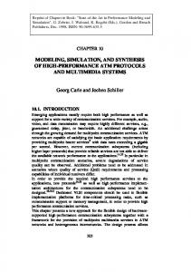
reconstruction of the yeast protein-protein interaction network, con�rmed experimentally, has demonstrated the existence of particular proteins that interact with many partners to connect di�erent biological processes ([48]). Another fact is that concepts needed for understanding biological systems, such as translation, inhibition or adaptation, arise from interactions among components ([22]). Another one is the robust functioning of modular models of biochemical networks ([65],[66]), that seems to be related to structural stability. In a higher biological level such as physiology, the modular approach has been useful to simulate human answers to changes of pressure or other stimuli, and to develop medicines to control these responses ([45], [46], [106], Figure 1.1). The detection of modules many times is non-trivial. To represent a system with interacting modules we must decide what elements act in coordinate way to group them, that is to say we must de�ne modules ([49, 88]). Essentially a module is a entity whose function is separable from those of other modules. To build modules we need to identify the functions, the elements that participate in them and how the interactions with other functions work. There are many factors to consider, such as the existence of hierarchy levels, speci�c and general functions, and the capacity of decomposing higher-level properties of the system into properties of modules. It is in the construction of modular models of biological systems that synthetic sciences, Mathematics, Computer Science and Engineering, play a fundamental role together with strong interactions with experimental and theoretical biology. There exists a relative consensus about considering hierarchical de�nitions of modules. In a hierarchical model there are de�ned several levels of complexity, the modules are de�ned by groups of variables and parameters in one level that are lumped together to form the elements of the high level of complexity. Consequently, a hierarchical
16
tel-00635273, version 1 - 24 Oct 2011
1.2. Composition and Hierarchy challenges
Figure 1.1: Guyton model [46]. The system is composed by 18 interconnected modules, each one modeling a di�erent function associated with the human circulatory physiology. Systems of di�erential equations, DAEs and other models are used in each module.
models could include the levels: molecule-cell-tissue-organ-organism-population of a biological system. There exists a set of tools have been used in di�erent cases to implement the notion of
module.
They can built, among many methodologies, by analyzing the
input-output responses of the interaction graph of the system, or grouping together nodes whose variations have comparable timescales ([49, 88]). Clustering tools have been used in some studies. In protein-protein interaction networks modules are de�ned by statistically analyzing topological properties like connectivity and the e�ect of remove proteins of the network. It is studied
in vivo
in silico in the modeled network, and
with knockouts of genes ([89, 48]). With the mathematical notion of modu-
larity, one quanti�es the quality of a division of a network by assigning high values to those in which there are dense connections between the nodes within modules but only sparse connections between di�erent modules ([52, 114]). To study the quality of the modular separation one can analyze if global model properties are inherited from the modules. ([88]).
One would want to ensure properties
stability and robustness of the model by these Sti�ness and timescales must be considered too.
such as
properties in its modules
17
Chapter 1. Introduction
1.2.2 Sti�ness and timescales Sti�ness is a property of mathematical equations. It is associated to the capacity of numerically solving a problem. It is mainly studied in di�erential equations, where one uses numerical integrators with discrete time steps. Sti�ness. A equation is sti� if numerical methods for solving it must use small time intervals to be accurate.
De�nition 1.8
Given a system, it is logical to have equations with di�erent sti�ness levels. Moreover, the interaction between processes developed in di�erent timescales produces a problem to solve complex systems.
Sometimes, to see the changes in
the behavior it is necessary to compare nearby times, but other times the changes happen in distant times. Often it is necessary to connect biological functions that pass in short time intervals with more slow functions. Both characteristics, di�erent
sti�ness
levels and
timescales, generate a compli-
tel-00635273, version 1 - 24 Oct 2011
cation to solve systems. Computation times and accuracy are a�ected. The use of modules solves in part these problems. If the equations solved by a module are sti� one uses smaller time intervals only at that module. If each module is capable to have its own timescale, one improves the representation of the processes of a system. In fact, sti�ness and timescales can be used as criteria to build or to qualify modules.
Ideally functions at the same module must have similar sti�ness and
timescales.
1.2.3 Composition: its challenges The act of building a model that is valid for two or more modules is called
sition.
Compo-
Let us consider the modules M1 and M2 (with two associated models). The composition of M1 and M2 is the model that explain the behavior of both interacting modules. De�nition 1.9
Composition.
An important need to develop science is to be able of reuse it. The advance of science is based on the reuse, the application and the improvements of the scienti�c discoveries. As said Isaac Newton, �... If I have seen a little further it is by standing on the shoulders of Giants.�
In the case of building models, we need reuse the
existing models to look beyond. A good implementation of this concept is essential to take advantage of the modularity of biological systems to build accurate and complete models. The de�nition of composition must be su�ciently �exible to be capable of joining modules de�ned with di�erent types of models, and to reuse modules that have been
a-priori
de-
�ned. This allows us to learn and to integrate knowledge of diverse type. The model can be extended and improved by introducing new modules that relates di�erent functions, or that model behaviors of factors. Another characteristic that one wishes is the reduction of composed system properties in properties of modules. That is to say, questions about the global system
18
1.3. Presence of randomness and use of Hybrid Systems in Biology must can be answered by analyzing the modules and the interaction between them. Ideally by looking the modules it must be easier to answer to functional questions. According to the observed relation between modularity and Hierarchy, the composition must be capable of including hierarchical relations to recover the
of
be part
relation. It must be possible to go up and down the levels by using reduction
operations that lump together variables and parameters and speci�cation operations respectively. The composition must answer coherently to re�nements of its modules.
If a
module is re�ned by adding information of its behavior, the composition of this module with another module must result re�ned. In the opposite direction one want to check re�nements of composed models by proving re�nements between modules, this is called
Assume-guarantee
rules of composition under re�nements.
It is necessary to impose technical requirements to avoid implementation problems. As explained in section 1.2.2, composition has to be capable of integrating
tel-00635273, version 1 - 24 Oct 2011
modules with di�erent sti�ness and timescales.
1.3 Presence of randomness and use of Hybrid Systems in Biology Randomness has two reasons to be present in biological models: sampling and incomplete information ([112]). Models are built by using data samples that allows us to build and validate them on a fraction of the total population. As we explained in section 1.1.1 one tries to use representative experimental data to obtain a good representation of the reality, but this statistical sampling always provokes the so called
sampling error
of the model.
The other important error source is the fact that the available information often is incomplete. Due to obtain biological data often is expensive, one needs to work with incomplete information. Moreover, the intrinsic unknown nature of some biological process makes di�cult to predict accurately the behavior. Non-deterministic and stochastic models allow us to include random decisions. These facts give space to randomness in Biology. One uses non-deterministic and stochastic models to include estimations of error and random (or non-deterministic) decisions. In addition, one considers Hybrid systems to combine di�erent types of factor a�ecting a biological system. One uses continuous models to describe gradual changes over time, discrete models for instantaneous changes, deterministic models to represent completely predictable behaviors and stochastic models to introduce randomness.
Changes in the conditions of the system, such as levels of nutrients
or environmental conditions can change the behavior laws (equations) of the system, or biological facts such as a gene is activated, to be expressed as protein, by a transcription factor or regulator give power to this approach. Hybrid systems as we de�ne them here (section 2.1), are one way to perform this combination. Some applications in biology are shown in [1]. In a recent article by Al�eri
et al
([3]) is used the theory of Hybrid systems to simulate the
R−point 19
Chapter 1. Introduction transitions that occur during the cell cycle.
Applications of Biotechnology to in-
dustrial processes, such as wine fermentation, are capable of approaching by Hybrid systems too (section 5). An important application area is
Gene Regulatory Networks
(section 6.2). Some
biological facts such as a gene is activated, to be expressed as protein, by a transcription factor or regulator give power to the idea of using
hybrid models.
In
this thesis (section 6), they are analyzed some hybrid models of Gene Regulatory Networks with applications in Cell di�erentiation ([36, 96]) and cell division cycle ([83, 40]).Another application area here considered was the modeling of wine fermentation kinetics by reconciling di�erent models ([10], section 5).
According to
initial condition levels and temporal phase the system switches between di�erent modes, to obtain good predictions of its dynamics.
tel-00635273, version 1 - 24 Oct 2011
1.4 Outline of this thesis In Chapter 2 we begin by describing the known elements about hybrid systems, and the particular case of switched systems in which the continuous dynamics is described by di�erential equations.
We continue by summarizing the theory of
stochastic transition systems, in which the discrete dynamics depend on stochastic decisions and schedulers that solve non-determinism.
Finally we explain the
main ideas about composition of models: synchronization of events according to the theory of transition systems and input-output connections. In Chapter 3 we present our modeling approach of complex biological systems. We begin by describing our approach to reuse and reconcile models. We recall the main arguments to use modular descriptions of biological systems (explained in this chapter), and present ideas about how to modeling biological systems by hybrid systems and composition. After that, we formalize the notion of hybrid system: the discrete dynamics of mode variables is described by stochastic transition systems, while the e�ect of the mode transitions on the continuous dynamics is described by coe�cient switches that modify coe�cients of the continuous model, or by strong switches that change the model itself.
We �nish by presenting the guarantees of
our approach, and summarizing the main contributions of this work with respect to modeling. In Chapter 4 we present the implementation of our modeling ideas and theories.
In the �rst section we describe the requirements of such a implementation.
After that, we describe the computation steps of the solving process, as a general schema independent of the implementation used. The next sections are related with the BioRica framework, which we use for implementing our approach. We explicit the contributions done in this thesis to the development of BioRica to satisfy the implementation requirements, and describe the implementation of hybrid systems with BioRica, the syntax, the semantics and the process of simulation. We �nish by summarizing the conclusions of this chapter. In Chapter 5 we apply the approach presented here to modeling, implementing and simulating the wine fermentation kinetics.
We analyze this application as a
particular case of reconciliation of competing models.
20
This hybrid model results
1.4. Outline of this thesis from the reconciliation of three wine fermentation models ([10]): Coleman ([28]), Scaglia ([94]) and Pizarro ([85], [92]). For each factor con�guration, one chooses the model that best �ts the experimental data of three papers: [85], [75] and [79] used as training. In function of the initial conditions one chooses the model and arriving at the stable fermentation phase, the model is updated to obtain the best predictions. The e�ect that produces the level of nutrients on the behavior of the system is successfully described by switching the model to include competence coe�cients when the resources are scarce. In Chapter 6 we apply our approach to cell fate decisions associated with the formation of speci�c cells. We describe these types of processes by using the theory of switched systems, reusing and composition of models. The di�erentiation process is described by a system of di�erential equations, wich is a�ected by regulatory processes (implemented by reusing SBML models) that switch coe�cients to favor one or other lineage. We focus in the case of bone and fat formation, in which the
tel-00635273, version 1 - 24 Oct 2011
dynamics of the di�erentiation of progenitor cells into osteoblasts and adipocytes is controlled by the interactions between di�erent processes. With this model, we want to predict the changes in bone or fat formation by stimulating (or inhibiting) the Wnt signaling pathway, the
P P ARγ
pathway, the division of progenitor cells,
and the apoptosis of progenitor or osteoblast cells. Based on this, one can analyze
in silico
the physiological responses to treatments of bone mass disorders based on
the Wnt signaling pathway, and to explore the e�ciency of new medical strategies before testing them in animal models. Finally in Chapter 7 we concludes and discusses the basis, scopes and future improvements of our work.
21
22
tel-00635273, version 1 - 24 Oct 2011
Chapter 2 Preliminaries Hybrid systems allow us to describe biological systems by including deterministic,
tel-00635273, version 1 - 24 Oct 2011
non-deterministic, stochastic, continuous and discrete elements. With this approach one captures behavior changes by using the theory of There are many applications of
Stochastic transition systems.
Hybrid models in other science areas.
In modeling
of physical phenomena it is usual to have partial or ordinary di�erential equations with right hands piecewise de�ned. Some classic examples are
heat and wave
tions, where changes in the medium produce hybrid systems ([95, 11]). models are very useful to analyze
electronic circuits
and
equa-
Hybrid
electrical networks.
Vari-
ables like the current are continues, while switches are real electronic dispositives ([58, 67]). In Biology, many dynamical systems are represented by ordinary di�erential equations.
Changes in environmental conditions or controlled factors modify the
development of diverse processes, which interact to realize the complex system behavior. In biological modeling randomness and non-determinism are common (section 1.3). The non-ambiguous combination of di�erent models by composition allows us to build complete models. One can reuse and reconcile existing models to obtain more general models.
2.1 Hybrid Systems According to our de�nition of
Complex Biological Systems
(de�nition 1.1), the com-
plexity of biological processes arises not only from the association of many components, but from the components too ([64]). One associates components with di�erent characteristics, properties and laws. This association of diverse behaviors carries to the use of represent biological processes.
Hybrid models
to
With the aim of obtaining good modeling, wide
range of models are allowed. The existence of di�erent types of models to explain connected processes makes to be necessary to de�ne tools to integrate them. Hybrid systems and models. One talks of Hybrid System if it responses to both continuous and discrete factors. Models that include both types of variables are called to be Hybrid models.
De�nition 2.1
23
Chapter 2. Preliminaries In our case, we are interested in
Hybrid dynamic systems.
They are described
using a mixture of continuous dynamics, discrete dynamics, and logical relations. n The dependent variables of the system, x = (x1 , . . . , xn ) ∈ R , are called
state vari-
ables
in analogy with Transition Systems. One considers as factors the continuous k variables u = (u1 , . . . , uk ) ∈ R , and the mode variables mode ∈ M = {1, . . . , M }. The values over time of these variables are called respectively the continuous and discrete dynamics. Hybrid Systems can be seen from two points of view: function ([18, 100, 104]) and implementation ([50, 60]).
The �rst one, called
switched systems,
focuses in
human comprehension, the second type is more general and focuses in automatic interpretation. This second approach uses tools of Automata theory and is easy to understand in terms of Transition Systems theory ([7, 29]). Continuous variables evolve according to continuous models, but at any time mode changes can change the de�nition of the continuous model. These changes are called
mode transitions
and are considered to be transitions in the sense of Transition Systems theory.
tel-00635273, version 1 - 24 Oct 2011
Given an action producing a mode transition, the next mode is chosen according to transition probabilities and system schedule laws. mode transitions are called
guards.
of its continuous dynamics.
The conditions that allow
For each mode, the system evolves in function
In literature, the discrete dynamics is modeled by
deterministic models, and allowing non-determinism with ambiguous guards. Here we extend the formal notion of hybrid system to include stochastic behaviors by considering stochastic transition systems ([29], section 2.2). Hybrid systems are described using a mixture of continuous, discrete dynamics and logical relations. The continuous and discrete dynamics interact, so that the changes in discrete variables provoke changes in continuous models and vice versa. To de�ne the dynamics of Hybrid Systems it is necessary to also describe interaction between the continuous and discrete dynamics.
2.1.1 Continuous dynamics The best known form of dynamic system is a set of ordinary di�erential equations. In such models, the dynamics of one or more variables (x) is described in a equation with the form shown in equation 2.1, where the temporal rates of are denoted
x(t) ˙
and called
temporal derivatives.
So, at any time
t
x
at time
t
the temporal
xi depends on a function (Fi ) of all the values of state x(t) and the values of continuous control variables u(t). One �nds notable
derivative of each variable variables
examples in classic mechanics such as the equation of motion, and in biological systems such as models of two or more populations competing by resources (LotkaVolterra equations, [98]).
x(t) ˙ = F (x(t), u(t)) The solution of equation 2.1 depends on the initial values of
ditions.
(2.1)
x,
called
initial con-
Often it is not possible to obtain solutions with explicit formulas, and one
has to use numerical methods to approximate the solutions at a given time using iterative schemes.
24
2.1. Hybrid Systems In addition, when physical or mechanical systems are determined by conservation laws, such as the conservation of energy or momentum, these systems are modeled by equation 2.2. variables
The function
G
is given by algebraic combinations of the state
x, derivatives x˙ and continuous control u, which is constrained to be equal
to zero. The model is called di�erential algebraic equations (DAE) ([38]).
G(x(t), ˙ x(t), u(t)) = 0
(2.2)
In general DAEs, we can use the form of equation 2.2 to separate the model into a system of di�erential equations and a set of implicit algebraic constraints (equations 2.3, 2.4). This is done by decomposing the variable ([68]). The vector of variables
x
x
into two variables
x
and
z
represents the dependent variables whose deriva-
tives are as in the equation 2.1, while
z
corresponds to algebraic variables whose
tel-00635273, version 1 - 24 Oct 2011
derivatives are not considered.
x(t) ˙ = H(x(t), u(t), z(t)) ˜ G(x(t), u(t), z(t)) = 0
(2.3) (2.4)
As example, let us consider the Lotka-Volterra equations ([98]) to model two populations: prey
x,
and predator
y.
If we assume that the prey have an unlim-
ited food supply (unlimited proliferation in absence of predator), the dynamics is described by the set of di�erential equations 2.5-2.6 below:
x(t) ˙ = x · (α − β · y) y(t) ˙ = −y · (γ − δ · x), where α
is the growth rate coe�cient of the prey,
β
(2.5) (2.6)
the rate of depredation coe�cient,
the predator mortality or emigration coe�cient, and
δ
γ
is associated to the growth
of the predator population. All of these coe�cients are considered to be positive constant over time. One can describes the same system but with limited supply by the DAE system with di�erential equations 2.7, 2.8 and algebraic constraints (with form 2.4) 2.9, 2.10. The coe�cients
β , γ , δ , a, b
and
F
are positive constant; while
α
and
z
are
algebraic variables.
x(t) ˙ = x · (α − β · y) y(t) ˙ = −y · (γ − δ · x) α=k·z a·x+b·y+z =F
(2.7) (2.8) (2.9) (2.10)
The equations 2.9 and 2.10 describe how the growth rate coe�cient decreases if the rate of food consumption
a·x+b·y
is near the allowed rate
F.
Partial di�erential equations are also common in many areas of science and technology. Such models use the form of equation 2.2, but
k−order derivatives of ones xj (i, j ∈ {1, . . . , n}). on
each state variable
xi
G
is allowed to depend
with respect to any of the other
25
Chapter 2. Preliminaries
2.1.2 Discrete dynamics The discrete dynamics is given by the changes over time of the mode variables
mode.
Discrete dynamics can be deterministic, stochastic or non-deterministic. Approaches from the implementation point of view favor the use of all these possible behaviors.
2.1.3 Interactions between continuous and discrete dynamics The way in which continuous and discrete models interact is by switches, which control changes in the continuous model by modifying the values of coe�cients or changing the de�nition of the continuous model (F in case of ordinary di�erential equations as 2.1, and in equation 2.2).
G
for DAE or partial di�erential equations with form shown
The discrete dynamics of the system, modeling the temporal
evolution of the discrete variables, is determined by such switches.
In the same
tel-00635273, version 1 - 24 Oct 2011
way that discrete dynamics can be stochastic or non-deterministic, the values of the discrete factors can provoke switches in the system both stochastically and non-deterministically. That is to say, given a discrete factor value it switches the continuous model according to deterministic, stochastic or non-deterministic rules. At the same time, the values over time of the discrete factors depend on time, the previous values, and the values of the state variables. Speci�c values of time or state variables provoke the change in the value of the discrete factors.
2.1.4 Switched Systems Hybrid system are the so called Switched Systems ([18, 100]). consider a Hybrid System whose model has continuous variables x and
An special type of Let us
discrete variables
m.
Independent of
x,
the value of the right hand function
changes in function of the value of discrete variable
m.
F
If for each value element of
con�guration. We will say in these cases, that changes in discrete variables values carry switches between model con�gurations, the Hybrid system is called Switched System. Each model con�guration is called a mode, the set M corresponds to the set of
S
the model change its form, laws, its equations: its
modes. To be capable of simulating it, generally it is assumed that there are only �nite switches in �nite time. Switched Systems, associated to di�erential equations 2.1, have the form of the equation 2.11.
x(t) ˙ = Fm(t) (x(t), u(t)), where
Fm(t)
depends on the mode
m(t).
It is to say,
(2.11)
m
de�nes the mode dynamics
of the system (Figure 2.1). The dynamics of
m
can be represented by the equation 2.12
m(t) = G(x(t), u(t), m(t− )),where G : Rn × Rk × M −→ M
(x(0) = x0 , u(0) = u0 , m(0) = i ∈ M ) the continuous trajectory time according to x(t) ˙ = Fi (x(t), u(t)), at the �rst time tj > 0 where
Starting at evolves over
26
(2.12)
2.2. Stochastic Transition Systems ∃j ∈ M : (x(·), u(·)) ∈ G(·, ·, i)−1 (j) the process continues. Other approach to represent Equations (
DAEs ).
(x(tj ), u(tj ), j)
then the variables become
switched systems is by a set of Di�erential Algebraic
This implicit representation takes the form of Equation 2.13.
˜ r (t), ur (t), m(t)) 0 = G(x The variables of
m(t)
xr
and
and
ur
are reduced versions of
there is di�erent
DAE
x
(2.13) and
u.
For each possible value
representing the system dynamics.
The implicit
equation 2.13 de�nes the discrete dynamics. It has a solution for each
m(t).
The
equation 2.1 gives the continuous dynamics.
A) General switched model
tel-00635273, version 1 - 24 Oct 2011
.
.
x=F1(x,u)
x=F2(x,u)
...
.
x=F|M|(x,u)
B) Switched model: Motion of a car . . s=v v=f1(u,v)
. . s=v v=f2(u,v)
. . s=v v=f4(u,v)
. . s=v v=f3(u,v)
s: position v: velocity u: throttle angle g: gear (1,2,3, 4)
Figure 2.1: A) : The dynamics of a Switched System. The model moves between di�erent modes, nodes in the picture, de�ning its discrete dynamics. At each mode, the system changes its continuous dynamics. B) : The Switched System of the motion of a car. The continuous dynamics, represented by the evolution of the variables position s and velocity v , changes its laws according to the engaged gear. A very intuitive example of switched system is the
a manual gearbox ([100], Figure 2.1).
Motion of an automobile with
This system is characterized by two continuous
variables: velocity and position. The manner in which these variables responds to the throttle angle depends on the engaged gear. In each
mode
of the engaged gear
the dynamics evolve in some continuous speci�c way. The dynamics of this system is hybrid in its nature.
2.2 Stochastic Transition Systems STS ) to describe transitions in Introduced by De Alfaro ([29]), STS cover the need
We use the theory of Stochastic transition systems ( Hybrid systems (section 2.1).
of modeling dynamics of biological systems with inclusion of uncertainty and the presence of uncontrolled external factors. The implemented notions of Composition
27
Chapter 2. Preliminaries and Synchronization allow us to de�ne systems by composing interacting modules and synchronizing actions. The state of the system in a given time is represented by the value of its ob-
interface
servable (
and
external ) state variables.
The system evolves over time by
changing its state. The transitions between states are caused by actions and spent time. One studies the stochastic behaviors of the system over time, depending on the actions at each state and the transition chosen for each action.
STS
correspond to Continuous Time Markov Decision Process (
section 2.2.3) in that one uses
randomized schedulers
CTMDP ) ([15],
to solve non-determinism in
simulations. The concepts were extended to continuous domains by using probability measures on sub set of states and actions ([25]). Let us begin with the theory.
De�nition 2.2
Transition
(Q, Q0 , A, −→) verifying:
System.
A Transition System S ([7]) is a tuple
tel-00635273, version 1 - 24 Oct 2011
1. Q is a set (commonly �nite) of states. 2. Q0 ⊂ Q is the set of possible initial states. 3. A is a set of actions. 4. −→ ⊂
(Q × A × Q) is the set of transitions.
a One denotes q → − q 0 if (q, a, q 0 ) ∈−→. One de�nes the set of actions available at the a state q as A(q) = {a ∈ A : ∃q0 withq → − q 0 }.
De�nition 2.3
Executions and observable executions.
De�nition 2.4
Sets of executions.
De�nition 2.5
Traces.
An execution is a sequence
0 σ = q0 a0 q1 . . . qn an qn+1 , . . .. If ∀i > 0 (qi , ai , qi+1 ) ∈−→ one says that σ = q0 − → an q1 , . . . , qn −→ qn+1 , . . . is observable in S.
a
Exec, Exec∗ , Execw denote the set of execu-
tions, �nite executions ending with an state, and in�nite executions respectively. A−traces.
Sequences of states are called Q−traces, of actions
The �rst state of a execution is �nite, is
σ
is denoted
f irst(σ).
The last one, if the execution
last(σ).
In the example (Figure 2.2), the set of states is
Q = {q0 , q1 , q2 }, q0 is the (unique)
A = {s, a, e}, and (q0 , s, q0 ), (q0 , a, q1 ), (q1 , e, q0 ) and (q1 , e, q2 ). An q0 sq0 aq1 with �nite trace of actions sa.
initial state, the set of actions is
the transitions of the system
are
observable �nite execution is
If ones assigns probabilities to the transitions, it is called a
System
Stochastic Transition
([29]).
One says that S is an Stochastic Transition System if it is a transition system (de�nition 2.2) that ful�lls 5 and 6.
De�nition 2.6
Stochastic Transition System.
5. An execution of S is chosen to start at q ∈ Q0 with probability P0 (q). 28
2.2. Stochastic Transition Systems
s
Initial action
e
q0
q1
a
q2
e
tel-00635273, version 1 - 24 Oct 2011
Figure 2.2: Example of Transition system for cell division. Circles represent states, black arrows transitions. Transitions are labeled by actions, but di�erent transitions can have the same label to represent that an action may produce many responses. The initial action selects the initial state of the system, always begin at q0 . States: q0 , q1 , q2 , transitions: (q0 , s, q0 ), (q0 , a, q1 ), (q1 , e, q0 ) and (q1 , e, q2 ). Red arrows are inherent idle transitions that are added to the system to assure in�nite executions, and to de�ne composition.
6. Given q ∈ Q, a ∈ A, the probability to choose to continue the state r ∈ Q, verifying (q, a, r) ∈−→, is Pa (q, r). In the example 2.2, for the state
q0
and
q2
q1
we see that given the action
e,
two successors
are possible. If we add probabilities to each option we have an Stochastic
Transition System. It is not necessary to de�ne probabilities to start the execution because only
q0
was considered as initial state.
2.2.1 Randomness and non-determinism We saw that randomness is present in the de�nition of Stochastic Transition Systems (de�nition 2.6): given an state and an action there are two or more possible transitions to continue the execution (Figure 2.2, state
q1
and action
The non-determinism arises from the fact that given an state observable execution, many actions could be available. not probabilistically modeled
a priori
a
an �nite
By de�nition, this fact is
and hence, to simulate executions, one must
solve it. In the example of Figure 2.2, given the state or the action
e). q of
q0
it could select the action
with di�erent successors.
A way of solving the non-determinism is to introduce the concept of
s
Scheduler.
The Scheduler, [113], speci�es the criteria to choose actions. They can be deterministic or randomized, with memory or not. With these elements, a �rst de�nition of randomized scheduler is:
A (randomized) scheduler is a function D : Exec −→ Distr(A) verifying that ∀σ ∈ Exec∗ supp(D(σ)) = A(last(σ)).
De�nition 2.7
Randomized Scheduler.
∗
With the aim of having in�nite executions one add an implicit
idle
transition
(that stay in the state) to each state of the Stochastic Transition System. sequently, an
STS
produces a
Markov Decision Process
Con-
(de�nition 2.8) for each
non-determinism solution.
29
Chapter 2. Preliminaries
De�nition 2.8
Markov Decision Processes generated by Stochastic Transition Sys-
If for each q ∈ Q we impose that A(q), the set of actions available at q, is non-empty for all q ∈ Q, the triple Π = (Q, A, P ) (with P given by Pa (q, r) the probability of a transition from q to r when action a is selected) is called a Markov Decision Process (MDP).
tems.
Let us consider our example (Figure 2.2) and the scheduler that selects after the state
q0
the action
s with probability 0.5 and the action a with probability 0.5.
This
scheduler allows us to obtain executions of the system and it does not have memory: it is not important how one arrives to a scheduler
D
q0
to decide the next action. We say that
is memoryless if it can be written as function from
as in this case.
Q
to
Distr(Q),
A scheduler is deterministic if it returns a Dirac distribution for
any execution, that is to say after each execution it is assigned an unique action to continue (for example if in
q0
the scheduler always selects the actions
a).
With these elements one can simulates the Transition System, whose results
tel-00635273, version 1 - 24 Oct 2011
depends of the scheduler that is chosen. But, what does the dynamics of the system represent? between a
what do the states represent?
Transition System
and
We have not established the relation
Dynamic models.
2.2.2 Dynamics of system variables: Probabilistic modules In the original approach of
Transition Systems
values of variables. Given a Transition System
Q
([7]), one associates states with
S = (Q, Q0 , A, −→),
represents a valuation of the system variables.
each state in
With this interpretation, state
transitions are changes in system variables values.
De�nition 2.9
Typed state variables.
It is considered the set x
of typed state
variables to be a set of names of variables, each one of them with �nite domain.
Q
X , at each state q ∈ Q the value of each The set Q0 is written as {q ∈ Q : q satis�es Θ},
is the �nite set of interpretations of
x ∈ X can be obtained. Θ is an assertion over X . Consequently, actions correspond to changes in the
variable where
system variables. Let us consider the example of Figure 2.2, and the following interpretation of states:
Variables: N : number of cells, A : activity level, G : growth. States (valuations of variables): • q0 = {A = 0, N = 1, G ∈ [0, 1]}, • q1 = {A = 1, N = 1, G ∈ [0, 1]}, • q2 = {A = 1, N = 2, G ∈ [0, 1]}.
Given a system, some variables are modeled and others, representing factors with unknown behavior, are not controlled. 2.2), let us consider that the growth part of the model, but only private or internal).
30
N
Continuing with our example (Figure
G
is not controlled while
A
and
N
are
can be accessed by other Transition System (A is
These considerations are denoted
ext = {G}, intf = {N }
2.2. Stochastic Transition Systems priv = {A}.
intf and external ext variables form the set of observable variables, obs = {N, G} in our example, while private and interface variables form the set of controlled variables, cont = {A, N }.
and
The interface
So, we can consider the following
Interpretation of the actions:
• initial action : ∅ −→ {N := 1, A := 0}, • s : {G, N, A} −→ if (G · N < 0.5) • a : {G, N, A} −→ if (A = 0)
{N := N, A := A},
{N := N, A := 1},
• e : {G, N, A} −→ if (A = 1, N = 1) {N := N + 1, A := A} N, A := 0} each option with probability 0.5.
tel-00635273, version 1 - 24 Oct 2011
In our example, only the action
s
and
a
{N :=
e is strictly probabilistic. The action s includes a G, not controlled by the model, and at q0 both
dependence on the external variable actions
∨
could be possible. The action
initial action
selects the �rst state,
the �rst valuation of variables that in this case is not probabilistic. As the external variables are not controlled by the system, the scheduler that selects the next action cannot depend on private variables of the module.
In order to correctly de�ne
schedulers on composition of modules, the controlled variables are partitioned into
atoms
(de�nition 2.10) with associated read variables.
An Stochastic Transition
System, with these interpretations of states and actions is called a
module
Probabilistic
(de�nition 2.11).
A probabilistic atom N consists of a set read(N ) ⊆ X of read variables, ctr(N ) ⊆ X of controlled variables, init(N ) an initial action from ∅ to ctr(N ), and an update action upd(N ) from read(N ) to ctr(N ). De�nition 2.10
Probabilistic X-atom.
De�nition 2.11
Probabilistic module.
parts:
A probabilistic module P consists of two
variables X(P ) partitioned into: ext(P ) the external variables, intf (P ) the interface variables, and priv(P ) the private variables.
•
Declaration:
•
Body:
�nite set atoms(P ) of probabilistic X(P )-atoms such that:
1. intf (P ) ∪ priv(P ) =
S
a∈atoms(P )
ctr(a),
2. ∀a1 , a2 ∈ atoms(P ) : ctr(a1 ) ∩ ctr(a2 ) = ∅. In summary, for each module we need a scheduler to simulate the environment (the initial and updated values for the external variables), and a scheduler for each atom to chose the initial values and the dynamics of the variables controlled by that atom (more details in subsection 2.3.1).
31
Chapter 2. Preliminaries
2.2.3 Inclusion of Time: Continuous-Time Markov Decision Process Although with these elements one can study the dynamics of the system, an important element is not considered: the advance of time. To each transition one can associates a unity of time, but it is logical to think that not all the transitions use the same quantity of time. The usual way to include time is by considering
transition times
and to link the
probabilities of successors with the time ([29], [113]).
De�nition 2.12
Stochastic Transition System as Timed Probabilistic System.
tel-00635273, version 1 - 24 Oct 2011
If we add to the Markov Decision Process Π = (Q, A, P ), the set of possible initial states Q0 and a labeling time function time, where time(q, a) is a non-negative value representing the expected amount of time spent at q when action a ∈ A(q) is chosen, Π = (Q, A, P, Q0 , time) is a Timed Probabilistic System (TPS). According to [29], some transitions can be
immediate
and others
delayed.
The
�rst ones have priority and do not spend time, the last ones have associated strictly positive times of transition. To relate spent times with the probability of transitions
P,
one considers that
for each action the spent time of transitions has exponential distribution. That is to say, one includes as part of the model a three-dimensional rate matrix
De�nition 2.13
Rate matrix.
R.
Is a three-dimensional matrix that satis�es:
1 R : Q × A × Q −→ R+ . 2 Given an state q and an selected action a, the probability that any of the successors is reached within time t is 1 − e−R(q,a,Q)·t , where R(q, a, Q) =
X
R(q, a, r)
r∈Q
3 Given an state q and a chosen action a, the transition is selected according to competition between possibilities. That is to say, the probability to chose the R(q,a,r) . successor r is Pa (q, r) = R(q,a,Q) Continuous-Time Markov Decision Process (CTMDP ), object that has been strongly studied in Probabilities ([15]). In this case
Π = (Q, A, R, P0 )
is called a
Exponential distributions describe the time between events, in a process in which
Poisson
the events occur continuously and independently at a constant average rate (
process,
[112]).
Given an state and an action, the properties
2
and
3
are direct
consequences of supposing that the transition options are time independent and exponentially distributed.
32
2.2. Stochastic Transition Systems In our example, Figure 2.2, by adding the rate matrix
R
to the model we have
that
R(q1 , e, q0 ) R(q1 , e, q0 ) + R(q1 , e, q2 ) R(q1 , e, q2 ) Pe (q1 , q2 ) = R(q1 , e, q0 ) + R(q1 , e, q2 ) Pe (q1 , q0 ) =
According to property action
a
2
in de�nition 2.13, the
soujourn time
in
q∈Q
under an
is determined by a exponential distribution that includes all the probable
q1 and the action e the soujourn time has exponential distribution with rate R(q1 , e, q0 ) + R(q1 , e, q2 ). −((R(q1 ,e,q0 )+R(q1 ,e,q2 )))·t The probability to reach an successor within time t is 1 − e . transitions to leave
q
by the action
a.
In our example, for the state
tel-00635273, version 1 - 24 Oct 2011
2.2.4 Schedulers and Timed executions As we explained in section 2.2.1, the existing non-determinism in Transition Systems is solved by
randomized schedulers.
A randomized scheduler assigns probabilities to
the possible actions given a �nite execution. When these probabilities are chosen, one can completely simulate the dynamics of the system. The dynamic of the model includes the time, consequently one can add the transition times to the notion of execution of a
Stochastic Transition System.
A timed execution is a possibly in�nite sequence of states, actions and time values σ = q0 a0 t0 q1 , . . . , qn an tn qn+1 , . . .. The set of timed executions, �nite timed executions ending with an state, and in�nite timed executions are denoted Σ, Σ∗ , Σw respectively. Given a stochastic transition system one says that a timed execution is observable if it can be obtained with probability not 0 by simulating the system. De�nition 2.14
Timed executions.
In our example, let us consider exponential distributions for spent times as is shown in the Figure 2.3. In addition, let us consider a randomized scheduler determinism in ity (0.5).
q0
by selecting both the actions
a
and
e
D
that solves the non-
with the same probabil-
On other states, the scheduler answers with the unique possible action
1). This scheduler is memoryless, it depends only on the current T > 0, we will compute the probability to obtain the �nite execution q0 aq1 eq2 with a total spent time lower than T . It corresponds to obtaining P ({q0 at1 q1 et2 q2 : t1 + t2 6 T }), assuming the scheduler to be D. At computing:
(with probability state.
Given
P ({q0 at1 q1 et2 q2 : t1 + t2 6 T }) = D(q0 )(a)Pa (q0 , q1 )D(q0 aq1 )(e)Pe (q1 , q2 )P (t1 + t2 6 T ) Z T Z T −t1 1 · 2e−2t1 · 2e−2t2 dt2 dt1 = 0.5 · 1 · 1 · 1 + 1 t1 =0 t2 =0 � = 0.25· 1 − (1 + 2T )e−2T For example, if
T =1
the probability is
0.25 · (1 − 3e−2 ) ≈ 0.1485. 33
Chapter 2. Preliminaries
s(1)
Initial action
e (1) q0
q1
a (2)
q2
e (1)
tel-00635273, version 1 - 24 Oct 2011
Figure 2.3: Example of Stochastic transition system. The presence of randomness (two possible successors of q1 under the action e: q0 and q2 ) and the time advance are modeled by considering that spent time of transitions has exponential distribution. We show the rate values R at each arrow between parenthesis. The non-determinism, associated to have two or more actions possible at the same state (case of q0 ), can be solved by a randomized scheduler that assigns them probabilities.
2.2.5 Extensions of Stochastic Transition Systems To continue we explore some of the main existing extensions of Stochastic Transition Systems, that generalize the notion of scheduler and the states and actions domains. It is possible to extend the notion of scheduler to consider that the selection of actions depends not only on previous states and actions, but also on the transition times that have been used ([25, 113]). It corresponds to functions from �nite timed ∗ executions (Σ ) to probability measures on actions (Distr(A))
A randomized timed history-dependent scheduler is a function D : Σ −→ Distr(A) verifying that ∀σ ∈ Σ∗ supp(D(σ)) = A(last(σ)).
De�nition 2.15
Randomized timed history-dependent scheduler. ∗
In the Figure 2.4, we show part of a transition system. To go out from are two possible actions:
a
and
b.
Let us consider the scheduler
� D2 (q0 ctq1 ) = where
δb
δa
b.
q1 ,
there
such that:
δa if t ∈ V δb otherwise,
is the distribution that selects the action
for the action
D2
a with probability 1, analogously
This scheduler satis�es the last de�nition, depending explicitly
on time. Thus, given this scheduler the probability to reach
Z
2e−2t dt
P (t ∈ V ) · Pa (q1 , q3 ) = t∈V that is de�ned if the set
V
is measurable in
q3
R+ .
in two steps is
·
1 , 2
Consequently, to include time
dependencies in the scheduler de�nition is necessary to have considerations on measurability. Another extension of scheduler arises from observing that an important element of non-determinism is not being considered: given an action, maybe one does not
34
2.2. Stochastic Transition Systems
Initial action
q0
q1
c (2)
b ( 2) a (1) a(
1)
q2 q3 q4
Figure 2.4: Stochastic Transition system with inclusion of rate values for spent times (between parenthesis). At state q1 two actions, a or b.
tel-00635273, version 1 - 24 Oct 2011
know the probability of each transition.
In our example (Figure 2.2), given the
e after q1 the probability to obtain each successor (q0 or q2 in this case) could be unknown (Pe (q1 , q0 ) and Pe (q1 , q2 ) with Stochastic Transition Systems notation, or R and if we work with exponential distributions of transition times). We need a
action
de�nition of scheduler that considers this case too. In [25] is introduced a wider de�nition of
Stochastic Transition System
that cor-
rects this last problem in the scheduler de�nition together with extending stochastic transition systems to continuous spaces of states and actions. Here, we modi�ed the de�nitions to allow a measurable set of possible initial states.
De�nition 2.16
Stochastic Transition Systems with continuous spaces.
tic Transition System is a tuple (Q, FQ ), Q0 , (A, FA ), −→ where: �
A Stochas-
• (Q, FQ ) is the analytic space of states, • Q0 ∈ FQ is the set of possible initial states, • (A, FA ) is the the analytic space of actions, • −→⊂ T = Q × A × Dist(Q, FQ ) is the set of probabilistic transitions. The fact that in a general model variables can take a continuity of values gives sense to allowing continuous states domains. The possibility of having continuous action spaces links the time to the associated action. It allows us to have models with general temporal distributions of transition times. But, as a consequence of this extension, the computations become more di�cult. The main analysis di�erence is the way to measure probability of executions, which appears the notion of
measure space of transitions and the scheduler de�nition
is adapted to the continuous case. Measure space of transitions. Given the set T = Q × A × Dist(Q, FQ ), it is de�ned the σ−algebra FT = FQ ⊗ FA ⊗ FDist(Q,FQ ) . Thus, (T, FT )
De�nition 2.17
is a measure space.
35
Chapter 2. Preliminaries FT
is the
set of measurable transitions.
It is formed by the product of measurable
sets of states, actions and probability measures that characterize the transitions. The set of
transitions enabled from a state q
Initial action
q0
q1
a
is
T (q) = {(r, a, µ) ∈−→ withr = q}.
e0
q*
e1
q2
e1
tel-00635273, version 1 - 24 Oct 2011
Figure 2.5: Stochastic Transition system with continuous space of states. The action e of our old example (Figure 2.2) was decomposed into two actions e0 and e1 . The action e0 has an in�nity of possible transitions: any q ∗ ∈ {{A = 1, N = 1, G ∈ [0, 1]} with G given byµ}. In Figure 2.5 we show a new stochastic transition system, in this example the action
e
of our old example (Figure 2.2) is decomposed into two actions
e0
and
e1 .
Let us consider that the states have the following interpretations:
� • q0 = A = 0, N = 1, G ∈ [0, 1] � • q1 = A = 1, N = 1, G ∈ [0, 1] � • q ∗ ∈ {A = 1, N = 1, G ∈ [0, 1]}, � • q2 = A = 1, N = 2, G ∈ [0, 1] So, the values of
G
with G given by the measure
are chosen by the probability measure
µ.
µ
We have that
Z P (q2 |q1 ) =
P (q2 |G)µ(dG) [0,1]
Let suppose that the action of
e1 has the following behavior (with V
a known subset
[0, 1]): ∗
� P q2 | q = {A = 1, N = 1, G ∈ [0, 1]} = P (q2 |q1 ) =
�
1 0
if
G∈V
otherwise,
R
µ(dG) = µ(V ), and we need V measurable in [0, 1]. V As in discrete case, the way to solve non-determinism is by using the scheduler
With this,
notion (de�nition 2.18). Given a �nite execution (where the time can be included in selected actions), it returns a probability measure over the set of probabilistic transitions
T
enabled from the last visited state.
De�nition 2.18
Scheduler (for STSs with continuous spaces). ∗
Dist(T, FT ) such that ∀σ ∈ Exec , supp(D(σ)) = T (last(σ)) 36
D : Exec∗ −→
2.2. Stochastic Transition Systems
2.2.6 Measurability of schedulers and executions In the previous section (2.2.5) we showed evidence for the need of including notions of measurability to analyze schedulers and executions. It is not possible to compute probabilities to any scheduler and execution. It is necessary to de�ne
schedulers, measurable probabilistic executions
measurable
and the relations between these ele-
ments. Although the discrete case of [113] can be seen as a sub case of the general stochastic transition systems of [25], for simplicity we will explain in detail the discrete approach. When one considers that schedulers can depend on previous transition times, it is necessary to impose measurability conditions to schedulers to be capable of computing probabilities of executions or timed executions (see section 2.2.5). With de�nition 2.19, the scheduler D2 in previous sub-section is measurable if and only + if V is measurable in R ( i� V ∈ Borel).
i.e.
tel-00635273, version 1 - 24 Oct 2011
De�nition 2.19
Measurability of timed history-dependent schedulers.
One will
say that a timed history-dependent scheduler is measurable if ∀L ∈ FA , D(·, L) : Exec∗ −→ [0, 1] (where D(·, L) is de�ned by D(σ, L) = D(σ)(L)) is a measurable function. To de�ne measurability of timed executions, one starts by de�ning the measurable sets of a given �nite length, the measurable sets of any length and �nally one joins the sets (de�nition 2.20).
De�nition 2.20
Measurability on sets of timed executions.
• As Q and A are considered to be �nite, for them one uses the powerset σ− algebras. To measure the time it is considered the Borel σ−algebra. • Thus, for the timed executions with length n, one generates FΣn = FQ×(A×R+ ×Q)n with the rectangles Q0 × M1 × . . . × Mn , where Q0 ∈ FQ , Mi ∈ FA×R+ ×Q . • The generators of FΣw are the cylinders with base a measurable rectangle in Σk , with k ∈ N. It is to say, it is generated by the sets R(Λ) = {σ ∈ Σw : σk ∈ R} where R is a rectangle in FΣk and σk is the pre�x of length k of σ. • Finally, for the arbitrary timed executions it is used the standard σ−algebra (FΣ ) formed by the disjoint union of the families {FΣn }n∈N and FΣw . In the case of
Stochastic Transition Systems with continuous spaces
([25]), the
notion of measurability of executions is similar, but measurability of schedulers is a little more di�cult to understand (de�nition 2.21).
De�nition 2.21
Measurability on set of executions with continuous spaces of states
and actions.
• As Q and A are considered to be continuous, one considers Λ = Q0 × A1 × Q1 × . . . × An × Qn the sequences of measurable sets (Qi ∈ FQ , Aj ∈ FA with i ∈ {0, . . . , n}, j ∈ {1, . . . , n}). 37
Chapter 2. Preliminaries • The set of �nite executions FExec∗ is the σ−algebra generated by all the the sets Λ, with n ∈ N. • Thus, the cylinders with base Λ are de�ned as CΛ = {q0 a1 q1 . . . an qn α} : ∀i ∈ {0, . . . , n}qi ∈ Qi , ∀i ∈ {1, . . . , n}ai ∈ Ai , α ∈ Exec • The set of measurable set of executions FExec is the σ−algebra generated by CΛ . To clarify concepts, let us consider the example of Figure 2.5 (section 2.2.5) with ∗ the successor of q chosen by a scheduler D3 de�ned such that:
�
∗
D3 (. . . q ) =
tel-00635273, version 1 - 24 Oct 2011
where
V
is a subset of
[0, 1]
q∗ ∈ V
otherwise,
P (q2 |q1 ) =
R V
µ(dG) = µ(V ),
and we need
V
to be capable to compute it.
One de�nes measurability of
continuous spaces
if
Q.
For this scheduler, the probability measurable in
q2 q0
Scheduler for Stochastic Transition Systems with
to relate measurable executions with measurable schedulers, gen-
eralizing the example.
De�nition 2.22
Measurability of schedulers, �attening of a scheduler.
• Given a scheduler (for Stochastic Transition Systems with continuous spaces) D, and σ ∈ Exec∗ a �nite execution. The probability measure µD(σ) over ((A × Q), FA ⊗ FQ ) de�ned ∀A ∈ FA , X ∈ FQ by: Z µD(σ) (A × X) = 1A (a)µ(X)dD(σ), (q,a,µ)∈T
is called the �attening of D in σ. • A scheduler is measurable if its �attening is a measurable as function from (Exec∗ , FExec∗ ) to (Dist(A × Q), FDist(A×Q) ) The �attening corresponds to the combined transition probability of actions and states to continue the executions.
That is to say, it measures the probability of
(FA ⊗ FQ ) (actions and probabilities) after the execution D.
continuing with each set in
σ
and with the scheduler In our example,
µD3 (·)
is a measurable function if and only if
µ−1 D3 (·) (1V ({q2 })) = V Thus,
D3
is measurable.
is a measurable scheduler if and only if
V
is measurable.
To link measurable schedulers with measurable executions, one introduces the notion of
probabilistic execution
and its measurability.
De�nition 2.23 Probabilistic execution and measurability. 38
2.3. Composition of models • Given an stochastic transition system (with continuous spaces) S and D a scheduler. The probabilistic execution PS,D for S and D is the tuple (Exec∗ , FA×Q , µ), where µ : Exec∗ × FA×Q −→ [0, 1] such that for each σ ∈ Exec∗ µ(σ, ·) de�ned by µD(σ) is a probability measure over A × Q. • A probabilistic execution PS,D = (Exec∗ , FA×Q , µ) is measurable if µ(·, X) is a measurable function for each X ∈ FA×Q . Consequently, a probabilistic execution de�nes the transitions probabilities induced by a scheduler and a �nite execution. In this case, from the measurability de�nitions one obtains the following measurability relation:
Theorem 2.1 Given an stochastic transition system (with continuous spaces) S ,
tel-00635273, version 1 - 24 Oct 2011
and D a scheduler. D is measurable if an only if PS,D is measurable.
2.3 Composition of models The composition of modules is based on two elements: synchronization of events and input-output relations. The �rst element is associated with the stochastic transition system (section 2.2) that describes the transitions of the hybrid system. By synchronizing two events we associate probabilistic modules by imposing that the occurrence of an speci�c event in one module coincides with the occurrence of another event in the other one. Given two modules, we use input-output connections to impose that the output of one module is input of other one. So, updates of the output imply updates of the input.
2.3.1 Composition of probabilistic modules Let's return to the previous section 2.2. The presence of sources of non-determinism allows that Stochastic Transition Systems can grow by joining modules to obtain more complete interacting models.
As we shown in our example (Figure 2.2 and
2.2.2), actions can depend on external variables not controlled by the module (action
s,
variable
G).
The dynamics of external variables can be considered to be modeled
by another module. As example, we consider that the dynamics of the variable module
Q
G
is given by the
(Figure 2.6), whose actions are:
• initial action : ∅ −→ g0 = {G := 0} ∨ g1 = {G := 0.5} ∨ g2 = {G := 1} probabilities
with
1 , 3
• g : {G} −→ {G := G + 0.5}, The module
Q
controls the behavior of
We connect the modules
composition
P
and
Q,
G,
the growth of the cell.
modeling division, by using the notion of
(de�nition 2.24, [30]).
39
Chapter 2. Preliminaries
g0
g1
g
g
g2
Initial action
tel-00635273, version 1 - 24 Oct 2011
Figure 2.6: Stochastic transition system that represents the behavior of G (growth of cell). It is formed by the states: g0 , g1 and g2 . The initial action selects with the same probability any state, the action g relates the states. Composition. The composition of two stochastic transition systems P and Q, denoted P ||Q, is the stochastic transition system that models the probabilistic behavior of P and Q that interact synchronously.
De�nition 2.24
For
probabilistic modules
(where states are interpreted as valuations of variables
and actions as probabilistic changes of its values, see section 2.2.2), the composition has to be consistent with respect to the mutually visible variables. It is to say, in a execution of
P ||Q,
the interface variables of
P
that are external variables of
Q (and
vice verse) must agree to have unique values per each observable variable. The modules
can be composed
if they are consistent with respect to the types of
variables. These facts are summarized in the following a�rmations:
•
•
Two modules,
P
and
Q,
can be composed if:
1.
ext(P ) ∪ intf (P ) = ext(Q) ∪ int(Q),
2.
intf (P ) ∩ intf (Q) = ∅,
3.
priv(P ) ∩ V (Q) = ∅,
4.
priv(Q) ∩ V (P ) = ∅.
If they can be composed, then
P ||Q
is a module such that:
1.
ext(P ||Q) = (ext(P ) ∪ ext(Q)) \ intf (P ||Q),
2.
intf (P ||Q) = intf (P ) ∪ intf (Q),
3.
priv(P ||Q) = priv(P ) ∪ priv(Q),
4.
atoms(P ||Q) = atoms(P ) ∪ atoms(Q).
The way to represent the behavior of a system is by obtaining the values of its answers, but it is not possible to use only the notion of execution. As stochastic
40
2.3. Composition of models transition systems include randomness and non-determinism, the number of different executions can be in�nite.
To add the stochastic element to the behavior
characterization, one de�nes the notion of
De�nition 2.25
bundle
([30]).
Bundles and semantics of probabilistic modules.
• A bundle of length n is a probability distribution over Q−traces of length n. • It is de�ned the semantics of a module P , denoted [[P ]], as the set of bundles
associated to the module.
Each bundle records the outcome of a particular sequence of randomized choices (answers of randomized schedulers) made by the system.
The use of randomized
schedulers, that transform non determinism in randomness, makes possible this de�nition. One can add the interpretation of the states in the semantics de�nition (de�nition
tel-00635273, version 1 - 24 Oct 2011
2.26) by replacing
Q−traces
bundles are probability over
by V −traces (with V the set of typed variables), V −traces and they are called V −bundles.
thus
To de�ne correctly the composition of modules, one considers only the observable variables, then
[[P ]]
is a probabilistic
(extl(P ) ∪ intf (P )-language
([30]).
If two modules P and Q can be composed, the semantics of the composition is the intersection of the both semantics, it is to say De�nition 2.26
Semantics of composition of probabilistic modules.
[[P ||Q]] = [[P ]] ∩ [[Q]]
. With de�nition 2.27, the equality the composition as
[[P ||Q]] = [[P ]] ∩ [[Q]] = [[P ]] × [[Q]]
de�nes
(VP ∪ VQ )−language.
Given two typed set of variables, VP and VQ for the modules P and Q respectively. Two bundles bP and bQ , for P and Q respectively, can be multiplied if bP [VP ∩ VQ ] = bQ [VP ∩ VQ ] (i.e. the probabilities coincide for VP ∩ VQ −traces). The product of bP and bQ bundles of length n, bP × bQ , is a (VP ∪ VQ )−bundle
De�nition 2.27
of length
n
Product of bundles.
such that
∀(VP ∪ VQ )−trace t (bP × bQ )(t) =
of length n:
bP (t[VP ]) · bQ (t[VQ ]) bP (t[VP ∩ VQ ])
An extension of our model of cell division is obtained by considering the modules
P
and
Q
(Figure 2.7), to allow
K
divisions of the cell.
We de�ned the concept of composition of modules that allows us to join di�erent models. However, in that notion do not exist restrictions about what actions are compatible. If a transitions happens in a module any possible transition is allowed in the other one, but often actions of di�erent systems are associated. In our example, a cell must grow if it is not capable of dividing, consequently the action if the action
s occurs in P .
of Transition Systems
This fact is included by de�ning the
g in Q happens
Synchronized product
([6, 24], de�nition 2.28).
41
Chapter 2. Preliminaries
q1
a
e
q2
e
...
e a
e
q0,1
q0,2
s
s
... ...
g
g1
qk
e
a
e
Initial action
g0
qk-1
a
e
q0,k-1
q0,k
s
s
e: {G,N,A}-> N:=N+1 or A:=0 q0,i= {G,N=i,A=0}, i=1, ..., k qi= {G,N=i,A=1}
g
...
gk-1
g
gk
tel-00635273, version 1 - 24 Oct 2011
... Initial action
g: {G}-> G:=G+(1/k) gi={G=i}, i=1, ..., k
Figure 2.7: Two Transition systems that at composing them represents the cell division process as depending on a growth index. Extension of models of Figure 2.2 and 2.6. We do not show the idle transitions at each state.
De�nition 2.28 Synchronized product of Transition Systems. Given n sets of actions A1 , . . . , An , and a synchronization constraint I ⊂ A1 × . . . × An . Let us T S1 , T S2 , . . . T Sn transition systems with states sets Qi , actions sets Ai , initial states Qi0 and transitions −→i for each i ∈ {1, . . . , n}. The synchronized product of � T S1 , . . . , T Sn is the transition system (Q1 × . . . Qn ), (Q10 × Qn0 ), (A1 , . . . , An ), −→ , de�ned by the following equivalence: (a1 ,...,an )
a
i → ri ) (q1 , . . . , qn ) −−−−−→ (r1 , . . . , rn ) ⇐⇒ (a1 , . . . , an ) ∈ I ∧ (∀1 6 i 6 n, qi −
With these composition elements one can build models formed by many interacting components. These ideas give the primary support to develop hierarchical models with di�erent complexity levels.
The inclusion of randomness and non-
determinism grants a major level of reality and �exibility to the models, to consider di�erent probable answers of the system and to improve models by composing them and synchronizing actions. The technical way to describe the concept of improvement of models is called
re�nement.
One wants that the re�nement relation behaves
well on compositions. That is to say, be capable of proving re�nement of composed models by checking re�nement properties on the components. This is achieved by having
assume-guarantee rules for composition under re�nements.
The de�nition of
composition of probabilistic modules satis�es a very strong rule. The re�nement of a probabilistic module intuitively corresponds to the speci�cation of the model. For example non-determinism reductions by associating probabil-
42
2.3. Composition of models ities to actions re�ne the module. A re�nement reduces the set of possible behaviors of the system. Re�nement of modules. One says that a probabilistic module P re�nes another module P ∗ if the following properties are satis�ed:
De�nition 2.29
1. intf (P ∗ ) ⊆ intf (P ), extl(P ∗ ) ⊆ extl(P ) ∪ intf (P ), 2. Given typed variables v1 , v2 ∈ intf (P ∗ ), if an atom A ∈ Atoms(P ) such that v1 , v2 ∈ ctr(A) then ∃A∗ ∈ Atoms(P ∗ ) such that v1 , v2 ∈ ctr(A∗ ), 3. ∀u ∈ intf (P ∗ ), v ∈ intf (P ∗ ) ∪ extl(P ∗ ), if ∃A ∈ Atoms(P ) : u ∈ ctr(A), v ∈ read(A) then ∃A∗ ∈ Atoms(P ∗ ) : u ∈ ctr(A∗ ), v ∈ read(A∗ ), 4. Bundle containment: [[P ]] is contained (⊆) in [[P ∗ ]]. tel-00635273, version 1 - 24 Oct 2011
The three �rst properties are structural, the last one relates the behaviors. It is clear that an stochastic transition system is a re�nement of a transition system. Solving non-determinism of a module by adding randomness schedulers to the module is a way to re�ne, as is adding composition or synchronization of two modules. One can prove ([30]) the validity of an circular
assume-guarantee
rule for
probabilistic modules given by the following assertion:
(P ||Q∗ � Q,
Q||P ∗ � Q∗ ) =⇒ P ||P ∗ � Q||Q∗
The utility of this rule is to prove that a composed module re�nes another when the module is composed by many components. Consequently, to check that the compo∗ ∗ sition of two modules Q||Q is re�ned by P ||P , it is su�cient to check re�nements ∗ of the components of the two original modules Q and Q . In particular, this says ∗ that to obtain a re�nement of Q||Q one must �nd a component P that, composed ∗ ∗ ∗ with Q , re�nes Q and other component P that composed with Q re�nes Q .
2.3.2 Input-output connections A natural way to integrate two models is by using the outputs of one as inputs of another one. It is useful to decompose extensive systems, or to connect processes
a priori
separated. In application sections (5 and 6), we will see how to use these
relations to build reconciled models (case of wine fermentation kinetics) and to connect regulatory systems to control cell fate. As example,
if we restrict the physiological circulatory model by Guyton
([45, 46, 106], Figure 1.1) to those modules of the renin-angiotensin-aldosterone system (RAAS) associated to renal control of the blood pressure (crucial for blood circulation [91]), we have the input-output connections in Figure 2.8.
43
tel-00635273, version 1 - 24 Oct 2011
Chapter 2. Preliminaries
Figure 2.8: Guyton model [46] restricted to the renin-angiotensin-aldosterone system. Systems of di�erential equations, DAEs and other models are used in each module, and they are connected by input-output relations. Rates variables: M DF LW (�uid in the renal tubules at macula densa), T V D (�uid intake), N OD, KOD, V U D (urine output), ADH (rate of hormone entry into the �uids). Concentrations: CKE , CN A, ADHC (antidiuretic hormone in the blood). Multiplier e�ects: AN M (angiotensin), AM K , AM N A, ADHM K .
44
Chapter 3
tel-00635273, version 1 - 24 Oct 2011
Our approach: Modeling biological systems Here we present our approach to describe complex biological systems by hybrid systems and composition of models, with the goal of modeling by reuse, reconciliation and composition of models. We formalize the theory of hybrid systems to combine continuous and discrete models, with the inclusion of stochastic and non-deterministic behaviors, and to allow two types of descriptions: with coe�cient switches and with strong switches (section 3.3).
The implementations of these descriptions with the new improved
version of the BioRica framework are presented in the next chapter (4). We �nish by summarizing the main contributions of this work.
3.1 Reusing and reconciling models by composition An important need to develop science is to be able to reuse it.
The advance of
science is based on the reuse, the application and the improvements of the scienti�c discoveries. In the last years research on reusability of models is vigorous ([109]), searching how to de�ne and simulate composed models in an unambiguous way is the goal we are approaching now. By accepting that biological systems are modular (section 1.2), the composition of di�erent modules allows us to build complete descriptions. Modularity allows us, between many things, to connect regulation and controlled models. Here, we compose models by connecting them by events synchronizations or input-output relations. Event synchronizations connect the discrete dynamics of the models, that is to say the stochastic transition systems. The composition of such systems, explained in section 2.3.1, allow us to combine di�erent discrete dynamics and to synchronize transitions. The input-output connections allow us to separate extensive continuous models into simpler models to solve them easier, or to combine the models of di�erent processes to describe more general behaviors. When a scienti�c area is attractive it is common that di�erent models are developed, each one constructed to meet particular needs and to �t speci�c data. We call
45
Chapter 3. Our approach: Modeling biological systems reconciliation of models the case in which di�erent models independently developed to describe a system, are analyzed to merge the best between them according to observable factors. The reconciliation process has three steps. In the �rst step we have the original models, which one can execute separately. In the second step, we can execute them in parallel using a single platform, and in the third we can control which model we use according to the factor conditions, for obtaining the best agreements to reality. For each system, we implement the last step of the reconciliation process in di�erent ways in function of the strength of the transformations induced by the switches. If it is possible to model those transformations as changes in the values of coe�cients, we rewrite all the possible models in a same base and identify common elements. In particular for ODE models, we rewrite the models into polynomial form. When the changes are stronger than changes in coe�cients, we use our approach with strong switches in the continuous dynamics.
tel-00635273, version 1 - 24 Oct 2011
First step: Independent models
Second step: Controlled models
Final step: A controller for homogenized equations
K Model 1
Model 2
...
K
Model N
Joining
Homogenizing Model 1
Model 2
...
Model N
Model 1... N
Figure 3.1: Reconciliation process. First we have the original models, then we control them to run them in parallel, �nally we control the selection of models to chose the best one in function of factor conditions. The diversity of models to explain connected processes makes it necessary to de�ne theory and tools to integrate them in a composed model. To compose models we use the non-ambiguous semantics of BioRica, which is based on the AltaRica framework ([7, 8]) and the use of Stochastic Transition Systems ([29]).
3.2 Modeling biological systems as Hybrid systems Due to the special conditions that one observes in biological systems: complexity of behaviors, dependence of environmental conditions, and modularity (section 1.3) we approach biological systems from the perspective of hybrid systems. We decompose the system into di�erent modules to represent individual processes. Each module is separately modeled, and we model the interactions between them by composition. In practice, the modeling process follows both directions. One starts by modeling individual biological processes, which can be modeled by decomposing into simpler modules and can be composed with other modules to describe more general processes. Each module is described by a model. Discrete controllers and controlled models de�ne Hybrid systems, and the composition of all these models is itself a hybrid system (section 3.4).
46
3.3. Describing hybrid systems DISCRETE MODEL x
Hybrid approach
DISCRETE MODEL x
mode
x
X MODEL
CONTINUOUS MODEL
Modeling
mode
Separating the continuous model
RESIDUAL MODEL
u
Input/Output Internal connections
tel-00635273, version 1 - 24 Oct 2011
Figure 3.2: Modeling schema of Complex Biological Systems using Hybrid models. First one identi�es the discrete and continuous interacting dynamics, then one separates the continuous dynamics into two interacting models: the X MODEL that describes the dynamics of X , and the residual model.
The possibility of composing models gives a way to improve and extend models, to obtain more and more complete descriptions of biological processes depending on the level of details that is wished and the quantity of available information. In absence of information, one can build models with open speci�cations by de�ning stochastic or non-determinist modules. This approach allows us to combine di�erent types of models to describe complex processes and to represent behavior changes provoked by environmental conditions. In particular, given a set of available models we can choose the `best' model according to the environmental conditions (section 5), and we can combine signaling pathways with Gene Regulatory Networks as in case of our model of cell fate decisions to form bone or not (section 6).
3.3 Describing hybrid systems As we explained before (section 2.1), Hybrid Systems can be seen from two points of view: function ([18, 100], [104]) and implementation ([50, 60]).
The �rst one,
called Switched Systems, focuses in human comprehension, the second type is more general and focuses in automatic interpretation. This second approach uses tools of Automata theory and is easy to understand in terms of Transition systems theory ([7, 29]). Our approach uses elements of both approaches. Most of continuous models are given by sets of ordinary di�erential equations, but we allow other type of continuous models, which can be speci�ed externally by using the SBML speci�cation ([56]). Continuous variables evolve according to continuous models, but at any time mode changes can change the de�nition of the continuous model. are called
mode transitions
These changes
and are considered to be transitions in the sense of
Transition Systems theory. Given an action producing a mode transition, the next mode is chosen according to transition probabilities and system schedule laws. The conditions that provoke mode transitions are called
guards.
For each mode, the
system evolves in function of its continuous dynamics.
47
Chapter 3. Our approach: Modeling biological systems Our use of Stochastic transition systems ([29]) to describe mode transitions, allows us to extend the notion of Hybrid system (section 2.1) to include stochastic and non-deterministic behaviors.
To model hybrid systems, we consider that the
continuous dynamics is given by ordinary di�erential equations or other models, while the discrete dynamics is described by Stochastic transition systems as de�ned in section 2.2 with general temporal distributions for mode transitions (not only exponential ones). Using modular representation is possible to include logic based functions to de�ne hybrid systems. Input/output connections, switches, control and hierarchical relations relate modules.
3.3.1 Formalization According to the theory of
stochastic transition systems (section 2.2), the transitions
may have stochastic and non-deterministic behaviors. Given an action producing a transition, in this case a mode change, the following mode is chosen randomly
tel-00635273, version 1 - 24 Oct 2011
according to transition probabilities. Formally, the model is represented as systems whose continuous model has transitions given by the following equations 3.1,3.2, and 3.3 above:
P (ev|(x(t), u(t), mode(t)) the probability of choosing the event ev when the values of the state variables x are x(t), the values of the continuous control variables u are u(t) and the value of the mode variable mode is mode(t); time((x(t), u(t), mode(t)), ev) denotes the delay time of the event ev that is modeled to have distribution Distev {pevent,1 , . . . , pevent,m }. At any time
t,
we denote
P (ev|(x(t), u(t), mode(t)) =
wev X
,
(3.1)
time((x(t), u(t), mode(t)), ev) ∼ Distev {pevent,1 , . . . , pevent,m },
(3.2)
we
e∈A(x(t),u(t),mode(t))
where is the mode
we is the probability weight assigned to the event e, and A(x(t), u(t), mode(t)) set of available actions when x takes the value x(t), u the values u(t) and the variable mode the value mode(t) (equation 3.3).
A(x(t), u(t), mode(t)) = {ev ∈ EV EN T S : Gev (x(t), u(t), mode(t)) = T RU E} (3.3) , and
EV EN T S
is the set of events considered.
3.3.2 Two types of hybrid systems: with coe�cient switches and with strong switches Systems are described here as Hybrid systems, whose modules are described by models. We consider two classes of switches: coe�cient switches and strong switches. We call Hybrid system with coe�cient switches those hybrid systems in which the structure of the model is conserved and only speci�c coe�cient values are controlled by the mode transitions. The continuous model is composed of an unique controlled model
X MODEL that interacts with the controller CONTROL (Figure 3.3(A) ). We
de�ne Hybrid systems with strong switches as hybrid systems that allow di�erent
48
3.3. Describing hybrid systems types of models. In such a case, each type of continuous model is represented by two interacting modules:
MODEL i
and
CON T ROLi
(Figure 3.3
(B) ).
In the case of Switched Systems, where one assumes continuous dynamics based on di�erential equations, the global dynamics comes from the interaction of the continuous and the discrete dynamics, a�ecting the di�erential equations.
Mode
transitions provoke changes in the continuous dynamics without changing the structure of the module, but only values of coe�cients (Figure 3.3
(A)
Discrete model
MODE u
x
off
(B)
on
mode
MODE 1 u
x
X MODEL (Controlled model)
tel-00635273, version 1 - 24 Oct 2011
Continuous model
u
off
on
...
MODE j
mode
Model 1
u
...
(A) ).
off
x
on
... MODE N
mode
u
x
...
Model j
off on
mode
Model N
x
CONTROL (Continuous Control)
CONTROL1
...
CONTROLj
...
CONTROLN
Figure 3.3: Abstraction of Hybrid systems. (A) The module X MODEL describes the continuous model of the state variables x. It interacts with two other modules: CON T ROL and M ODE . CON T ROL computes the values of the continuous control variables u, M ODE decides the values of the mode variables. Arrows denote input-output relations. (B) Strong switches between N models. The j−th model is represented by its continuous dynamics M odel j , that interacts with two modules: the controller CON T ROLj , and M ODE j that decides if the model is active or not. For strong switches, the system takes the form of Figure 3.3 modules
M ODE i,
(B). By means of the
the system switches between di�erent modules that represent
di�erent types of continuous models. At the same time, each module
M odel j
can
interact with its continuous controller and evolves over time. When each continuous dynamics has a di�erent type of formalism, software or type of mathematical description, the possible continuous models can not be uniquely represented considering switches as changes in its coe�cients. When one has access to all the models, considering the models as structurally di�erent or not is a modeling decision.
Let's suppose for example that we know
that given an speci�c condition a variable other variable
xj ,
xi
responses linearly with respect to
but in other condition this dependence is quadratic. One must
decide to join the models, by linear combination of both dependences and choosing the coe�cients in function of the conditions, or to consider them separately. If one decides to join di�erent models, to use Hybrid systems with coe�cient changes, one must rewrite the models to represent them within an unique structure by identifying types of dependences and by grouping them.
However, in general
cases rewriting is not the best option. The rewriting of models can help to interpret the results, but it consumes time, increases the possibility of mistakes, and it is not practical to have to rewrite models whenever we want to reuse them. Moreover, if one does not have access to one model but to the state variables values computed by it (e.g: executing a software), this option is not possible. Such a model is seen
49
Chapter 3. Our approach: Modeling biological systems as a black box with a di�erent structure, and the system is modeled with strong switches.
(B) )
If we consider the approach strong switches (Figure 3.3 mode modules in an unique module
M ODE
and group all the
and consider the control modules in-
cluded in each model, this corresponds to the case when many models are used to describe the same system and we reconcile the models into an unique one (Figure
M ODE
3.4): a reconciled model where module
considers the associated mode vari-
able active if the factor values belong to the optimal conditions, chosen according to the calibration of the model or validating on new data. From the de�nition of Hybrid systems (section 2.1), one observes that the system resulting from reconciling models is a Hybrid system.
mode 1: off
MODE
mode j: off
tel-00635273, version 1 - 24 Oct 2011
mode N: off
... .. .
on on on
X(N)
X(1) mode 1 ... Model 1
...
mode N mode j
X(j)
Model j
... ...
Model N
Figure 3.4: Abstraction of the reconciliation of models as hybrid system with strong switches. The j−th model is represented by its continuous dynamics M odel j , that interacts with two modules: the controller CON T ROLj , and M ODES that decides if the model is active or not by means of the mode variable mode j . With this approach it is possible to describe Hybrid systems with coe�cient switches and with strong switches within a single formalism. independent of the type of continuous dynamics.
This approach is
The modeler can chose which
models to join in an common module and which ones to consider as di�erent modules according to common characteristics and accessibility of the models.
3.4 Guarantees We obtain some assume-guarantee rules with respect to properties of Hybrid systems and compositions of them. The stability (in the sense of Lyapunov) of Switched systems is not direct from the stability of each model con�guration, one has to study the interactions between the continuous and discrete dynamics.
As a result, stability is assured given the
conditions of Theorem 6 in [18], which establishes the required properties of the so called switching sequences (initial states values and mode-time pairs of switches):
50
3.5. General contributions `existence of Lyapunov-like functions that satisfy the non increasing condition, and mode variables forming a compact set'. Other hybrid systems properties are presented in [50]. It de�nes decidability properties of veri�cation tasks such as reachability, emptiness and trace inclusion problems on hybrid systems or subsets of them. The theory presented here allows us to obtain two properties that are closed with respect to the composition of hybrid systems: the de�nition itself, and the re�nement of hybrid systems. From section 2.3 is clear that the composition of hybrid systems, by event synchronizations or input-output connections, is a hybrid system. Compositions of the associated stochastic transition systems are stochastic transition systems, and the result of joining continuous models by inputs/outputs connections is a continuous model. As we explained in section 2.3.1, the re�nement of a module forming part of a composed system results in a re�nement of the composed system. That is to say, if
tel-00635273, version 1 - 24 Oct 2011
one speci�es the behavior of one module by restricting its behavior (its model) as result one speci�es the composed model. So, the process of improving models can be carried out by improving the individual models of the composed system. Our approach assures the consistency of composed models with respect to the state variables. That is to say, given a composed model and a variable that is used by many sub-models, one can control how the changes on this variable are perceived by the sub-models. It is obtained by associating a �ow variable to each shared variable, and imposing assertions of equality between the versions of that �ow variable on di�erent modules.
3.5 General contributions In this chapter we have presented the development of an approach with theoretical substance and good results in practice.
It allows modeling, implementation and
simulation of real biological applications. Concrete examples will be seen in later chapters. This approach takes its place in themes of current research: composition and reusing of models, and coupling of metabolic pathways and Gene Regulatory Networks.
Composition of validated models is considered a way to build complete
descriptions of complex biological systems ([109, 33]). Our approach and the BioRica framework allow us to combine di�erent types of models, by implementing the notion of composition and importing SBML models. Metabolic coupling in Gene Regulatory Networks ([12]) has been considered as a way to obtain indirect interaction between genes, to obtain better descriptions of underlying behaviors. We further considered formalization of the Hybrid Systems theory by using Stochastic Transition Systems ([29]) to describe stochastic and non-deterministic changes of the continuous dynamics.
This allows us to include general temporal
distributions of mode transitions, which are responsible of model changes according to two possible types of transformations: coe�cient switches and strong switches. For coe�cient switches the structure of the model is conserved, and mode transitions provoke changes in their coe�cients. For strong switches, the system switches
51
Chapter 3. Our approach: Modeling biological systems between di�erent modules that represent di�erent types of continuous models. With this theory one can consider di�erent levels of model changes according to the modeling decisions, coe�cient switches are done by modifying the models, while with strong switches the models are directly reused. We obtain some assume-guarantee rules with respect to properties of Hybrid systems and compositions of them.
The stability (in the sense of Lyapunov) of
Switched systems is assured given the conditions of Theorem 6 in [18]. Compositions of Hybrid systems are Hybrid systems, and re�ning of a module forming part of a composed system results in a re�nement of the composed system. The consistency of composed models, with respect to shared variables, is assured too. More details in section 3.4. We have identi�ed implementation challenges: sti�ness, di�erent timescales, and transitions happening in not considered times; and we have proposed solutions: the current use of modules with independent solvers, and the future possibility of including solvers based on the QSS (Quantized States Systems, [68]) approach.
tel-00635273, version 1 - 24 Oct 2011
The development of the theoretical basis of our approach was complemented with the improving of the BioRica framework.
We identi�ed problems of the previous
BioRica version, and proposed solutions that contributed to the development of important improvements included in the current version with the aim of modeling real biological systems, composing models and allowing hybrid systems. More details can be seen in section 4.3.2.
52
Chapter 4
tel-00635273, version 1 - 24 Oct 2011
Our implementation: Simulating biological systems In the previous section (3), we explained how to describe complex biological systems by using hybrid systems. This theory allows us to describe interaction of di�erent processes, which are separately modeled by using di�erent types of dynamics. The inclusion of hierarchical relations, combination, reusing, and reconciliation of models gives the possibility of building complete descriptions of biological systems. Here we focus on the implementation of these ideas and theories, we go from the theory to the practice. To take advantage of all the qualities of the theory, the implementation must allows general de�nitions of hybrid systems, and reusing existing models. We need a framework able to solve systems with continuos, di�erential equations systems, and discrete interacting dynamics. We start by discussing the requirements of the implementation, and describing the di�erent steps to solve hybrid systems to obtain a general schema of the solution process.
After that, we argue our decision of implementing these steps with the
BioRica framework, which we contributed to improve and extend to work with hybrid systems.
4.1 Requirements of the implementation We describe the main requirements are necessary to implement our approach. Some needs are related with the way of solving and coding hybrid systems, others with the possibility of composing and reusing models.
1. Able to solve continuous models. In particular, we need to solve systems of di�erential equations with di�erent complexity degrees (sti�ness, section 1.2.2) and work with di�erent timescales. 2. Able to solve discrete models given by stochastic transition systems (2.2), which are used by our de�nition of hybrid systems. We require de�ne mode transitions with inclusion of stochastic and non-deterministic decisions, which are associated with the chosen transition, action and the spent time.
53
Chapter 4. Our implementation: Simulating biological systems 3. Previous points are related with the ability to solve a wide range of models. In addition, we must be able to use them in the same framework. The framework must be capable of integrating di�erent types of solvers, which are adapted to solve speci�c models, without being a compendium of di�erent programming languages.
4. Able to implement composition. The combination of di�erent types of models by means of input-output connections (assertions), event synchronizations is fundamental in our modeling approach.
5. Able to incorporate hierarchical relations between models.
It allows us to
de�ne control relations between processes, and to go from macroscopic to
tel-00635273, version 1 - 24 Oct 2011
microscopic descriptions levels.
6. Able to implement reusing of models. The framework must allow the reutilization of validated models without rewriting them.
4.2 Solving hybrid systems Here we describe the solving process of hybrid system. The process is independent of which framework is used to implement our approach. Figure 4.1 shows the computation steps to solve a hybrid system with state variables
x
and mode variables
IC
mode.
The process begins reading inputs: initial
P . The time is initialized to zero, and the initial values of the mode variables mode(0) are computed in function of the input values. Then the initial de�nition of the model M ODEL(mode(0)) is obtained. The conditions
and parameters values
next steps of the diagram are the main part of the process: solving and updating. At any given time the model is solved, and the model is updated when detecting
M guard conditions associated to each possible new value of mode (denoted by GU ARD(x, mode, u, time) in Figure 4.1). The process �nishes when EN D(x, mode, time) is veri�ed and the results are printed. one of the the
This general schema (Figure 4.1) allows both types of hybrid systems we de�ned in section 3. According to the e�ect of the assignation
M ODEL(mode) after updat-
ing a mode, we can be solving hybrid systems with coe�cient switches which just change coe�cient values, or with strong switches by changing of model in function of the value of
mode
(Figure 3.3). As we anticipated, to implement this solution
schema we used BioRica. As we explained in section 3, the type of hybrid system chosen is a modeling decision. Given a system, one uses coe�cient switches to conserve a basic structure of the model and using mode transitions to do changes in their coe�cients.
On
the other hand, for strong switches, one considers that the system switches between di�erent types of continuous models to allow the reusing of models. The combination of many models favor the use of the strong switches approach.
54
4.3. Improving the BioRica framework for simulating biological systems NO
(IC,P)=READ INPUTS
TIME= 0 mode (0 )= mode ( IC, P )
MODEL= MODEL (mode(0))
x= SOLVE (MODEL,TIME, IC, P) TIME= INCREMENT (TIME)
NO GUARD (x, mode, u, TIME)?
YES END (x, mode, u, TIME)?
PRINT
YES END
START
tel-00635273, version 1 - 24 Oct 2011
Update mode MODEL= MODEL (mode)
Figure 4.1: Computation steps to solve an hybrid system, options used for wine fermentation shown in red. The process begins reading inputs: initial conditions IC and parameters values P . It is initialized the time in 0, and computed the initial values of the mode variables. Then, one obtains the initial de�nition of the model M ODEL(mode(0)). At any time the model is solved, it is updated when detecting the guard condition GU ARD(x, mode, u, time), and the process �nishes when it is veri�ed EN D(x, mode, u, time).
4.3 Improving the BioRica framework for simulating biological systems The implementation of our ideas is based on the BioRica framework. The improved version of BioRica (section 4.4) satis�es the requirements of section 4.1. Modules are described by BioRica nodes, which interact to model the emergent properties of the system. The current version of BioRica was developed by Alice Garcia in the MAGNOME team and is distributed under an open source license. It allows one to describe hybrid systems, solving di�erential equations and simulating stochastic and non-deterministic behaviors, together with reusing and combining existing models.
4.3.1 The BioRica prototype The creation of BioRica was motivated by the idea of applying the ideas of AltaRica Data�ow language ([7, 8]) to biological systems. This �rst extension looks for describing stochastic transition systems (section 2.2, [29]) by incorporating stochastic and timed behaviors, and data�ow links to include composition. A prototype, used internally by the MAGNOME team was developed ([101]). Each BioRica node is composed by the speci�cation of its �elds: state, �ow,
state, one declares the state �ow, one includes inputs (or outputs) from (to) other BioRica nodes and the �eld sub de�nes other node objects the node use (hierarchy notion). In event one declares the names of the possible actions, and the transitions sub, event, trans, assert, init and extern. In the �eld
variables and their domains. In
provoked by these events (when they happen and the e�ects) are described within the key in
init
trans.
In
assert,
one imposes relations between �ows and/or states, and
one de�nes the initial values of the state variables. Finally, the �eld
extern
allows the inclusion of external directives about distributions of event delays and priority between events.
55
Chapter 4. Our implementation: Simulating biological systems BioRica de�nes a global semantics to compose interacting modules. It is based on the automata semantics of AltaRica ([7, 8]), and the theory of Stochastic Transition Systems ([29]) that allow the inclusion of randomness and non-determinism. Given a BioRica node, one computes the probability of the state dynamics and considers non-deterministic decisions solved by random schedulers. The simulation generates a trace giving the values of the system variables at each times. The resulting semantics it is preserved with respect to �ow relations and event synchronizations. Although they constituted the �rst theoretical ideas about BioRica as compositional tool for stochastic transition system (requirements
2, 4
and
5
of section 4.1),
the usability of this framework would require many improvements and extensions.
4.3.2 Improving BioRica During this work we have contributed to the development of the new implementation of BioRica by suggesting extensions, discussing implementations, and proveding ap-
tel-00635273, version 1 - 24 Oct 2011
plications. This version includes important improvements to be capable of modeling real biological systems. We detected the problems of the previous version, proposed and checked possible solutions. As result, with the new version we are capable of describing biological systems as hybrid systems that integrates continuous, discrete, deterministic, stochastic and non-deterministic behaviors. Here we present our main contributions.
•
Identi�cation of the need to recode and redesign the BioRica prototype, to build an uni�ed, structured and usable tool of mathematical modeling of biological systems. The implementation of the old version used many di�erent programming languages, and its applicability was limited to discrete models with integer variables.
•
Identi�cation and modeling of biological systems not implementable with the BioRica prototype.
For discrete systems, we established the need to de�ne
transition computations using not only the basic algebraic operations and integer variables. To describe more general systems it was necessary to include continuous elements, which carried to the use of hybrid systems.
•
A decision to abandon Matlab as external numerical tool to compute not basic algebraic operations and to solve di�erential equations. The bridge between the BioRica prototype and Matlab, by means of the engine library of
C + +,
worked too slowly and complicated signi�cantly the implementations.
•
A decision to adopt the Python libraries to compute general algebraic operations and to solve systems of di�erential equations, and the possibility to include new libraries to solve other types of equations. The new implementation of BioRica by using Python makes it easy to use all the Python libraries which are available free and have permanent development.
•
Modeling and BioRica speci�cation of Hybrid Systems by composing their continuous parts and discrete controllers, assuring integrity of individual models and including hierarchical relations.
56
4.4. Implementing and simulating hybrid systems with BioRica •
Development of an approach to reconciliate competing models based on Hybrid Systems theory. Modeling and BioRica speci�cation of that approach.
•
Development of a general modeling and BioRica implementation of Switched Systems, particular type of Hybrid System in which continuous models are systems of di�erential equations, by using two types of model changes: coe�cient switches and strong switches.
•
Proposition of a new BioRica syntax to allow descriptions of general hybrid systems with other continuous models or external implementations. By using other Python libraries one would solve hybrid systems in which the continuous model is described by models such as di�erential algebraic equations or partial
tel-00635273, version 1 - 24 Oct 2011
di�erential equations.
4.4 Implementing and simulating hybrid systems with BioRica We code and simulate the computations steps needed to solve hybrid systems (Figure 4.1) with BioRica. So, modules are implemented by BioRica nodes. The BioRica syntax is su�ciently general to describe these types of systems with many interacting components, the implementation here explained satis�es all the requirements of section 4.1. To de�ne BioRica nodes we use the structure of Figure 4.2 that implements the abstractions of Figure 3.3.
When mode transitions only change the values of
coe�cients of the continuous model, we use the approach of Figure 4.2(A). If the changes are stronger than simple changes in coe�cients values, we consider the approach of Figure 4.2(B) for strong switches. continuous model, while the nodes
M ODE i
Each node
M odel j
represents a
control if each model is active by
deciding the value of the mode variables associated.
In case of reconciliation of
models, the mode variables are grouped and each continuous model is represented by only one module. In Figure 4.2 we do not include all the possible �elds, such as temporal laws or synchronizations between events. Event synchronizations can be used to reduce the number of assignments in input-output connections, improving the computing time. So, for example for coe�cient switches, the node if mode transitions happen in the node
M ODE
X
updates the value of
mode
just
(Figure 4.2). In simple cases, the
discrete and continuous dynamics can be included in the same node (Figure 4.3). For see examples of extensive models go to application chapters (sections 5 and 6). The process can continue. This implementation approach allows the reuse of the combined models. So, the notion of compositions is implemented allowing combination, reusing and reconciling of models.
4.4.1 Syntax and semantics of BioRica for hybrid systems BioRica allows the interaction between continuous and discrete dynamics.
The
current version of BioRica considers continuous dynamics given by sets of ordinary
57
Chapter 4. Our implementation: Simulating biological systems (B)
(A) node MODE state _mode:{1,...,N}; flow x1,...,xn,,u1,...,uk:FLOAT:in; mode:{1,...,M}:out; event mode_transition; trans GUARD1(x1,...,xn,u1,...,uk,mode,time)|-mode_transition -> _mode=1; . . . GUARDN(x1,...,xn,u1,...,uk,mode,time)|-mode_transition -> _mode=M; assert
node MODEj state _mode:{0,1}; flow x1,...,xn,,u1,...,uk:FLOAT:in; mode:{0,1}:out; event mode_transition; trans on(x1,...,xn,u1,...,uk,modej,time)|-mode_transition -> _mode=1; off(x1,...,xn,u1,...,uk,modej,time)|-mode_transition -> _mode=0;
assert
mode=_mode;
mode=_mode;
init
init
_mode:=mode(0); law ... edon
_mode:=mode(0); law ... edon
Discrete model
MODE u
x
off
on
MODE 1 mode
X MODEL (Controlled model)
Continuous model
u
u
off
x
on
...
MODE j
mode
Model 1
x
u
off
x
on
mode
Model j
...
... MODE N u
off on
x
mode
Model N
...
CONTROL (Continuous Control) CONTROL1
...
CONTROLj
...
CONTROLN
node MAIN sub Mode:MODE; modelX:X;
tel-00635273, version 1 - 24 Oct 2011
Control:CONTROL; assert Mode.x1=modelX.x1;...;Mode.xn=modelX.xn; modelX.mode=Mode.mode; Mode.u1=Control.u1;...;Mode.uk=Control.uk; modelX.u1=Control.u1;...;modelX.uk=Control.uk;; Control.x1=modelX.x1;...;Control.xn=modelX.xn;;
node MAIN sub Mod1:MODE1;...;ModN:MODEN; model1:M1;...;modelN:MN; C1:CONTROL1;...;CN:CONTROLN; assert Mod1.x1=model1.x1;...;Mod1.xn=model1.xn;...;ModN.x1=modelN.x1;...;ModN.xn=modelN.xn; model1.mode=Mode1.mode;...;modelN.mode=ModeN.mode; Mod1.u1=C1.u1;...;Mod1.un=C1.uk;...;ModN.u1=CN.u1;...;ModN.un=CN.uk; model1.u1=C1.u1;...;model1.uk=C1.uk;...;modelN.u1=CN.u1;...;modelN.uk=CN.uk; C1.x1=model1.x1;...;C1.xn=model1.xn;...;CN.x1=modelN.x1;...;CN.xn=modelN.xn; edon
edon
Figure 4.2: Implementation of hybrid systems with BioRica. (A) The node X describes the continuous model of the state variables x. It interacts with two other modules: CON T ROL and M ODE . CON T ROL computes the values of the continuous control variables u, M ODE decides the values of the mode variables. The node M AIN de�nes their interactions. (B) Strong switches between N continuous models. The j−th model is described by the node M j , that interacts with two modules: the controller CON T ROLj , and M ODEj that decides if the model is active or not. The node M AIN de�nes their interactions.
di�erential equations (switched systems), which are de�ned in the �eld
eqdi�.
So, given a BioRica node (module), BioRica numerically solves the continuous model between transitions, computes the probability of the discrete dynamics and considers non-deterministic decisions solved by random schedulers. A common speci�cation of biological models is SBML ([56]), maybe the most popular abstraction for biochemical reactions models governed by temporal di�erential equations.
The development by Alice Garcia includes a SBML parser that
translates SBML models into BioRica models. So, it is possible to reuse and compose models previously speci�ed in SBML to obtain more general models. Models are composed by using assertions between �ow variables of di�erent nodes (input-output connections), and event synchronizations. The BioRica framework allows us to control the consistency of composed models, and local clocks and solvers allow us to manipulate diverse types of dynamics. Given a composed node and a variable that is used by many sub-nodes, one controls how the changes on this variable are perceived by the sub-nodes by associating to that variable a �ow variable, and imposing assertions of equality between the versions of that �ow variable on di�erent nodes.
58
4.4. Implementing and simulating hybrid systems with BioRica The BioRica compiler reads a speci�cation of the hierarchical model and compiles it into an executable simulator. The compiled code uses the Python runtime environment and can be run stand-alone on most systems. The co-existence of multiple dynamics is assured by a pre-computation of each speci�ed sub-model. Once computed, each part acts as a component that can be queried, but also modi�ed by trajectory modi�cation induced by discrete parts of the model.
(B)
(A)
dT/dt=-T+15
Turn on
dT/dt=-T+25
off
node RADIATOR state T:FLOAT;K:{15,25}; event turn_on,turn_off; eq:diff dT=-T+K; trans #B.1: deterministic T K:=25; T>=20 |- turn_off -> K:=15; #B.2: non-deterministic T>=18 & TK:=25; T>=18 & TK:=15;
on Turn off
tel-00635273, version 1 - 24 Oct 2011
init T:=15,K:=25; #B.3: stochastic extern choice:2; edon
(C)
(D)
Figure 4.3: The radiator. (A)Schema of the Hybrid system. (B)Three models. (B.1) deterministic: it is turned on if the temperature T is lower than 18◦ C and turned o� if it is bigger than 20◦ C , (B.2) non-deterministic: both events can happen if 18 6 T 6 20, and (B.3) stochastic giving probability 32 to turn on. (C)Evolution of the temperature for the model (B.1), and (D) for (B.3). With this approach we can compose processes that have di�erent timescales and complexity levels (sti�ness), see section 1.2.2.
The use of modules solves in
part this problem, each module has an speci�c timescale and solver, and improve the precision and the computation time. The processes with small timescales are observed at small time steps, while in case of long timescales we use longer time steps to reduce the number of simulations. Sti� equations are strongly manipulated just at the pertinent module. As example, we consider the behavior of a radiator that controls the temperature of a room. A thermostat is activated when the temperature is detected to be low and it is regulated, if the temperature is high the system is turned o� (Figure 4.3). This behavior can be modeled in di�erent ways: deterministic, non-deterministic
59
Chapter 4. Our implementation: Simulating biological systems (A)
(B) w
r1
dx1/dt=w-v1 dx2/dt=-v2
r2 v1
dx1/dt=-v1 dx2/dt=w-v2
X 1 ≤ r1
v2
(C)
(D) (D)
const v1=3;v2=4;w=6;r1=2;r2=2; node TANK state x1,x2:FLOAT;K:{0,1}; event to_1,to_2; eqdiff dx1=K*w-v1; dx2=(1-K)*w-v2; trans x1 K:=1; x2 K:=0; init x1:=10,x2:=14,K:=1; edon
tel-00635273, version 1 - 24 Oct 2011
X2≤ r2
Figure 4.4: (A) Diagram of a Zeno's water tank. (B) Switched model of the behavior. (C) BioRica code and (D) Simulation. The rule to decide into which tank water must be sent considers that the water level of tank 1 must be higher than r1 and that the tank 2 higher than r2 . At x1 and x2, arriving to r1 = r2 = 2, the simulations run an increasing number of mode transitions to try to verify x1 > r1 and x2 > r2. or stochastic. In Figure 4.3, the state variable is
T
represents the temperature and the mode
K.
4.4.2 Simulations BioRica works with switched systems that considers two types of models to de�ne the system dynamics: di�erential equations and event transitions. To do that, it divides the time into intervals
(ti−1 , ti ]
with
i
between
1
and the number of iterations, and
estimates the values of the states variables at each time ti by using numerical solvers of di�erential equations and checking the possibility to have mode transitions. With respect to di�erential equations, the current version of BioRica uses RungeKutta to numerically solve di�erential equations systems, and include techniques of memory-less to reuse
a priori
computed expressions.
Given a BioRica node, the continuous model is solved and, at each time, the simulation checks the guard conditions. If the guard is veri�ed, the transition happens and the resolutions in all the nodes are restarted from this time. The variables values over time are stored and displayed as trace and pictures are automatically done. The simulation is stopped when the maximal time (or iteration number
1000)
is reached. A necessary condition of simulations is that given a �nite time interval, the
60
4.5. Conclusion number of mode transitions that are chosen is �nite. When models present the so called
Zeno's paradox, with in�nite possible mode transitions in a �nite time interval,
they can be simulated but the number of mode transitions depends on the temporal accuracy that is allowed. 4.4.
That is the case of the water tanks system in Figure
This system decides between two tanks 1 and 2 that are continuously �lled,
with the constraint that the levels must not be lower than The continuous dynamics of
x1
and
x2 ,
r1
and
r2
respectively.
representing the water level of each tank, is
modeled by a system of di�erential equations. The mode variable is K : if its value is 1 then the system sends water to the �rst tank, and if it is 0 then to the second one. The simulation of the model produces many mode transitions in a �nite interval of time.
tel-00635273, version 1 - 24 Oct 2011
4.5 Conclusion In this chapter we established the requeriments to go from the theoretical ideas to the practice, de�ned a general schema for solving hybrid systems which is independent of the implementation, and showed how to implement hybrid systems with the BioRica framework. The notions of hybrid systems, composition, hierarchy and reusing of models must be implemented by a framework that allows the integration of di�erent types of models: continuous dynamics, discrete dynamics with stochastic and nondeterministic decisions and timed behaviors. In particular we need to solve systems of di�erential equations and, according to our modeling approach (section 3), we need to implement hybrid systems with coe�cient switches, and strong switches that allows the reusing of models. We built a general schema for solving hybrid systems, which is adapted for both types of hybrid systems. It shows the computation steps based on two actions: solving and updating. At any given time the continuous model is solved, and the model is updated when detecting a guard condition that changes the value of the mode variable, which updates the model (Figure 4.1). We chose the BioRica framework to implement our approach. As explained here, it allows us to implement hybrid systems including composition and reusing of models, satisfying all our requirements speci�ed in section 4.1. During this work we contributed to improving BioRica.
61
62
tel-00635273, version 1 - 24 Oct 2011
Chapter 5
tel-00635273, version 1 - 24 Oct 2011
Application: Reconciling competing models, particular case of wine fermentation kinetics When a given systems is investigated by many teams, it is common that competing models are developed, each one constructed to meet particular needs and to �t speci�c data.
Reconciling models into one combined model allows us to respond
to particular needs and obtain more general models. We use the theory of hybrid systems and the BioRica framework to investigate how one might be able to integrate and reuse groups of models and generalize them. In this chapter we use the reconciliation between models of wine fermentation kinetics to study examples of hybrid systems de�ned by coe�cient switches or by strong switches as explained in section 3.2. Some model compositions can be done by changing the coe�cients of the di�erential equations, while the reconciliation of more divergent models needs to use strong switches between alternate continuous models. This hybrid model results from the reconciliation of three wine fermentation models ([10]): Coleman ([28]), Scaglia ([94]) and Pizarro ([85], [92]). For each factor con�guration, one chooses the model that best �ts the experimental data of three papers: [85], [75] and [79] used as training. The reconciliation of wine fermentation kinetic models gives us a better prediction of the dynamics than any of the original models.
In function of the initial
conditions one chooses the model and arriving at the stable fermentation phase, the model is updated to obtain the best predictions. The e�ect that produces the level of nutrients on the behavior of the system is successfully described by switching the model to include competence coe�cients when the resources are scarce.
The
resulting model can be used to predict problems such as stuck (with residual sugar) and sluggish (very slow) fermentations ([17]).
5.1 Modeling wine fermentation kinetics The application of biotechnology to the wine fermentation process is fundamental because the production of ethanol is the result of the action of the yeasts to metabo-
63
Chapter 5. Application: Reconciling competing models, particular case of wine fermentation
kinetics
lize the sugar in an anaerobic way. The wine market is enormous and improvements of the process can reduce losses; stuck or sluggish fermentations ([17]), for example, cause worldwide losses estimated at 7 billion A C annually. Modeling the kinetics of the process may give us the means to predict the best conditions to ferment, and to detect stuck and sluggish fermentation in time to save them. The fermentation process transits by di�erent steps, among other factors they depend on the quantity of organisms and of the nutrients they consume. As time passes these conditions change and consequently the laws of the dynamics change too. When few yeasts have high concentrations of sugar available the behavior is di�erent than when many yeasts compete to consume low concentrations of nutrients. Consequently, it is understable that a change of follows change of conditions of factors such as concentration of yeasts and nutrients. We consider three models to reconcile: Coleman ([28]), Scaglia ([94]) and Pizarro models ([85], [92]). Here we give a brief description of the models, see more details in [10]. Table 5.1 recalls the meaning of the variables and our notation as compared
tel-00635273, version 1 - 24 Oct 2011
with the nomenclature of the original papers. The Coleman model ([28]) consists of a 5 coupled ODEs (equations
5.1- 5.5),
combined with 4 one-dimensional regression models to estimate parameters.
The
variables that are represented in di�erential equations are concentrations of: biomass (X ), active biomass (XA ), nitrogen (N ), ethanol (EtOH ) and sugar (S ). It considers biomass concentration controlled by the growth rate (µ) with nitrogen nutrition and without competition (Monod's equation, [80], see Table 5.1), the lower is the remaining nitrogen the lower the growth rate, and the death rate (τ ) is proportional to the ethanol concentration. The other fermentation variables are obtained by estimating production rates (for per biomass unit.
CO2
EtOH )
or consumption rates (for
N
The Scaglia model uses only 4 fermentation variables:
(carbonic dioxide gas concentration) and
EtOH ,
equations 5.6- 5.9.
S) X , S,
and
In the
cell growth expression (equation 5.6), the quadratic coe�cient of population,
β,
models the competition for available resources. They consider that the lower is the remaining sugar the lower the growth rate, and the faster the decrease of substrate concentration the larger the increase in the cellular death rate. The carbon dioxide concentration (CO2 , equation 5.9) is estimated with a emission rate coe�cient per biomass unity
CO2F orm.
νCO2 ,
and the rate of an additional coe�cient that we called
The ethanol production rate is obtained by dividing ethanol produced
by carbon dioxide emitted (equation 5.7, see the coe�cient
YCO2 /EtOH
in Table
5.1). The sugar consumption rate (equation 5.8) is composed by a term acting on biomass and a quadratic term associated to competition between organisms. The main di�erence between Coleman and Scaglia models is that the latter includes the competition for available resources. Coleman model has the advantage of including the temperature as a variable. The Pizarro model ([85], [92], equations 5.10- 5.14) uses essentially the same differential equations as Coleman model, but it adds the variable glycerol not consider active biomass concentration.
Gly and does
Although the three models use di�er-
ential equations, the Pizarro process combines them with an iterative optimization approach using FBA. It is built through an iterative process where intracellular network �uxes are bounded according to extracellular conditions, and for each iteration
64
5.2. Experimental data and exploratory analysis a maximization (of growth or glucose consumption rate) is performed to obtain uptakes and consumption rates that are used to predict extracellular concentrations of metabolites.
tel-00635273, version 1 - 24 Oct 2011
dX dt dXA dt dN dt d[EtOH] dt dS dt dX dt d[EtOH] dt dS dt dCO2 dt
µ · XA
=
(5.1)
= (µ − τ ) · XA
(5.2)
=
−νN · XA
(5.3)
=
νEtOH · XA
(5.4)
=
−νS · XA
(5.5)
= (Fµ · µ − Fτ · τ ) · X − Fµ · β · X 2 1 YCO2 /EtOH
= = =
·
dCO2 dt
− (νS + νS0 ) · X − νCO2 · X +
dX dt dN dt d[EtOH] dt dS dt d[Gly] dt
(5.6)
0.00002 YX/S
(5.7)
· X2
�
(5.8)
d(C02F orm) dt
(5.9)
=
µ·X
(5.10)
=
−νN · X
(5.11)
= νEtOH · X
(5.12)
=
−νS · X
(5.13)
=
νGly · X
(5.14)
5.2 Experimental data and exploratory analysis In our study we considered experimental data of three papers: [85], [75] and [79]. The experimental measures of the Pizarro team correspond to a wide range of data. We used laboratory results that were obtained with the strain
EC1118,
Prise de Mousse
and industrial results for Industrial Cabernet Sauvignon, wine fermen-
tations that were monitored during the 2003 vintage at a commercial winery in ◦ Chile. Sugar pro�les for six batch fermentations at 28 C with high/low nitrogen ◦ ◦ and other two at 12 C and 17 C with high conditions of nitrogen were used to
65
X
active biomass concentration, [g · l−1 ]] nitrogen concentration, [g · l−1 ] ethanol concentration, [g · l−1 ] sugar concentration, [g · l−1 ] glycerol concentration, [g · l−1 ] carbon dioxide concentration, [g · l−1 ] growth rate of yeast cells, [h−1 ]
Meaning viable biomass concentration, [g · l−1 ]]
Notation XA N EtOH S Gly CO2 µ
death rate of yeast cells, [h−1 ] nitrogen consumption rate per yeast mass, [g · g −1 · h−1 ] g −1 · h−1 ]
sugar consumption rate per yeast mass, [g ·
XV
X
max(µ)·S S+KS ·93.0231.508
dS ) dt
max(µ)·S S+KS ·93.0231.508
Original notation and computation Pizarro ([85]) Scaglia ([94])
Coleman ([28]) X total biomass concentration
N P S
·
max(µ)·S S+KS ·93.0231.445
1 − Fµ β , initial conditions dependent
S 241.44·max(µ) (S+K ·93.0231.0 )(S+K 1.445 ) · S S ·93.023 X + 0.01 · X
2
exp(−(CO2 −max(CO2 ))) exp(CO2 −max(CO2 ))+exp(−(CO2 −max(CO2 )))
CO2,95 = 78, corresponds to 95% of maximum emissions for initial conditions.
µm , initial conditions dependent
YCO2/P , initial conditions dependent
0.029
2.15 Monod constant for sugar-limited growth
G·
F = 0.008, initial sugar dependent
1 YX/S
(0.0001 − 0.047 ·
CO2 12.072 ·
N H4 EtOH glu µ, Flux balance analysis
XA N E S Gly
Monod's model nitrogen nutrition: max(µ)·N KN +N kd , temperature and ethanol dependent µ YX/N
max(νEtOH )·S KS +S
YE/S = 0.55
0.009 Monod constant 10.278 MichaelisMenten-type constant YX/N , temperature dependent
νEtOH YEtOH/S
β=
νN H4 , Flux balance analysis νEtOH , Flux balance analysis νglu , Flux balance analysis
ethanol production rate per yeast mass, [g ·
g −1 · h−1 ]
νgly , Flux analysis
initial sugar consumption rate per yeast mass, [g · g−1 · h−1 ] glycerol production rate per yeast mass, [g ·
carbon dioxide production rate per yeast mass, [g · g−1 · h−1 ] constant for nitrogen-limited growth, [g·l−1 ] constant for sugar utilization in growth, [g ·
l−1 ]
yield coe�cient for cell mass grown per mass of nitrogen used, [g · g−1 ] yield coe�cient for ethanol produced per sugar consumed, [g · g−1 ] yield coe�cient for cells formed per sugar consumed, [g · g−1 ] yield coe�cient for CO2 formed per ethanol produced, [g · g−1 ] maximum growth rate of yeast cells, [h−1 ]
µmax , temperature dependent βmax , temperature dependent
balance
g −1 · h−1 ]
τ νN νEtOH νS νS0 νgly νCO2 KN KS YX/N YEtOH/S YX/S YCO2/EtOH max(µ)
max(νEtOH ) maximum ethanol production rate, [g · g −1 · h−1 ] max(CO2 )
maximum CO2 for normal fermentation progress, [g · l−1 ] correction factor of growth rate correction factor of death rate β competition coe�cient in logistic equation dX = µ · X · (1 − µβ · X) [82], l · g −1 · h−1 dt additional Scaglia concentration coe�cient for carbon dioxide formation, [g · l−1 ]
66
Fµ Fτ β CO2F orm
Table 5.1: Notation, comparison with original papers nomenclature. tel-00635273, version 1 - 24 Oct 2011
Chapter 5. Application: Reconciling competing models, particular case of wine fermentation
kinetics
5.2. Experimental data and exploratory analysis calibrate the model, and consequently we expect a better adjustment of this model for sugar in this conditions. By direct communication with [75], we obtained data of ◦ biomass pro�les in two particular conditions: moderate temperature (24 C ), high level of sugar (280
mg/l
and 551
mg/l
g/l)
and moderate/high levels of nitrogen (approximately 220
respectively). The data set available in Mendes-Ferreira study
([79]) used the strain
Saccharomyces cerevisiae PYCC4072
Portuguese Yeast Culture Collection.
that was supplied by the
The paper describes experimental biomass,
ethanol and sugar (and other indexes) results for two experimental conditions, fer◦ mentation maintained at 20 C with moderate initial sugar concentration (200 g/l ) and initial nitrogen concentration high (267 conditions were adjusted to pH
3.7,
mg/l)
or low (66
mg/l).
The acidity
nitrogen is supplied by ammonium phosphate
and sugar corresponds to glucose. The observation of experimental data gave us some ideas about the pro�les of fermentation variables. In the three variables (biomass, ethanol and sugar concen-
tel-00635273, version 1 - 24 Oct 2011
trations) we observed two phases, transient and stable. that we call
stabilization time,
Before a particular time,
fermentation variables change exponentially over
time. After stabilization these are statistically constant. We veri�ed the exponential behavior of biomass pro�les statistically by means of linearization and linear regression (Figure 5.1), the growth rate can be assumed to be constant over time. In the case of biomass, in the �rst phase it increases exponentially until the cells stop their growth. Ethanol concentration increases while the yeast cells are active, after the stabilization time the production stops.
Sugar concentration decays in
an exponential way until it is completely consumed. Di�erent samples show di�erent uptake (for biomass and ethanol) and consumption rates (for sugar). For the Coleman ([28]) and Pizarro ([85]) models, fermentation variables evolve in time according to uptake (biomass, ethanol and glycerol) or consumption (sugar, nitrogen) factors per concentration unity of yeast cell (biomass). They assume that these coe�cients change in time depending of the fermentation or environmental variables and do not depend only on initial conditions. When solving these models one obtains exponential behaviors whose rates change over time, according to the value of the fermentation variables or environmental conditions, �nishing in a stable phase. According to the sign of the factors we have exponential growth (positive sign) or decay (negative sign) followed by stabilization. Biomass pro�les resemble the solutions of the logistic di�erential equation, which is widely used in ecology to model population growth. These types of di�erential equations were derived by Verhulst in 1838 to describe the self-limiting growth of a biological population (Verlhurst's model; see [82]). Population starts to grow in an exponential phase, as it gets closer to the carrying capacity the growth slows down and reaches a stable level.
The
equations (5.6-5.9) that de�ne the Scaglia model ([94]) include logistic components but they are more complex, and one observes relations between one-order di�erential expressions of variables.
67
Chapter 5. Application: Reconciling competing models, particular case of wine fermentation
tel-00635273, version 1 - 24 Oct 2011
kinetics
Symbol Configuration
........ xxxxxxxxxx ++++++++ xxxxxxxxxx
LHH MMM HMM HMH
Figure 5.1: Fermentation variables pro�les for some initial conditions con�gurations. For Biomass and Sugar one shows experimental results in LHH (low temperature: 12 ◦ C , high initial sugar: 268 g/l, high initial nitrogen: 300 mg/l), HM M (28◦ C , sugar: 238 g/l, nitrogen: 50mg/l) and HM H (28 ◦ C , sugar: 233 g/l, nitrogen: 300 mg/l) con�gurations. For Ethanol we show data for M M M con�guration (20 ◦ C , sugar: 200 g/l, nitrogen: 66 mg/l) instead of LHH . Log-Biomass pro�les are shown too, we obtained linear correlations in transient phase of 0.98, 0.99 and 0.97 respectively.
68
5.2. Experimental data and exploratory analysis
Temperature Low (0-19 °C)
Moderate (20-27 °C)
Sugar Moderate (160-240 [g/l]) High (240-308 [g/l])
Nitrogen Moderate (50-240 [mg/l]) High (240-551 [mg/l]) Moderate High
Biomass
Moderate
Moderate High Moderate High
1 1 1 1
1 1
Moderate High Moderate High
1 2
1 1
High
High (28-35 °C)
Moderate
tel-00635273, version 1 - 24 Oct 2011
High
Ethanol
Sugar 1
2
3 1 6
1 2 1 2 1
Pizarro data ([22]) Malherbe data ([15]) Mendes-Ferreira data ([16])
Table 5.2: Origin of experimental data. For each Initial Temperature-SugarNitrogen con�guration, and fermentation variable it is showed the origin of available data.
Temperature Low (0-19 °C)
Moderate (20-27 °C)
Stable
Indiferent
Pizarro
Moderate High Moderate High
Coleman/Pizarro Scaglia/Pizarro Scaglia Scaglia
Coleman Pizarro Pizarro Scaglia
Coleman Indifferent Coleman/Pizarro Indifferent Pizarro Scaglia/Pizarro
Moderate High Moderate High
Coleman Coleman
Coleman Pizarro
Pizarro Indifferent
Nitrogen Moderate (50-240 [mg/l]) High (240-551 [mg/l]) Moderate High
Moderate High
High (28-35 °C)
Biomass Transient
Sugar Moderate (180-240 [g/]) High (240-308 [g/l])
Moderate High
Worst
Ethanol Transient
Stable
Coleman Pizarro
Sugar Transient
Stable
Pizarro
Pizarro
Scaglia/Pizarro
Scaglia/Pizarro Coleman Pizarro
Scaglia
Coleman
Pizarro Coleman
Pizarro Pizarro
Pizarro
Scaglia/Pizarro Best
Quality
Table 5.3: Criterion of selection of best models in function of initial conditions. For each combination variable-phase is written the best model, colors represent the quality of the adjustment when comparing between all the initial conditions.
69
Chapter 5. Application: Reconciling competing models, particular case of wine fermentation
kinetics
5.3 Statistical classi�cation of the results We considered as factors of the fermentation process the initial conditions and time. We studied the fermentation variables: concentration) and
S
X
(biomass concentration),
EtOH
(ethanol
(sugar concentration). Initial conditions were determined by
ranges of initial temperature, sugar and nitrogen concentration, and we divided in transient and stable phase.
The levels of initial conditions were ranges of initial
temperature, sugar and nitrogen concentrations. We considered that the tempera◦ ◦ ture is when it is lower than 19 C , is for values between 20 C and ◦ 27 C , and for larger values. Initial sugar concentration was called
low
moderate
high
for values less than 240 tion was
moderate
g/l
and
high
moderate
for superior values. Initial nitrogen concentra-
for values less than 240
mg/l
and
high
for those superior values.
For each initial conditions con�guration, we separated the pro�les in
tel-00635273, version 1 - 24 Oct 2011
stable
phase
transient
and
by analyzing the experimental results.
In Table 5.2 we show the origin of experimental data for di�erent initial condition levels and fermentation variables. range of con�gurations.
This classi�cation allowed us to cover a wide
In spite of this, for some combinations we do not have
experimental data because conditions of fermentation are di�cult. This is the case for
low initial temperature, sugar and nitrogen concentrations.
For
high temperature
and sugar with insu�cient levels of nitrogen source, we have the same situation. Part of the data have superior statistical quality. While the number of samples that describe an initial condition con�guration is larger, the quantity of information that validates our assertions about the adjustment of each model in this con�guration is also larger. In particular the Pizarro sample for
HM M
(high temperature, moderate
initial sugar level and moderate initial nitrogen level) and
HM H
con�gurations
give us standard deviations for variable pro�les. Mendes-Ferreira ([79]) samples for
M HM
(moderate temperature, high initial sugar level and moderate initial nitrogen
level) and
M HH
supply means and standard deviations of measures too.
We evaluated the three studied models according to how well they agree with the experimental results (Figure 5.2). For each sample we reviewed the adjustment in the transient and the stable phase. For the local criterion, at each point we built con�dence intervals of experimental results, and computed the
p-values
associated
to the decision of considering simulated value equal to experimental result. Because we observe exponential behavior, for the global criterion we computed the correlation between the logarithm of simulations and the data over the time (Table 5.4).
Very good if the local criterion and the p-value > 0.1, correlation > 0.98); Good if a criterion is very favorable and the other one is only favorable (0.05 6p-value < 0.1 or 0.95 6correlation < 0.98); Little wrong if a criterion is unfavorable (p-value < 0.05 or correlation < 0.95) and the other one is favorable or superior; and Wrong if both
In general, an adjustment was considered global one are very favorable (
criteria are unfavorable. The cases near to the limits were checked especially. In case the local criterion is absolutely unfavorable (
p-value = 0) we quali�ed in Wrong,
if local criterion is unfavorable (but not absolutely) and global criterion is optimum
correlation = 1) we considered it Good.
(
70
5.4. Reconciled model of wine fermentation kinetics Biomass T emperat ure Sugar Low
Nit ro gen
Coleman Transient Sta ble
Ethanol
Scaglia Transient Stable
Pizarro Transient Stable
Coleman Transient Stable
Sugar
Scaglia Transien t Stable
Pizarro Transient Stable
Moderate Moderate High High
Moderate
High
Moderate High
W
W
W
W
W
G
Moderate Moderate High
G LW
LW W
LW G
W
G G
W VG
High
Moderate
LW
LW
VG
W
G
G
High
LW
W
G
VG
LW
G
VG VG
VG W
LW G
W W
LW G
G LW
Moderate Moderate High High
G G
W W
W G
W LW
W G
W G
LW VG
G LW
LW VG
W G
G VG
W VG
Moderate High
Very good Good Little wrong Wrong
Coleman Transient Stable
Scaglia Transient Stable
Pizarro Transient Stable
W
LW
LW
LW
G
VG
LW
LW
G
VG
G
VG
G LW
LW G
LW G
W LW
G G
W VG
LW
G
G
LW
LW
LW
LW VG
W W
G G
LW G
VG G
VG VG
W
W
LW
G
VG
G
(VG) (G) (LW) (W)
tel-00635273, version 1 - 24 Oct 2011
Figure 5.2: Summary of results of adjustment according to initial conditions. Quality of adjustment of each model for each initial conditions con�guration and phase (transient and stable).
5.4 Reconciled model of wine fermentation kinetics The reconciliation process in [10] produces a model that describes the dynamics of
X , EtOH
and
S
by the di�erential equations bellow:
dX = µA · XA + µ(1) · X − µ(2) · X 2 dt d[EtOH] 2 = �A · XA + �(1) · X + �CO2 · dCO dt dt � dS = − σA · XA + σ (1) · X − σ (2) · X 2 dt
(5.15) (5.16) (5.17)
In such model one separates the possible values of temperature, sugar and nitrogen in three categories: low (L), moderate (M ), and high (H ) and choses the models with best adjustment to experimental data on the transient and the stable temporal ◦ ◦ phase of fermentation. Temperatures between 0 C and 19 C are considered to be ◦ ◦ ◦ ◦ low, between 20 C and 27 C is moderate, and between 28 C and 35 C is high. The concentration of sugar is considered to be moderate for values between
160[g/l] and
240[g/l], and high for values between 240[g/l] and 309[g/l]. Finally, we say that the level of nitrogen is moderate if its value is between 50[mg/l] and 240[mg/l], and high if it is between 240[mg/l] and 551[mg/l]. These equations capture the three models and the variables XA and CO2 are those computed by the Coleman and Scaglia models respectively. The coe�cients
µA , �A
σA correspond to coe�cients of the Coleman model to represent linear XA on X . The linear coe�cient of X on EtOH , �(1) , is associated to the (1) Pizarro model; µ is composed by contributions of the Pizarro and Scaglia mod(2) (1) els, and quadratic e�ects (coe�cients µ and σ ) are obtained from the Scaglia and
e�ect of
model. The coe�cients are active or not in function of initial con�guration and time (Table 5.5) to �t the experimental data of three papers: [85], [75] and [79].
71
Con�g. MMM MMH HMM HMH
Variable
-0.7 0.28 0.80 0.59
Coleman model Transient Stable C.1 C.2 C.1 C.2 0.006 1 0.006 0.92 0.001 1 0 0.97 0.07 0.97 0.001 0.93 0.045 0.98 0.001 0.90 0.047 1 0 0.97 0.129 0.93 0.152 0.98 0.388 0.99 0.476 0.97 0.049 0.95 0.155 0.97 0 0 0.089 0
X EtOH S X EtOH S X EtOH
0.79 0.97 1 1
0.171 0.203 0.275 0.327
1 0.98 0.99 0.98
0.272 0.048 0.214 0.167
0.97 0.97 0.99 0.99
Pizarro model Transient Stable C.1 C.2 C.1 C.2 0.109 1 0 1 0 1 0 1 0.022 1 0 0.98 0.006 1 0.483 1 0.001 1 0.053 1 0.140 0.98 0.27 0.98 0.102 0.83 0.027 1 0.129 0.95 0 1 0.238 0.156 0.162 0.135
0.91 0.96 0.98 0.95
0.032 0 0.001 0.001
Scaglia model Transient Stable C.1 C.2 C.1 C.2 0.012 0.96 0 0.77 0 1 0 0.93 0.017 0.95 0 0.98 0.113 0.98 0.06 0.99 0.048 1 0.149 0.92 0.064 0.99 0.015 0.97 0.082 0.99 0 0.87 0.08 0.92 0 0.97 0.73 0.91 1 1 0.107 0.197 0.264 0.197
1 0.97 0.99 1
0.272 0.048 0.214 0.167
0.97 0.97 0.99 0.99
Combined model Transient Stable C.1 C.2 C.1 C.2 0.033 1 0.006 0.92 0.001 1 0 0.97 0.063 1 0.001 0.93 0.256 0.99 0.483 1 0.049 1 0.053 1 0.129 0.99 0.27 0.98 0.388 0.99 0.476 0.97 0.129 0.95 0.155 0.97
0.238 0.203 0.339 0.327
72
S X EtOH S
Table 5.4: Statistical analysis of models. For each con�guration of factors and fermentation variable, we show the average p-value for the local criterion (C.1), and correlation for global criterion (C.2). The lower the p-value, the bigger the local error in simulations. The bigger the correlation, the bigger the global similarity between data and simulations. Results for other con�gurations can be asked.
tel-00635273, version 1 - 24 Oct 2011
Chapter 5. Application: Reconciling competing models, particular case of wine fermentation
kinetics
F BA,
EtOH/S
=
quadratic e�ect of X
quadratic e�ect of X linear e�ect of XA linear e�ect of X 2 linear e�ect of dCO dt linear e�ect of XA linear e�ect of X
Meaning linear e�ect of XA linear e�ect of X
∅
∅
∀t
∀t
∅ ∀t
-
∅
LHH ∅ t > 110
-
-
LM H
∅
t 6 96
∅ t 6 96 ∅ ∅ ∀t
MMM ∀t t 6 96
t 6 51
∀t
t 6 51 t 6 51 ∀t t 6 51 ∅
MMH ∅ ∀t
-
-
t 6 27
M HM ∅ ∀t
M HH ∅ ∀t
HM M ∀t ∅
t 6 121
t 6 121
t > 121
-
∀t
∅
∀t
∅ t > 300 t 6 300 ∅ ∅
Con�guration of initial conditions
Table 5.5: Temporal intervals at which the coe�cients of equations 5.15-5.17 are active for each con�guration of initial conditions and the formulas. One writes − if there are not experimental data to validate, F BA denotes the result by using Flux balance Analysis.
0.008 +
max(µ)·S YX/S ·(S+KS ·93.0231.508 ) −5 σ (2) = 2·10 YX/S
σ (1)
µA = max(µ)·N KN +N µ(1) = F BA, (Fµ · µ + Fτ · τ) µ(2) = Fµ · β EtOH )·S �A = max(ν KS +S (1) � = F BA 1 �CO2 = Y CO2 /EtOH νEtOH σA = Y
Coe�cient
tel-00635273, version 1 - 24 Oct 2011
∅
t > 30
∅ t 6 30 ∀t t 6 30 t 6 30
HM H t 6 30 t > 30
t > 105.5
∀t
∅
-
-
HHH
5.4. Reconciled model of wine fermentation kinetics
73
Chapter 5. Application: Reconciling competing models, particular case of wine fermentation
kinetics
5.5 Results We model reconciled models of wine fermentation kinetics ([10]) by using both approaches: coe�cient switches and strong switches (Figure 3.3). The computation steps needed to solve these systems (Figure 4.1) were implemented with BioRica. We describe how to use the reconciled models to predict stuck and sluggish fermentations
in vivo.
5.5.1 Reconciled models and simulations In the reconciliation process, we considered four factors: initial levels of temperature, sugar and nitrogen, and temporal phase: transient and stable. The possible values of temperature, sugar and nitrogen are classi�ed in three categories: low (L), moderate (M ), and high (H ). Coleman, Scaglia and Pizarro models ([28], [94], [85]) show di�erent levels of precision in function of the factor values. We chose for each
tel-00635273, version 1 - 24 Oct 2011
con�guration of factors, the combination of models that obtains the best adjustments of experimental results of three papers: [85], [75] and [79]. The reconciled model is given by equations 5.15-5.17 with coe�cients in Table 5.5 (section 5.1). We decide which model to use to start the model in function of the con�guration, while at changing temporal phase we update this selection. In order to consider the experimental variability, we model the transition time as a random variable. That is to say, the time at which the system changes from transient to stable phase is simulated as a gaussian variable whose mean and standard deviation are computed for each con�guration of temperature, sugar and nitrogen. For example, according to the computations summarized in Table 5.5, for con�guration (T T ime_M HH ) is
HHH
M HH
the mean
121 and the standard deviation 18.55, and for the con�guration 105.5 and 19.125 respectively. Consequently, the resulting
these values are
system is a hybrid system with stochastic mode transitions.
According to which
models are needed, we use coe�cient switches or strong switches. The di�erential equations systems of Coleman [28] and Scaglia [94] are solved in BioRica, but the Pizarro model is externally solved due to its superior complexity. The maximization problem makes not viable the direct implementation in BioRica at this moment, and there are more appropiate tools to solve this model. Coleman and Scaglia models use the
eq:di�
syntax and Pizarro model
So,
eq:extern.
Consequently, if the reconciliation of models does not include the Pizarro model we use Hybrid systems with coe�cient switches, but if the reconciliation considers it we use the approach with strong switches. We begin with an example modeled with coe�cient switches. Let us consider the M HH : moderate temperature 23◦ C , high sugar 308.6[g/l], and high
con�guration nitrogen
280[mg/l].
Here, we observed an initial e�ect of competition to consume
resources. For the biomass concentration
X , the model is given by Scaglia equations.
For sugar consumption the Scaglia model is active in the transient phase, while the Coleman model is used in the stable phase. Pizarro model is not active. The time at which the system changes from transient to stable phase is modeled as a gaussian variable with mean
18.55 74
T T ime_M HH = 121
and standard deviation
sd_M HH =
The code and simulation results are shown in Figure 5.3. The simulations for
5.5. Results
(A) const Xinit=0.2;XAinit=0.2;Sinit=308.6;CO2init=0;Einit=0;T=23; const a=1.508;b=1.508;c=1.4445;d=1.0;e=1.4445;A=12.072; B=93.023;C=0.047;D=0.0001;E=0.0000215;F=0.0081; G=10.864;H=241.44;I=0.01;mu=0.111;KS=2.15; beta=0.0005;CO2_95=78;Y_XS=0.029;Y_CO2E=1.0443; max_mu=0.111;;K_S=10.278;Y_EtOHS=0.55; KN=exp(-4.73);mu_max=exp(log_mumax); kprim_d=exp(-9.810-0.00108*T+0.00478*T^2); sd_MHH=18.55;TTime_MHH=121; formula
tel-00635273, version 1 - 24 Oct 2011
max_nu_EtOH=exp(-2.30+0.0771*T); F1 = (exp(-(CO2-CO2_95))/(exp(CO2-CO2_95)+exp(-(CO2CO2_95))))*A*mu*S/(S+KS*B^a); F2 = A*mu*S/((S+KS*B^a)*beta); F3 = 1-(exp(-(CO2-CO2_95))/(exp(CO2-CO2_95)+exp(-(CO2CO2_95)))); G1 = max_mu*S/(S+KS*B^b); H1 = G*mu*S/(S+KS*B^c); H2 = (S^2*(KS*B^e+KS*B^d)+2*S*(KS^2*B^d*B^e))/ ((S+KS*B^d)^2*(S+KS*B^e)^2); H3 = (S^4+S^3*(KS*B^e+KS*B^d)+S^2*(KS*B^d*B^e))/ ((S+KS*B^d)^2*(S+KS*B^e)^2); nu_S_Scaglia= (1/Y_XS)*G1; sigma_2= (1/Y_XS)*E; nu_EtOH= max_nu_EtOH*S/(K_S+S); nu_S_Coleman= nu_EtOH/Y_EtOHS; mu=mu_max*N/(KN+N);kd=kprim_d*E;
node MODEL state S,X,XA,CO2,E: FLOAT; flow mode_S,mode_C:FLOAT:in; eqdiff dS = -(mode_S*((nu_S_Scaglia+F)*Xsigma_2*X^2)+mode_C*nu_S_Coleman*XA); dXA= (mu-kd)*XA; dX = F1*X*(1-X/F2)+F3*(C*X*dS-D*X); dCO2 = H1*X+H*mu*X*(dS*H2+dX*H3)+dX; dEtOH = (1/Y_CO2E)*dCO2; init X:=Xinit,XA:=XAinit,S:=Sinit,CO2:=CO2init, EtOH:=Einit; edon node MODES state _mode_S,_mode_C: FLOAT; stable:BOOL; flow mode_S,mode_C:FLOAT:out; event change_phase; trans stable=False | change_phase -> stable=True,mode_S=0,mode_C=1; assert mode_S=_mode_S,mode_C=_mode_C; init mode_S:=1,mode_C:=0,stable:=False; extern law:Normal{TTime_MHH,sd_MHH}; edon node RECONCILED_MODEL_OF_SUGAR_CONFIG_MHH sub M:MODEL;Mo:MODES; assert M.mode_S=Mo.mode_S,M.mode_C=Mo.mode_C; edon
(B)
Figure 5.3: Reconciled model of wine kinetics for con�guration M HH : temperature 23◦ C , sugar 308.6[g/l], and nitrogen 275[mg/l]. (A)Codes: MODEL describes the continuous part, MODES decides if the mode associated to Scaglia (mode_S ) or the associated to Coleman (mode_C ) is active, and RECONCILED MODEL OF SUGAR CONFIG MHH combines the results of the active models at each time. The change from transient to stable phase, triggered by a su�ciently low concentration of sugar and high concentrations of biomass and ethanol, is modeled to happen at time given by a gaussian variable with mean T T ime_M HH = 121 and standard deviation sd_M HH = 18.55 (B)Simulation of sugar concentration.
75
Chapter 5. Application: Reconciling competing models, particular case of wine fermentation
kinetics
the con�guration
M HH
�t the biomass and sugar consumption dynamics correctly.
Equations 5.15, 5.17 take the form of the equations 5.18, 5.19. that the main factor is the linear e�ect of a quadratic e�ect of
X,
and
XA
X.
One observes
In the transient phase there exists
only a�ects the sugar consumption in the stable
phase.
dX = µ(1) · X − µ(2) · X 2 dt � dS = − 1t6121 · (σ (1) · X − σ (2) · X 2 ) + 1t>121 · σA · XA dt
(A).
In this case, we use the structure of Figure 3.3 in the node biomass),
S
M ODEL,
with state variables
(sugar concentration),
interacts with the node
mode_S
and
M ODES
mode_C .
CO2
X
(5.18) (5.19)
X MODEL
The
(biomass concentration),
(carbon dioxide) and
EtOH
is coded
XA
(active
(ethanol). It
that computes the values of the mode variables
These last ones are coe�cients associated to the Scaglia
tel-00635273, version 1 - 24 Oct 2011
(active only in the transient phase) and Coleman models that is activated at arriving to the stable phase.
This corresponds to a hybrid system with coe�cient
switches. The continuous model is uniquely represented, and the e�ect of switching is modeled by changing the mode variables values present in
M ODEL.
The node
RECON CILED_M ODEL_OF _SU GAR_M HH links the continuous and discrete dynamics by using the outputs of the node M ODES (the modes) as inputs of M ODEL. Whenever a mode variable is modi�ed in M ODES , it is modi�ed in M ODEL. As illustrative example of strong switches, we show the reconciled model to predict sugar consumption if temperature and initial concentrations of sugar and ◦ ◦ nitrogen are high (Figure 5.4). That is to say, temperature between 28 C and 35 C , sugar between
240[g/l] and 308[g/l], and nitrogen between 240[mg/l] and 551[mg/l].
In this case, the time at which the system changes from transient to stable phase is modeled as a gaussian variable with mean deviation
HHH
sd_HHH = 19.125.
T T ime_HHH = 105.5
and standard
The simulations e�ectuated for the con�guration
�t the sugar consumption dynamics correctly (Figure 5.4
(B) ).
For those conditions Coleman model is not active, Scaglia is considered active only in the stable phase (after
105.5
hours approximately) and Pizarro model is
always active. The model of sugar consumption can be rewritten as the equation 5.20
� dS = − σ (1) · X − 1t>105.5 · σ (2) · X 2 dt The approach with strong switches (Figure 3.3
(B) )
allows us to integrate the
Pizarro model in the reconciled model for the con�guration ual model is modeled in BioRica by a node, with variable.
S
(5.20)
HHH .
Each individ-
(sugar concentration) output
The Coleman and Scaglia models, with dynamics given by di�erential
equation, use the syntax
eq : dif f
and are solved directly in BioRica. On the con-
eq : ext. mode_C , mode_S
trary, the Pizarro equations are externally solved and we used the syntax
76
M ODES codes mode_P that de�ne
The node
the dynamics of the mode variables
and
when each model is considered active to compute the
5.5. Results
(A) const Xinit=0.2;XAinit=0.2;Einit=0;Sinit=245.45; Ninit=0.28;CO2init=0;Glyinit=0;T=34; sd_HHH=19.125; TTime_HHH=105.5; const KN=exp(-4.73);KS=exp(2.33);Y_ES=exp(-0.598); mu_max=exp(-3.92+0.0782*T); kprim_d=exp(-9.810-0.00108*T+0.00478*T^2); Y_XN=exp(3.50-3.61*10^(-3)*T); beta_max=exp(-2.30+0.0771*T); formula mu;kd;beta; # SEE EXPRESSIONS IN COMPLETE CODE node Coleman state X,XA,N,E,_S: FLOAT; flow X,E,S:FLOAT:out; eq:diff dX = mu*XA; dXA = (mu-kd)*XA; dN = -(mu/Y_XN)*XA; dE = beta*XA; dS = -(beta/Y_ES)*XA; assert S=_S; init X:=Xinit, XA:=XAinit, E:=Einit, _S:=Sinit, N:=Ninit; edon
node Scaglia state _S,X,CO2,E: FLOAT; flow X,E,S:FLOAT:out; eq:diff dS = (1/Y_XS)*(-X*(G1-E*X))-F*X; dX = F1*X*(1-X/F2)+F3*(C*X*dS-D*X); dCO2 = H1*X+H*mu*X*(dS*H2+dX*H3)+dX; dE = (1/Y_CO2E)*dCO2; assert S=_S; init X:=Xinit, _S:=Sinit, CO2:=CO2init, E:=Einit; edon node Pizarro state X,N,E,_S,Gly: FLOAT; flow S:FLOAT:out; eq:extern assert S=_S; init X:=Xinit,N:=Ninit,E:=Einit,_S:=Sinit,Gly:=Glyinit; edon node MODES state _mode_C,_mode_S,_mode_P:FLOAT;stable:BOOL; flow mode_C,mode_S,mode_P:FLOAT:out; event change_phase; trans stable=False ꞁ change_phase -> _mode_S=1,stable=True; assert mode_C=_mode_C,mode_S=_mode_S,mode_P=_mode_P; init _mode_C:=0,_mode_S:=0,_mode_P:=1,stable:=False;
tel-00635273, version 1 - 24 Oct 2011
const a;b;c;d;e;A;B;C;D;E;F;G;H;I;mu,KS,beta,CO2_95; Y_XS;Y_CO2E;max_mu; # VALUES IN COMPLETE CODE formula max_nu_EtOH=exp(-2.30+0.0771*T); F1 = (exp(-(CO2-CO2_95))/(exp(CO2-CO2_95)+exp(-(CO2CO2_95))))*A*mu*S/(S+KS*B^a); F2 = A*mu*S/((S+KS*B^a)*beta); F3 = 1-(exp(-(CO2-CO2_95))/(exp(CO2-CO2_95)+exp(-(CO2CO2_95)))); G1 = max_mu*S/(S+KS*B^b); H1 = G*mu*S/(S+KS*B^c); H2 = (S^2*(KS*B^e+KS*B^d)+2*S*(KS^2*B^d*B^e))/ ((S+KS*B^d)^2*(S+KS*B^e)^2); H3 = (S^4+S^3*(KS*B^e+KS*B^d)+S^2*(KS*B^d*B^e))/ ((S+KS*B^d)^2*(S+KS*B^e)^2);
extern law:Normal{TTime_HHH,sd_HHH}; edon node RECONCILED_MODEL_OF_SUGAR_CONFIG_HHH flow S:FLOAT; sub Co:Coleman; Sc:Scaglia; Pi:Pizarro;Mo:MODES; assert S=(Co.S*Mo.mode_C+Sc.S*Mo.mode_S+Pi.S*Mo.mode_P)/ (Mo.mode_C+Mo.mode_S+Mo.mode_P); edon
(B)
Figure 5.4: Reconciled model of wine kinetics for high initial conditions HHH : temperature 34◦ C , sugar 245.45[g/l], and nitrogen 280[mg/l]. (A)Codes: One BioRica node per original model, M ODES decides if each model is active or not, and RECON CILED_M ODEL_OF _SU GAR_CON F IG_HHH combines the results of the active models at each time. The change from transient to stable phase, triggered by a su�ciently low concentration of sugar and high concentrations of biomass and ethanol, is modeled to happen at time given by a a gaussian variable with mean T T ime_HHH = 105.5 and standard deviation sd_HHH = 19.125. (B)Simulation of sugar concentration.
77
Chapter 5. Application: Reconciling competing models, particular case of wine fermentation
kinetics
sugar consumption.
Initially only the Pizarro model is active, and in the stable
phase Scaglia model becomes active by the transition change_phase. The node RECON CILED_M ODEL_OF _SU GAR_HHH links the continuous and discrete dynamics by computing S as a linear combination of the Coleman, Scaglia and Pizarro models with weights given by the mode variables. As only the Scaglia model includes a competition e�ect in the sugar consumption equation ([10]), this reconciled system coincides with the expected behavior: initially the substrates are abundant, competition does not exist, but it appears when the resources become scarce in the stable phase.
5.5.2 Detecting sluggish and stuck fermentations tel-00635273, version 1 - 24 Oct 2011
The reconciled models can be used to evaluate the fermentation process, according how the process
in vivo agrees with the model.
They can be used to detect sluggish
(very slow) and stuck (with residual sugar) fermentations in time to save them. As is known, sluggish fermentations are promoted by insu�cient temperatures and nitrogen levels, while the risk of stuck fermentations is increased by high levels of sugar and temperature ([17]). We consider that all the fermentations used to build
M M M which one ◦ observes sluggish fermentations because the moderate temperatures (20 C ) and the limiting level of nitrogen (66[mg/l]) became the process slow. So, with this excepthe models do not present problems, excepting the con�guration
tion, our model simulates normal fermentations. We give some methods to evaluate the fermentation processes
in vivo
to detect sluggish and stuck fermentations. In-
su�cient levels of temperature and nitrogen promote slower fermentation rates and consequently the risk of sluggish fermentation, while the risk of stuck fermentation is increased when the levels of temperature and sugar concentrations are high. If we consider fermentations with initial conditions in con�guration expected time to arrive to the stable phase is around
121
sequently, if before arriving to this transition time, the
M HH ,
the
hours (Figure 5.3). Con-
in vivo
measures of sugar
consumption are consistently slower than that expected in our model, we predict a risk of sluggish fermentation. This problem could be also detected by observing slow growth rates of the fermenting yeasts (biomass
LM H
X ).
For con�guration
LHH
or
one can do the same analysis to detect sluggish fermentations in time to save
them. On the contrary, for the con�guration
HHH
(Figure 5.4), our dynamics esti-
mations can be used to predict stuck fermentations
in vivo.
Since according to our
results the transition to the stable fermentation phase happens at standard deviation
105.5 hours (with
19.125), one can evaluate the fermentation process by measuring
the quantity of residual sugar. If the quantity of sugar even available is high when the process is arriving to the stable phase we have a risk of stuck fermentation. This problem could be detected in time to save the fermentations if one takes samples of the quantity of residual sugar to deduce that it becomes stable before the expected transition time.
78
5.6. Conclusions and discussion
5.6 Conclusions and discussion Continuous dynamics are described by di�erent types of models: di�erential equations, di�erential algebraic equations (DAEs), or other continuous models. The use of modules allows us to connect di�erent models to describe complex behaviors by using input-output relations and mode transitions. To model discrete dynamics we considered transition systems theory. The discrete dynamics of the system are modeled by mode transitions, that can be deterministic, non-deterministic or stochastic. Both types of dynamics interact.
So, changes in the continuous dynamics of the
system are generated by mode transitions switching the continuous model, and the mode transitions can be provoked by speci�c conditions of the continuous variables. The mode transitions, transform the continuous model by changing only the values of coe�cients (coe�cient switches) or by modifying strongly the model (strong switches).
tel-00635273, version 1 - 24 Oct 2011
To model hybrid systems we used two abstraction schemas: the �rst one can models Hybrid systems with switches of coe�cient values, and the second one models those with strong switches (Figure 3.3).
Both are theoretically solved with the
process in Figure 4.1, which is implemented with BioRica.
We approached the
reconciliation of competing model as an application case, and we illustrated it with the example of reconciliation of three wine fermentation kinetic models: Coleman ([28]), Scaglia ([94]) and Pizarro ([85, 92]). We built a general method to combine models in function of con�gurations of factors. The method was applied to fermentation process modelling to explain the pro�les of fermentation variables: concentration of yeast biomass, ethanol and sugar; by considering four factors: initial temperature, sugar and nitrogen, and growth phase. Our method starts with a symbolic step to homogenize the notation, for ODE models by rewriting into polynomial form and by identifying main and interaction e�ects. It continues with a statistical step to evaluate the models, as a function of experimental data (Pizarro
et al.
[79]).
et al.
[85], Malherbe
et al.
[75], and Mendes-Ferreira
We de�ned discrete levels for each factor; for each con�guration of
factors and fermentation variable we statistically compared the results of the three kinetic fermentation models ([28, 85, 94]) with the experimental results and we
combined model, which selects the best resolution method for each fermentation variable and obtained quality indexes of each model (Figure 5.2). After that we built a con�guration of factors (Table 5.3).
Finally, the reconciled models are described
by Hybrid systems with coe�cient switches for the con�guration 5.3) and strong switches for con�guration
HHH
M HH
(Figure
(Figure 5.4). This last reconciled
model agrees with the expected result for sugar consumption with high temperature: initially the nutrients are abundant and competition does not exist, but it appears when the resources become scarce. We described how to use the reconciled models to predict stuck and sluggish fermentations in time to save them. The models can be used as expected dynamics of normal fermentations, with the exception of con�guration
MMM
that is consid-
ered sluggish fermentations. So, if for high temperatures and sugar concentrations (for example the con�guration
HHH )
one detects that if the
in vivo
measures of
residual sugar become stable before the expected transition time then one predicts
79
Chapter 5. Application: Reconciling competing models, particular case of wine fermentation
kinetics
stuck fermentations. On the contrary, for lower levels of temperature (such as con�gurations time the
LHH , LM H
in vivo
and
M HH ),
if before arriving to the expected transition
measures of sugar consumption are consistently slower than the
expected in our model (that is to say the residual sugar concentration is higher) then we predict sluggish fermentations. Another challenge to obtain better approaches of the reality is to construct and to calibrate fermentation models that consider interacting yeast populations competing for resources. Although it has been observed that
Saccharomyces cerevisiae
is dominant in the majority of spontaneous alcoholic fermentations ([37, 93]) and it is the most popular yeast in inoculated cultures, there exist many strains and other yeasts as
Candida cantarellii
that in�uence the aroma ([90]).
ria
that participate in the process ([84, 116]) and
The intervention of
lactic acid
and
acetic bacte-
in fermentations is also documented ([35, 34]). One can consider competition
between individuals of the same population, modelled by logistic-like models, and interactions between di�erent populations. A usual way to model the presence of
tel-00635273, version 1 - 24 Oct 2011
two or more populations competing by resources is the ([98]). Di�erent strains of
Saccharomyces cerevisiae
Lotka-Volterra-like models
can present di�erent levels of
tolerance to ethanol, acidity, growth and death rate between other coe�cients, Another fermenting yeast
Candida cantarellii
present di�erent rates of growth, ethanol
and glycerol yields [107]. In future works we will introduce the dependency of these rates with respect to yeast strains or species, and pH conditions. Though BioRica syntax allowed to code in a clear form both types of Hybrid systems (Figures 5.3 and 5.4), our approach is independent of the implementation and it is possible to include models that are externally implemented.
80
Chapter 6
tel-00635273, version 1 - 24 Oct 2011
Application: modeling cell fate, particular case of bone precursors di�erentiation In this chapter we explore cell fate decisions associated with the formation of speci�c cells. We want to model such decisions by considering the mechanisms that control them, to predict
in silico
the production of speci�c cell lineages and the formation
of tissues. We focus in the case of bone and fat formation by modeling the dynamics of the di�erentiation of progenitor cells into osteoblasts and adipocytes. Diseases such as osteoporosis a�ect a high percentage of the human population: one third of women and one twelfth of men over the age of 50 years su�er from osteoporosis, and the current treatments to increase bone mass or reduce resorption have many limitations and side e�ects ([54]). Moreover, obesity reduces bone density and is inversely associated with bone formation in osteoporosis ([26]), and there is a notorious decrease of the bone/fat formation ratio with the aging ([102, 19]). In this scenario, understanding the regulatory signaling pathways that are relevant during
e.g.
control of bone formation (
Wnt-mediated signaling) has emerged as a critical
component for treating in the future this and other bone disorders ([26, 69, 99, 70, 59, 54]). Moreover, it has become necessary to de�ne their contribution within the regulatory processes that control the cell fate decisions responsible for going from bone precursor cells to bone tissue. Many processes interact to control cell division, to regulate apoptosis, and to decide which cell lineages are produced. Despite the existing models for each individual process, models for the cross-talks and functional interactions between them have not been developed. Here we describe
in silico
interactions between di�erent regulatory processes
leading to bone and fat tissue formation. Our combined model allow us to predict changes in bone or fat formation by stimulating (or inhibiting) the Wnt signaling pathway, the
P P ARγ
pathway, the division of progenitor cells, and the apoptosis
of progenitor or osteoblast cells. Based on this, we can analyze
in silico
the physi-
ological responses to treatments of bone mass disorders based on the Wnt signaling pathway, and to explore the e�ciency of new medical strategies before testing them in animal models.
81
Chapter 6. Application: modeling cell fate, particular case of bone precursors di�erentiation Motivated by the recent model proposed by [96] and the results of [26], we de�ned the expression of while
P P ARγ
RU N X2
as associated with the osteogenic di�erentiation ([69]),
as associated with adipogenesis ([26]). Both transcription factors are
mutually exclusive and autoregulated. This inter-regulated system is described by our main osteo-adipo switch model. We describe the di�erentiation from osteo-adipo progenitor cells into osteoblasts and adipocytes by associating the main osteo-adipo switch model with a welldescribed model of the Wnt/β -catenin pathway ([62]) to stimulate the osteoblast lineage, and with a probabilistic model that describes the activation of the
P P ARγ
pathway during stimulation of the adipocyte di�erentiation ([69], [26]). To accomplish this, we consider stimuli coe�cients of the main osteo-adipo switch model as functions of the pathways activation. Finally, we include well-established validated models that re�ect how cell division [108]) and apoptosis ([63]) are controlled. Individual validated models are based on gene regulatory networks ([39, 31]), while stimulus interactions are described by the switched systems theory ([18, 100,
tel-00635273, version 1 - 24 Oct 2011
104]). Composition allows us to combine and reuse validated models, to give more complete descriptions of cell fate decisions, and to study the responses of the complete model to local variations, such as pathways activations or changes in cell death rates. We implement our approach by using an available SBML models ([56]) of cell division ([108]), apoptosis ([63]), and Wnt pathway ([62]). We use the BioRica framework to implement di�erentiation and apoptosis regulation of osteoblast cells. BioRica allowed us to translate SBML models into BioRica, to simulate switched systems, and to compose the di�erent models in a nonambiguous semantics.
BioRica de�nes a global semantics for the composition of
interacting modules, which it is preserved with respect to �ow relations and event synchronization. Local clocks and solvers allow us to consider diverse types of models. In the last section we discuss other models to consider.
We describe the dif-
ferentiation between red and white blood cells by reusing the model by Huang
al.
et
([55]) with BioRica, and composing them with a separated model that con-
trols the stimulation of each cell lineage over time. The analysis of this system has applications in control of diseases and sports medicine.
6.1 Mechanisms of regulation In multi-cellular organisms, inter and intra-cellular processes control metabolism ([44, 20]). The basic functioning of a cell can be explained by four essential processes: growth, division, di�erentiation and apoptosis ([2]). These processes are responsible for going from an unique cell to several specialized cell lineages. The cell decision between self-renewal, di�erentiation and apoptosis de�nes the cell fate ([110]). The cell cycle is comprised by several events that leads to cell division itself (mitosis and cytokinesis).
cyclin dependent kinases
It is regulated by several proteins named
cyclins
and
([2]).
The process by which an undi�erentiated cell acquires specialized functions is
82
6.2. Gene Regulatory Networks and Switched Systems called
di�erentiation.
During this process the undi�erentiated precursor cell, called
progenitor, can di�erentiate into di�erent speci�c lineages.
Thus, hematopoietic
(blood) cells di�erentiate from a common progenitor into red blood cells, to transport oxygen, or into white blood cells that have defensive functions in the organism ([55]). Osteoblasts (bone cells) and adipocytes (fat cells) share a common precursor derived from the bone marrow stromal cells ([26]). The Wnt/β -catenin pathway plays an important role in the stimulation of bone formation ([69]). It promotes osteoblat di�erentiation, proliferation and mineralization, and blocks apoptosis and osteoclastogenesis. Consequently, it is fundamental during bone remodeling and repair, constituting a potential target for the treatment of bone mass disorders such as osteoporosis or to reduce adiposity or fracture risk ([59, 54]). As example, it has been shown that loss of function of (Wnt receptors, [69]) is associated with osteoporosis ([71, 41]).
LRP4
and
LRP5
The presence of
some Wnt ligands activates the canonical Wnt pathway induces the accumulation of
tel-00635273, version 1 - 24 Oct 2011
β -catenin
in the nucleus of the cell, which interacts with a
TCF/LEF
transcription
factor to activate the expression of the so called Wnt target genes ([53]). proteins that stimulate bone formation, such as
Runx2
Some
considered here, are Wnt
targets ([69]). Apoptosis, programmed cell death, can occur during cell-cycle or of di�erentiation. It is controlled by a diverse range of cell signals, which may originate after either intrinsic or extrinsic inducers. Intracellular apoptosis begins in response to a stress such as heat, radiation, nutrient deprivation, viral infection, or membrane damage ([57]).
Extracellular lethal signals include toxins, hormones, growth fac-
tors, nitric oxide or cytokines.
homocysteine
In the case of bone cells, it has been shown that
strongly induces apoptosis in bone precursors and osteoblasts via the
mitochondria pathway ([63]).
6.2 Gene Regulatory Networks and Switched Systems In the Gene Regulatory Networks approach, for a given gene, we associate logic relations to de�ne what other genes promote its expression and which additional genes inhibit it. These modulations depend on the expression of all of these genes: if the expression of a gene is su�ciently high (the gene is active) it promotes (or inhibits) the expression of its target gene ([39, 31]). Here, we use ordinary di�erential equations to model Gene Regulatory Networks ([39], [31]).
Many approximations are needed to use this type of model:
mRNA molecules and proteins are represented by the same variables, and posttranscriptional regulations (common in eukaryotes) are not included. Nevertheless, this approach allows the study of a wide range of systems and to integrate microarray results. Promotion and inhibition functions are described by Hill functions ([51]), sigmoidal curves used to describe in�uences between elements of a system.
They
measure the in�uence of an element on a target, depending on the concentra-
83
Chapter 6. Application: modeling cell fate, particular case of bone precursors di�erentiation an exponent m to control the curve steepness, xm + and on the mean point of in�uence θ (h (x, θ, m) = for activation and xm +θm h− (x, θ, m) = 1 − h+ (x, θ, m) for inhibition). Although Hill functions have their tion of the a�ecting element
x,
origin in biochemistry to describe the cooperative binding of oxygen to hemoglobin ([51]), they have applications in diverse areas from pharmacology ([43]) to thermodynamics ([72]). Currently the metabolic control of gene regulatory networks is being considered as a way to obtain indirect interaction between genes, to obtain better descriptions of the underlying behaviors.
In [12], it is divided between enzymatic e�ects and
complex formations that are fast processes, and proteins synthesis and degradation are considered slow.
So, the e�ect of metabolic processes is included within the
gene regulatory networks by implicit functions that describe the fast dynamics of the metabolites and enzymes. In the theory, this idea works �ne, but in practice one can obtain only boolean answers: at each time genes are expressing or not. With our approach, we look for connecting the activation of metabolic pathways with
tel-00635273, version 1 - 24 Oct 2011
gene regulatory networks to obtain continuous models of the genes activity. One of the key elements of the model is how to include the activation of the pathways with the regulatory model, we consider stimulus coe�cients that change their values to stimulate the expression of speci�c target genes as answer to the activation of the associated pathway. We describe regulatory systems by composing continuous models, given by ordinary di�erential equations, with discrete models that control instantaneous coe�cients changes.
To include possible stochastic or non-deterministic changes of
the di�erential equations and to allow the interaction between di�erent regulatory systems, we use Switched systems (section 3). Continuous dynamics are described by di�erential equations ([18, 100, 104]), while stochastic transition systems ([29]) generate changes on the continuous model by changing coe�cients associated with the mode variables into the continuous models. The dependent variables of the model are called
state variables
(in analogy with
Transition Systems), while continuous and discrete factors are considered
controllers.
These systems are described using a mixture of continuous, discrete dynamics and logical relations to allow multiple interacting components. In switched systems, the continuous dynamics are described by ordinary di�erential equations whose solution over time depends on the initial conditions. the evolution of the
transitions.
mode
variables.
The discrete dynamics are given by
The changes in their values are called
mode
These are transitions in the sense of Transition Systems theory ([7])
and can be deterministic, non-deterministic or stochastic.
6.3 Approach Our approach is based on reusing and composing validated models of cell division, di�erentiation and apoptosis to build a consolidated model that explains interactions that lead to bone and fat formation.
84
6.3. Approach
6.3.1 Reused models We reuse a very well known model that simulates how cell division is regulated ([108]). In this model, cell division is triggered when a su�ciently high concentration of the active complex
MPF
(maturation promoting factor) complex is reached in
the cell. As shown in 6.4, division occurs when the variable
M
(that represents the
concentration of the active complex) reaches its threshold values. With respect to apoptosis, we reuse the model proposed by [63] that explains how
homocysteine
strongly induces apoptosis of bone precursors and osteoblasts in
a mitochondria-mediated manner. In the case of cell di�erentiation, we reuse the osteo-chondro switch model proposed by [96] (Figure 6.1), but replacing chondrocyte lineage variable by adipocyte lineage. To simulate the induction of di�erentiation, we combined this model with other speci�c models that describe an engagement to the osteoblast lineage (by activation of the Wnt/β catenin pathway) or to the adipocyte lineage (by activation
tel-00635273, version 1 - 24 Oct 2011
of the PPAR/γ oathway). Hence, we call the
main osteo-adipo switch model the difosteo-adipo switch
ferentiation model before specifying the stimulus models, and the
model
the model that includes the speci�c inductions to osteoblast and adipocyte
lineages.
Figure 6.1: The osteo-chondro switch di�erentiation model by [96]. The expression of two mutually exclusive genes (RUNX2 and SOX9 ) is associated with the bone and cartilage formation, respectively. The gene Tweak is the bio-marker for the progenitor state. Initially, an unknown stimuli that favors bone or cartilage formation is considered. Then, the outcomes are modeled by stochastic switches in the coe�cients values of the model. To simulate the activation of the Wnt/β -catenin pathway, we reuse the model by [62] performing the analyses under both control conditions and considering the activation of the Wnt pathway for a period of hand, the activation of the
P P ARγ -pathway
500 − 1000
minutes. On the other
is stochastically simulated.
85
Chapter 6. Application: modeling cell fate, particular case of bone precursors di�erentiation
6.3.2 The main osteo-adipo switch model Based on the osteo-chondro di�erentiation model by [96] (Figure 6.1) and the results described in [26], we developed the osteo-adipo switch system shown in Figure 6.2. Progenitor cells di�erentiate into osteoblasts (bone cells) or adipocytes (fat cells).
Runx2 ) and (P P ARγ ) with engagement
We associate two mutually exclusive genes (
to the osteogenic or the adipogenic di�erentiation, respectively. Expression of progenitor bio-markers (
e.g. OCT4, SOX2
or both, [73]) is associated with maintenance
in the uncommitted state that prevents the expression of concentration of
mRNA
Runx2
P P ARγ . The denoted xP , the
and
associated with the progenitor state is
mRNA concentration of the osteogenic state is denoted xO and that associated with the adipogenic di�erentiation is denoted
xA .
To incorporate the extracellular pro-di�erentiation, pro-osteogenic and proadipogenic stimuli, we considered three inputs:
zD , zO
and
zA
with positive value.
The e�ects that promote or inhibit expressions of regulated genes are incorporated
tel-00635273, version 1 - 24 Oct 2011
by using variants of the common Hill functions. The model is represented by the equations 6.1-6.3, shown below. We have not considered the white noise introduced in the osteo-chondro switch model reported by [96].
aP · xnP + bP − kP · xP , mP + zD + cP P · xnP aO · xnO + bO + zO − kO · xO , x˙ O (t) = mO + cOO · xnO + cOA · xnA + cOP · xnP aA · xnA + bA + zA x˙ A (t) = − kA · xA , mA + cAA · xnA + cAO · xnO + cAP · xnP x˙ P (t) =
(6.1)
(6.2)
(6.3)
n = 2, aP = 0.2, bP = 0.5, mP = 10, cP P = 0.1, kP = 0.1, aO = aA = 0.1, bO = bA = 1, mO = mA = 1, cOO = cAA = cOA = cAO = 0.1, cOP = cAP = 0.5, kO = kA = 0.1 known parameters. With
6.3.3 The osteo-adipo switch model: including the Wnt pathway as a stimulus for bone cell di�erentiation Activation of the Wnt/β -catenin pathway stimulates the expression of and therefore, bone cell di�erentiation.
Runx2
([69])
We introduced in the main osteo-adipo
switch model (equations 6.1-6.3) the activation of the canonical Wnt pathway as positive stimulus for bone formation (Figure 6.1) and the activation of the
P P ARγ
pathway that favors the adipocyte lineage. We build a composed model in which the coe�cient
zO
represents the activated state (it takes value
β -catenin is su�ciently high, P P ARγ pathway is turned on. of
and
zA
1) when the concentration
represents the activated state when the
As shown in Figure 6.2, the Wnt pathway can be externally activated by incubation of cells with lithium as well as by other treatments ([21, 54, 9]).
86
tel-00635273, version 1 - 24 Oct 2011
6.3. Approach
Figure 6.2: Osteo-adipo switch di�erentiation model. The expressions of two mutually inhibiting genes (RUNX2 and P P ARγ ) are associated to the osteoblast and adipocyte lineage decision respectively, and a third bio-marker (OCT4 or SOX2 ) detects osteo-adipo progenitor cells. If the canonical Wnt pathway is active, stimulated by lithium, β−catenin goes to the nucleus of the cell and promotes the expression of RUNX2, which favors the bone formation. The activation of the P P ARγ stimulates the formation of adipocytes.
6.3.4 Composing models The di�erentiation stimuli into speci�c lineages are separately modeled and connected with the main osteo-adipo switch model by considering stimuli coe�cients of the main di�erentiation model as functions of the activation of the pathways. We build the osteo-adipo switch model connecting by composition the canonical Wnt pathway model and a probabilistic model for the
P P ARγ−pathway
with the main
osteo-adipo switch model, hence simulating in the system the presence of a biological stimulus that produces either bone or fat cells (Figure 6.2). We considered
β -catenin/TCF complex is su�ciently high to promote −1 osteoblast lineage when it reaches 1.1 times its normal value (8.81nM ). That is to say, if the concentration of the β -catenin/TCF overcomes that threshold, then zO = 0.8 in the main di�erentiation model. that the concentration of the
Finally, we propose a consolidated model that describes cell fate decisions of bone precursor cells by considering division, di�erentiation and apoptosis models. We designate this as
the cell fate decisions model
(Figure 6.7).
It connects the
dynamic models of division and di�erentiation described here, with lineage-stimuli and apoptosis models (Figure 6.3). We consider as apoptosis stimulus the increase
homocysteine (Hcy ) that leads to apoptosis of progenitors and osteoblasts ([63]). According to results obtained in HS-5 osteoblastic lineage and primary human bone of
marrow stromal cells (both lines from ATCC, Manasas, VA, USA), when the concentration of
Hcy
is
10µM
the apoptosis rates of osteoblasts (kO ) and precursors
87
Chapter 6. Application: modeling cell fate, particular case of bone precursors di�erentiation
tel-00635273, version 1 - 24 Oct 2011
Figure 6.3: Composed model of cell fate. A progenitor cell can divide into new progenitor cells, or can die (apoptosis), or can di�erentiate into more speci�c lineages. Each one of these possibilities is controlled by a regulatory system. Apoptosis is stimulated by inducers, here quanti�ed by increases of Hcy protein. Division is induced if the cell carries a su�ciently high level of maturation (called M P F , [108] model). Di�erentiation is stimulated by inhibitions of the progenitor maintenance role (associated to speci�c genes), after which that the cell decides its lineage. Each speci�c lineage is stimulated by signals: the activation of the canonical Wnt pathway (model in [62]) stimulates bone formation (osteoblast lineage), and the pathway of P P ARγ the formation of fat (adipocyte lineage).
(kP ) are increased in
47%
and
41%
respectively on the osteo-adipo switch model
(equations 6.1-6.3). Therefore, our model for osteo-adipo progenitor cell di�erentiation is the result of the interaction of multiple regulatory models.
MODEL
The
DIFFERENTIATION
de�nes the dynamics in the concentrations of progenitor
xP ,
osteoblast
and adipocytes xA by a system of ordinary di�erential equations. The STIMULI MODEL de�nes the switches of the di�erentiation model by giving the values of the input parameters to DIFFERENTIATION MODEL (Figure 6.7). Transitions in the STIMULI MODEL are controlled by the di�erent models
xO ,
that regulate cell division, apoptosis and di�erentiation considered here. Each one of these regulatory models describes the dynamics of the signals that trigger these decisions. First, the cell division rate of progenitor cells
aP
(input of the main osteo-
adipo di�erentiation model) is obtained by simulating the cell division models and computing the period between divisions. Apoptosis of osteo-adipo progenitor cells and osteoblasts are stimulated by increases of apoptosis of osteoblasts by switching switching of
100
kP
to
1.41·kP .
kO
to
1.47 · kO ,
that promote
and of progenitor cells by
Di�erentiation begins after an exponential time with mean
minutes (zD is switched to
1).
The activation of the canonical Wnt pathway
stimulates osteoblast lineage in the period of
88
Hcy (homocysteine )
500 − 1000
minutes after the process
6.4. Results is initiated (zO is switched to
0.8),
(exponential distribution with mean (zA switched to
and the activation of the pathway of
P P ARγ
1333 minutes) stimulates the adipocyte lineage
0.8).
6.3.5 Adjusting the model to human cells In our cell fate decisions model (Figure 6.7), we adjusted parameters to represent the behavior of adult human bone precursor cells by assuming normal conditions according to literature. We considered that the doubling time of precursor cells is
86
hours ([32]), for osteoblasts is
adipocytes is
72
hours (observed in
HS-5
cells, [97]) and for
78 hours (observed in liposuctioned adipose tissue, [32]).
With respect
to apoptosis coe�cients, we considered that precursor cells have a lifespan between
6 and 9 months,
adipocytes death is
tel-00635273, version 1 - 24 Oct 2011
3 months ([76]) and the relative rate of age of 10 years, [5]).
osteoblasts have lifespan of
10%
per year (mean
6.4 Results We present implementations and simulations of regulatory models for cell division and di�erentiation. We analyze the results of our osteo-adipo switch model and cell fate model explained previously. const k1=0.015; k2=0.0; k3=200; k4=180; k4prim=0.018; k5=0.0;k6=1.0;k7=0.6; const k8=1000000.0;k9=1000.0; formula CT= C2+CP+pM+M; YT=Y+yP+pM+M; F=k4prim+k4*(M/CT)^2; node main state C2,CP,pM,M,Y,yP:FLOAT; flow yt:FLOAT:out; eqdiff dC2 = k6*M -k8*C2 + k9*CP; dCP = -k3*CP*Y + k8*C2 -k9*CP; dpM = k3*CP*Y + -pM*F + k5*M; dM = pM*F -k5*M -k6*M; dY = k1 - k2*Y -k3*CP*Y; dyP = k6*M -k7*yP;
Threshold to trigger division
assert init
yt=YT; C2:= 0.0,M:= 0.0,CP:= 0.75,pM:= 0.25,Y:= 0.0,yP:= 0.0;
edon
Time [min]
Period
Figure 6.4: BioRica code and simulation of [108] model of regulation of cell division. Code is obtained from SBML models. Cell mitosis are predicted to happen when the maturation promoting factor MPF (variable M ) reaches its threshold. Total cyclin yt and M are expressed as relative concentrations with respect to the total cdc2 CT . Period is the temporal di�erence between two divisions.
6.4.1 Cell division Our results (Figure 6.4) are in agreement with those obtained in the original publication ([108]). Cell division occurs when the variable
M
(that represents the con-
centration of the active complex) reaches its threshold values. We observed regular oscillations of the variables according to the repetitions of the cell-cycle. According to the original parameter values, the time period for a mitosis is around
35 minutes.
89
Chapter 6. Application: modeling cell fate, particular case of bone precursors di�erentiation
const const const const
n=2;ap=0.2;bp=0.5;mp=10;cpp=0.1;kp=0.1;ao=0.1;ac=0.1;bo=1; n=2;ap=0.2;bp=0.5;mp=10;cpp=0.1;kp=0.1;ao=0.1;ac=0.1;bo=1; bc=1;mo=1;mc=1;coo=0.1;ccc=0.1;coc=0.1;cco=0.1;cop=0.5; ccp=0.5;ko=0.1;kc=0.1;
on_o=False |-to_osteo -> _zo=0.8,on_o=True; on_c=False |-to_chondro -> _zc=0.8,on_c=True; init _zd:=0,_zo=0,_zc=0,on_d:=False,ond_o=False,on_c=False; extern law:Exponential{0.01}; law:Exponential{0.002}; law:Exponential{0.001}; assert zd=_zd; zo=_zo; zc=_zc;
node DIFF state xp,xo,xc:FLOAT; flow zd,zo,zc:[0,1]:in; eqdiff dxp=(ap*xp^n+bp)/(mp+zd+cpp*xp^n)-kp*xp; dxo=(ao*xo^n+bo+zo)/(mo+coo*xo^n+coc*xc^n+cop*xp^n) -ko*xo; edon dxc=(ac*xc^n+bc+zc)/(mc+ccc*xc^n+cco*xo^n+ccp*xp^n) node MAIN -kc*xc; sub init xp:=12,xo:=0,xc:=0; edon node STIMULUS state _zd,_zo,_zc:FLOAT;on_d,on_o,on_c:BOOL; flow zd,zo,zc:FLOAT:out; event to_diff,to_osteo,to_chondro; trans on_d=False |-to_diff -> _zd=1,on_d=True;
S:STIMULUS; D:DIFF;
assert D.zd=S.zd; D.zo=S.zo; D.zc=S.zc; edon
Stimulus to differentiation (Exp(0001)) Z
D
-> 1
Stimulus to chondrocyte lineage (Exp(0.001))
tel-00635273, version 1 - 24 Oct 2011
ZC -> 0.8
Stimulus to osteoblast lineage (activation of Wnt, Exp(0.002)) ZO -> 0.8
Time [min]
Figure 6.5: BioRica code and simulations of the osteo-chondro switch differentiation model in [96]). Stimuli are included by a probabilistic scenario externally modeled. Variable D.xp denotes the concentration of the progenitor bio-marker, D.xo of the osteoblast lineage and D.xc of the chondrocytes lineage. The pro-di�erentiation stimulus happens at time exponential with expected value t = 100 minutes, the pro-osteogenic stimulus happens at time exponential with expected value t = 500 minutes, and the pro-chondrogenic stimulus with expected value t = 1000 minutes.
6.4.2 Cell di�erentiation The osteo-chondro switch and the osteo-adipo switch models (Figures 6.5 and 6.6) were implemented by de�ning a BioRica node to describe the di�erential model (
DIFF )
and another one to describe the stimuli (
values of the parameters
z.
The node
MAIN
STIMULUS )
by computing the
describes the input-output connections
between both nodes. For the scenarios analyzed in the osteo-chondro switch model described in [96] (Figure 6.1), we obtained similar results, but the BioRica representation provides �exibility to the model. For example, in Figure 6.5 we consider another scenario, where pro-di�erentiation, pro-osteogenic and pro-chondrogenic stimuli occur with exponential probabilities over time (Poisson process, [112]). This corresponds to a switched system, in which delay times have random behaviors. We considered three possible switches. The system can be stimulated to favor the di�erentiation of progenitor cells, and to decide one or another lineage speci�cation. In the simulation (Figure 6.5), near
90
100 minutes after initiated the process di�erentiation is activated.
6.4. Results node WNT # FROM SBML CODE # SEE SUPPLEMENTARY MATERIAL edon
β-cat./TCF high
node DIFF # FROM FIGURE 5, SCHITTLER SWITCH MODEL edon
node STIMULUS state _zd,_zo,_za:FLOAT; flow zo:FLOAT:in; zd,za:FLOAT:out; event to_diff,to_adipo; trans _zd=0 |-to_diff -> _zd=1; _za=0 |-to_adipo -> _za=0.8; init _zd:=0,_za=0; extern law:Exponential{0.01}; law:Exponential{0.001}; assert zd=_zd; za=_za;
tel-00635273, version 1 - 24 Oct 2011
edon node MAIN sub S:STIMULUS; D:DIFF; W:WNT; assert D.zd=S.zd; S.zo=WNT_ACTIVE; D.zo=S.zo; D.za=S.za;
Time [min]
Fat Differentiation Bone Formation Formation ZD -> 1 ZO -> 0.8 Z -> 0.8 A
edon
Figure 6.6: BioRica code and simulations of our osteo-adipo switch model. Node DIFF is the same of the osteo-chondro switch model, replacing xC by xA . The activation of the canonical Wnt pathway (model by [62]) is a stimulus to the osteoblast lineage, The activation of the P P ARγ pathway, stimulates the adipocyte lineage, and it is simulated by an exponential probability distribution with mean 1000 minutes. In case of Wnt activation, the pro-osteoblast di�erentiation coe�cient zO increases to 0.8. For P P ARγ it increases zA .
The concentration of progenitor cells decreases and the concentrations of osteoblasts and chondrocytes increase. At approximately drocytes is stimulated, the concentration of
250
minutes the formation of chon-
SOX9 (xC ) strongly increases, decreases
the formation of osteoblasts (xO ) and the concentration of osteoblasts becomes stable. After approximately
1000
minutes the formation of osteoblasts is stimulated,
its concentration increases and decreases the concentration of chondrocytes. After these transitions, the concentrations became stable. We incorporate to the osteo-adipo switch model, with equations 6.1-6.3, the activation of the Wnt pathway as stimulus to bone formation (Figure 6.2). automatically translate the SBML model by [62] (BioRica node
WNT )
activation of the canonical Wnt pathway as stimulus to express
We
to use the
Runx2
to favor
di�erentiation into osteoblasts. We detect its activation by measuring the concen-
β -catenin/TCF. We consider that the pathway is active if it is −1 su�ciently high (1.1 times its normal value of 8.81nM ). The activation of the P P ARγ -pathway is simulated by a Poisson process ([112]) with mean 1000 minutes. tration of nuclear
As shown in Figure 6.6, the system responds to the di�erentiation stimuli by
91
Chapter 6. Application: modeling cell fate, particular case of bone precursors di�erentiation
DIFFERENTIATION MODEL
Transitions:
Constants: n, aA, bP, mP, cPP, aO, bO, mO, cOO, cOA, cOP, aA, bA, mA, cAA, cAO, cAP, kA
DIFF. STIMULUS |- DIFFERENTIATE -> zD=1.0 β/TCF = 1.1 * normal_β/TCF |- ACTIVE WNT -> z =0.8 O ADIPOCYTE STIMULUS |- ACTIVE PPARγ -> z =0.8 A period(M)|- PROGENITOR DIVISION -> a P APOPTOSIS SIGNAL |- INC. PROG. DEATH -> k =1.41* k P P APOPTOSIS SIGNAL |- INC. OSTEO. DEATH -> k =1.47* k O O
zD, zO, zA, kP ,kO, kA, aP
Input parameters: zD, zO, zA, kP ,kO, kA ,aP
STIMULI MODEL
normal_β/TCF=8.81
State variables: xP, xO, xA
Dynamics:
M DIFF. STIMULUS
APOPT. SIGNAL
ADIPO. STIMULUS
TYSON
tel-00635273, version 1 - 24 Oct 2011
WNT APOPTOSIS by Hcy
Progenitors rel. to initial number [%]
β/TCF
TIME~ Exp(0.0005)
DIFF. STIMULUS TIME~ Exp(0.01)
PPARγ TIME~ Exp(0.0005)
Activation of differentiation
Increase of progenitor death
β-cat./TCF high TIME [min] Osteoblasts rel. to initial Progenitors [%]
Adipocytes rel. to initial Progenitors [%]
TIME [min]
Activation of differentiation TIME [min] Activation of osteoblast lineage
TIME [min]
Activation adipocyte lineage
Activation osteoblast lineage
Activation of adipocyte lineage
Figure 6.7: The cell fate decisions model: composed model of cell fate for osteo-adipo progenitor cells. Boxes and circles represent models here used, coded by BioRica nodes. Edges represent input-output relations. The DIFFERENTIATION MODEL de�nes the dynamics of xP , xO and xA describing progenitors, osteoblasts, and adipocytes respectively. The STIMULI MODEL de�nes the transitions of the di�erentiation model by giving the update values to DIFFERENTIATION MODEL. The models in circles represent the models to regulate division and apoptosis. Apoptosis of precursor and osteoblast cells is stimulated by increasing Hcy ([63]) at exponential time with mean 2000 minutes. Division happens if the cell carries the maximal level of maturation, maximizing M ([108]). Di�erentiation is simulated to happen after an exponential time with mean 100 minutes. The activation of the canonical Wnt pathway (model in [62]) stimulates osteoblast lineage in the period 500 − 1000 minutes, and the activation of the pathway of P P ARγ (simulated by an exponential distribution of mean 1000 minutes) the adipocyte lineage. In simulations we show the percentages of each type of cells with respect with the initial quantity of progenitors.
92
6.5. Conclusions and discussion changing its behavior. Initially, the expression patterns of progenitor-, osteoblastand adipocyte-state bio-markers increase (variables utes the di�erentiation is stimulated: and
xA
xP
xP , xO , xA ).
After near 100 min-
decreases until becoming stable while
increase with the same rate. After that (near
500
xO
minutes) the Wnt signal
(β -catenin/TCF complex su�ciently high) is received to stimulate the bone forma-
xO increases its growth while xA decreases. Finally, near 700 minutes the P P ARγ -pathway is activated: xA increases while xO decreases until both concention:
tration becoming stable.
6.4.3 Consolidated models We next estimated the dynamics of osteo-adipo progenitor cells, osteoblasts and adipocytes, in response to division stimuli, favoring each lineage speci�cation (bone or fat formation), as well as to apoptosis stimuli. We show percentages of osteoblasts,
tel-00635273, version 1 - 24 Oct 2011
adipocytes and progenitors relatives to the initial quantity of progenitors (Figure 6.7). It was considered that initially there is a high presence of progenitors and absence of adipocytes and osteoblasts. As shown in Figure 6.7, the decrease of progenitor cells due to the di�erentiation stimulus is favored, arriving to the end, by the apoptotic action of
Hcy.
Adipocytes exhibit higher growth rates than osteoblasts, but
500 minThe formation of fat is stimulated following around 600 minutes of the P P ARγ
bone formation is favored by the activation of the Wnt pathway during utes.
pathway activity.
6.5 Conclusions and discussion We have modeled the dynamics of cell fate decisions when going from osteo-adipo progenitor cells to bone (osteoblasts) and fat (adipocytes) cells. Bone and fat formation is controlled by many complex processes. Progenitor cells divide, di�erentiate into osteoblasts or adipocytes, or die, depending on regulatory processes. With the models here presented we can predict the changes in bone and fat formation by stimulating (or inhibiting) the Wnt pathway, the
P P ARγ
pathway, the division of
progenitor cells, and the apoptosis of progenitor or osteoblast cells.
This allows
us to simulate the physiological responses to treatments of bone mass disorders in silico, and to explore the e�ciency of new medical strategies before testing them in mice or other animals
in vitro
or
in vivo.
With respect to the theoretical basis, we used validated models of individual processes based on regulatory networks, switched systems to include stimuli e�ects, and composition between components to describe the interactions between the regulatory processes. We code, simulate and compose models using the BioRica framework (BioRica). BioRica allows us to describe switched systems, to reuse models described by the popular
SBML
format ([56]) providing higher �exibility to make
future improvements and to reuse models. To begin with cell di�erentiation, we have proposed the Here, we consider the gene
RUNX2
osteo-adipo switch model.
as bio-marker for the osteoblast lineage and
93
Chapter 6. Application: modeling cell fate, particular case of bone precursors di�erentiation P P ARγ
for the adipocyte lineage (Figures 6.2 and 6.6). Moreover, we introduced
the canonical Wnt pathway to externally simulate a stimulus to the osteoblast lineage commitment, while the adipocyte lineage was stochastically simulated.
As
a result, we obtained a way to estimate the stimulatory e�ect of Wnt/β -catenin and
P P ARγ
on bone and fat formation
in silico.
By means of these stimuli, we
can switch the di�erentiation process to favor bone or fat formation and to analyze treatments developed to prevent or reduce bone mass disorders such as osteoporosis. Importantly, we can adjust this model to simulate the e�ect of other factors, such as aging, on the di�erentiation processes. While children show high tendency to regenerate bone, this process is slower in adults, who in turn form fat tissue with higher facility ([19, 102]). Therefore, this paradox could be assessed by incorporating the aging factor in the control functions z of our main osteo-adipo switch model. Finally, we have considered a more complete description of the process of bone formation: the cell fate decisions model. We propose (Figures 6.3 and 6.7) a composed model that includes four essential cell processes: cell growth, cell division, cell
tel-00635273, version 1 - 24 Oct 2011
di�erentiation and apoptosis.
Our consolidated model integrates the [108] model
that explains how cell division is regulated, the Wnt pathway-mediated (([62]) stimulation of the osteoblast lineage commitment, stochastic models to stimulate generic di�erentiation of the adipocyte lineage, and programmed cell death ([63]). As a primary step, we have initially considered only a limited set of regulatory events during cell fate commitment. There are many other factors that a�ect life and death of bone cells ([76, 16]). Also, in the case of apoptosis, it is well known that factors such as the protein as a
BMP
sclerostin
(a bone morphogenetic protein that functions
antagonist) produce marked increase in caspase activity and apoptosis of
human mesenchymal stem cells [103]. The tumor suppressor protein
p53
is involved
in apoptosis too. In addition, we do not consider in our simulations the process of bone remodeling.
Osteoclasts, in contrast to osteoblasts, are responsible of bone
resorption. Osteoblasts form bone by di�erentiating into osteocytes or lining cells ([76]). As reported earlier ([69]) the canonical Wnt pathway has a also a regulatory role in all these aspects of bone remodeling. Macarthur and colleagues ([73]) have presented an alternative model to explain di�erentiation towards osteoblasts, chondrocytes and adipocytes. pluripotency circuit (provided by
OCT4, SOX2
and
They de�ne a
NANOG ) to regulate precursor RUNX2,
cells, which interacts with a mutually inhibiting network (provided by
SOX9
and
P P ARγ ) to regulate each lineage.
In that case, stimuli are simulated by
switching coe�cients of the model and it is possible the same inclusion of stimuli models performed here. In our model, we adjusted parameter values for adult human cells according to data in the literature ([76, 32, 97, 5]).
Hence, for speci�c culture conditions
of osteo-adipo progenitor cells, it may be necessary to re-adjust these parameters with stricter accuracy to allow the interacting models e�ectively describe its behavior.
We may have to adjust the normal proportion of cells that di�erentiate into
osteoblasts with respect to adipocytes and the ability of the Wnt pathway to selec-
Runx2. Also, by taking advantage of reagents like RGZ (rosiglitazone ) that have been shown to activate the P P ARγ pathway and in-
tively stimulate the expression of
duce adipocyte formation ([111]), it will be possible cross-link the e�ects generated
94
6.6. Other cell division and di�erentiation models by the activation of both signaling pathways.
6.6 Other cell division and di�erentiation models We describe, code and simulate another models to control cell division and di�erentiation not used in our application for bone formation: the [40] model to regulate cell division, and the model by [55] for di�erentiation of blood cells.
(A)
(B) const vm1=3.0;vm3=1.0;vi=0.025;vd=0.25;Kd=0.02;
const vm1=3.0;vm3=1.0;vi=0.025; vd=0.25;Kd=0.02; kd=0.01;k1=0.005; k2=0.005;k3=0.005; k4=0.005;kc=0.5; v2=1.5;v4=0.5;
kd=0.01;k1=0.005;k2=0.005;k3=0.005; k4=0.005;kc=0.5;v2=1.5;v4=0.5;
node GOLDBETER state c,m,x:[0,1]; eqdiff
init
dc=vi-vd*x*(c/(Kd+c))-kd*c; dm=(c/(kc+c))*vm1*((1-m)/(k1+(1-m))) -v2*(m/(k2+m)); dx=m*vm3*((1-x)/(k3+(1-x)))-v4*(x/(k4+x)); c:=0.01,m:=0.01,x:=0.01;
tel-00635273, version 1 - 24 Oct 2011
edon
node GOLDBETER_affine state c,m,x:[0,1];km1,km2,kx1,kx2:{0,1}; event on_km1,off_km1,on_km2,off_km2,on_kx1,off_kx1, on_kx2,off_kx2; eqdiff dc=vi-vd*x*(c/(Kd+c))-kd*c; dm=(c/(kc+c))*vm1*min(((1-m-(k1/5))/(8*(k1/5)))*km1,1)v2*min(((m-(k2/5))/(8*(k2/5)))*km2,1); dx=m*vm3*min(((1-x-(k3/5))/ (8*(k3/5)))*kx1,1)-v4*min(((x-(k4/5))/(8*(k4/5)))*kx2,1); trans m< (1-(9*k1/5)) |- on_km1 -> km1:=1; m>= (1-(k1/5)) |- off_km1 -> km1:=0; m> 9*k2/5 |- on_km2 -> km2:=1; m km2:=0; x< (1-(9*k3/5)) |- on_kx1 -> kx1:=1; x>= (1-(k3/5)) |- off_kx1 -> kx1:=0; x> 9*k4/5 |- on_kx2 -> kx2:=1; x kx2:=0; init c:=0.01,m:=0.01,x:=0.01; edon
Time [min]
Time [min]
Figure 6.8: BioRica codes and simulations of the Goldbeter model ([40]) of regulation of cell division. (A) The Goldbeter model. (B) The Goldbeter model simpli�ed by piecewise-a�ne approximations of Hill functions (h+ (C, Kd , 1) and h+ (C, Kc , 1) are the original ones) by using the thresholds θ1 = 5θ and θ2 = 9θ 5 . Cell mitosis are predicted to happen each time that the variable M (concentration of the maturation promoting factor MPF ) reaches the threshold value. The observed period between mitosis is 25 minutes approximately.
6.6.1 Regulation of cell division by Goldbeter model The Goldbeter model is a contemporary alternative to [108]. It ([40]) gives a minimal mathematical model for the so-called between
cyclin
and
cdc2 kinase
mitotic oscillator
describing the interactions
that control the maturation process arriving to
the cell division. The model is formed by a regulatory network (equations 6.4-6.6)
cyclin concentration, M the active cdc2 kinase concentration, X the active cyclin protease concentration, 1 − M the inactive (i.e. phosphorylated)cdc2 kinase concentration and 1 − X the inactive (i.e. dephosphorylated) cyclin protease between
C
the
concentration.
˙ C(t) = vi − vd · X · h+ (C, Kd , 1) − kd · C , M˙ (t) = h+ (C, Kc , 1) · VM 1 · h+ (1 − M, K1 , 1) − V2 · h+ (M, K2 , 1), ˙ X(t) = M · VM 3 · h+ (1 − X, K3 , 1) − V4 · h+ (X, K4 , 1),
(6.4) (6.5) (6.6)
95
Chapter 6. Application: modeling cell fate, particular case of bone precursors di�erentiation vi = 0.025, vd = 0.25, Kd = 0.02, kd = 0.01, Kc = 0.5, VM 1 = 3, K1 = K2 = K3 = K4 = 0.005 and VM 3 = 1 known parameters, and C + , initial conditions C = M = X = 0.01. Hill functions given by h (C, Kd , 1) = Kd +C C 1−M M h+ (C, Kc , 1) = Kc +C , h+ (1 − M, K1 , 1) = K1 +(1−M ) , h+ (M, K2 , 1) = K2 +M , h+ (1 − 1−X X + X, K3 , 1) = K3 +(1−X) , and h (X, K4 , 1) = . Here we show the simulation K4 +X with original parameters
results with BioRica, considering the original parameter values (Figure 6.8). One
25 minutes. + Moreover, we use a piecewise-a�ne reduction to approximate h (1 − M, K1 , 1), h+ (M, K2 , 1), h+ (1 − X, K3 , 1), and h+ (X, K4 , 1). With this approximation, the observes that the period between mitosis is around
concentration levels change but not the period (Figure 6.8(B)). Though, in comparison with [108] (Figure 6.4) this model gives an smaller period between mitosis (25 minutes compared with
35
minutes), one can modify the parameters values of
both models to obtain the same period. Only the concentration levels are di�erent in essence.
tel-00635273, version 1 - 24 Oct 2011
6.6.2 Cell di�erentiation of blood cells Another di�erentiation system is that in which progenitor cells decide between white and red blood cells (Figure 6.9). The motivation to analyze this process is the control of diseases and sports medicine. One requires a bigger production of white blood cells to combat diseases, and an increase of oxygen transport (red blood cells) to realize sports activities. Here we considered the di�erentiation model in [55], that describes the di�erentiation by using the bio-markers
GAT A1
blood cells formation respectively.
and
P U.1,
for red blood cells and white
The regulatory system is described by consid-
ering ordinary di�erential equations with Hill functions (equations 6.7-6.8). mRNA concentration of the red blood cells marker is denoted to the white blood cells is denoted
xR
xW .
x˙ R (t) = aR · h+ (xR , θaR , n) + bR · h− (xW , θbR , n) − kR · xR , x˙ W (t) = aW · h+ (xW , θaW , n) + bW · h− (xR , θbW , n) − kW · xW ,
(6.7) (6.8)
aW are related to the auto-stimulation rates, bR and bW introduce cross-inhibition, kR and kW are decay activity coe�cients. The exponent n = 4, and the θ s coe�cients are in�uence thresholds. We model some in which the coe�cients
aR
The
and the associated
and
scenarios in which one introduces an asymmetric dependence over time of each autostimulation rate (aR for red blood cells and
aW
for white blood cells). So, the stimuli
for each lineage are given by modeling these parameters with the equations 6.9, 6.10.
a˙ R (t) = −λR · aR , a˙ W (t) = −λW · aW ,
(6.9) (6.10)
aR (0) = aW (0) = 1.0, rates of exponential decrease λW di�erent according to the studied scenarios (Figure 6.9). For λR = 0.7 λW = 0.5 (Figure 6.9, case (C)), the auto-stimulation rate of white blood cells
with initial auto-stimulation rate
λR
and
and
becomes bigger than whose of red blood cells. stimulus to produce red blood cells (Figure 6.9).
96
That is to say, one introduces a
6.6. Other cell division and di�erentiation models
const n=4; kR=1.0; kW=1.0; thetaW=0.5; thetaR=0.5; bW=1.0; const bR=1.0; aW_0=1.0; aR_0=1.0; const lambdaR=0.5; lambdaW=0.5; # case (A)
formula hposR=pow(xR,n)/(pow(thetaR,n)+pow(xR,n)); formula hnegR=pow(thetaR,n)/(pow(thetaR,n)+pow(xW,n)); formula hposW=pow(xW,n)/(pow(thetaW,n)+pow(xW,n)); formula hnegW=pow(thetaW,n)/(pow(thetaW,n)+pow(xR,n)); node DIFF state xR,xW:FLOAT; flow aR,aW:FLOAT:in;GATA1_REL,PU1_REL:FLOAT:out; eqdiff dxR=aR*hposR+bR*hnegR-kR*xR; dxW=aW*hposW+bR*hnegW-kW*xW; init xR:=1.5,xW:=0.2; assert GATA1_REL=xR/1.5; PU1_REL=xW/0.2; edon node STIMULUS state _aR,_aW:FLOAT; flow aR,aW:FLOAT:out; eqdiff d_aR=-lambdaR*_aR; d_aW=-lambdaW*_aW; init _aR:=1.0,_aW:=1.0; assert aR=_aR; aW=_aW; edon node main sub S:STIMULUS; D:DIFF; assert D.aR=S.aR; D.aW=S.aW; edon
(A)
(B)
Quantity relative to initial value of each variable
tel-00635273, version 1 - 24 Oct 2011
# const lambdaR=0.5; lambdaW=0.7; # case (B) # const lambdaR=0.7; lambdaW=0.5; # case (C)
(C)
Time [hour]
Figure 6.9: BioRica code and simulations of an red-white blood cells di�erentiation model in [55]). The pro-di�erentiation stimuli for each cell lineage (red and white blood cells) are modeled by considering the auto-stimulation coe�cients as functions over time whose rate of exponential decrease λ differ. In case (A) both values are equal λR = λW = 0.5, in (B) λR = 0.5 and λw = 0.7, and in (C) λR = 0.7 and λw = 0.5. Parameters are n = 4, kR = kW = bR = bW = 1, and the θ's coe�cients have value 0.5. As in [55], we show the relative quantities of xR (GAT A1) and xW (P U.1) over time.
97
98
tel-00635273, version 1 - 24 Oct 2011
Chapter 7 Conclusions and discussion tel-00635273, version 1 - 24 Oct 2011
7.1 Conclusions In this work we have used the theory of Hybrid systems and composition to model biological systems, and we have presented abstractions capable of modeling di�erent levels of changes in the behavior laws of the system, reusing and reconciling models. Continuous models describe the dynamics of variables of the system with gradual changes over time, and switches are used to change the laws of the behavior or for combining di�erent models. We formalized the theory of hybrid systems by including stochastic and nondeterministic model changes, and de�ning two types of model transformations: with coe�cient switches and with strong switches (section 3.3). During this work we have contributed to the development of the new implementation of BioRica, which includes important improvements to be capable of modeling real biological systems. We detected the problems of the previous versions, proposed and checked possible solutions.
As result, with the new version we are capable of describing biologi-
cal systems as hybrid systems that integrates continuous, discrete, deterministic, stochastic and non-deterministic behaviors.
As result, we developed an approach
with theoretical substance and good results in practice that allows modeling, implementation and simulation of real biological applications such as the case of wine fermentation kinetics, and cell fate decisions in bone formation. We described three steps of our approach: modeling, solving and implementing. We summarize them here. In the modeling step, we began by formalizing some aspects of the hybrid systems theory. The continuous dynamics are described by di�erent types of models: di�erential equations, di�erential algebraic equations (DAEs), or other continuous models. The use of modules allows us to connect di�erent models to describe complexes behaviors by using input-output relations and the mode transitions.
To
model discrete dynamics we considered Transition Systems theory. The discrete dynamics of the systems are modeled by mode transitions that can be deterministic, non-deterministic or stochastic.
Both types of dynamics interact.
So, changes in
the continuous dynamics of the system are generated by mode transitions switching the continuous model, and the mode transitions can be provoked by speci�c
99
Chapter 7. Conclusions and discussion conditions of the continuous variables.
Mode transitions transform the continu-
ous model by changing only the values of coe�cients (coe�cient switches) or by modifying strongly the model (strong switches). With this theory one can consider di�erent levels of model changes according to the modeling decisions, one uses coef�cient switches and modi�es the models to include coe�cients associated to mode transitions, or one uses strong switches and the models are directly reused. In the solving step we presented the computation steps needed to solve hybrid systems (Figure 4.1). After preprocessing the initial conditions and parameters of the system, begin a solving/updating process of the model. At any given time the model is solved, and the model is updated (by modifying coe�cients values or strong
GU ARD(x, mode, time). The process EN D(x, mode, time) is veri�ed. In the third step we
switches) when detecting the guard condition �nishes when the condition
implemented and simulated the models with BioRica. These considerations allow us to model a wide range of biological systems: from processes where the information levels are high to those in which it is very poor,
tel-00635273, version 1 - 24 Oct 2011
from continuous models without changes over time to other ones in which the behavior changes force to change completely of model type. From the theoretical point of view, we obtained some assume-guarantee rules with respect to properties of Hybrid systems and compositions of them. The stability of Switched systems is assured given the conditions of Theorem 6 in [18]. Compositions of Hybrid systems are Hybrid systems, and re�nements of a module forming part of a composed system result in re�nements of the composed system. With our approach and the implementation in BioRica we assure the consistency of composed models with respect to the values of shared variables. The development of the theoretical basis of our approach was complemented with the improving of the BioRica framework. We identi�ed problems of the previous BioRica version, and proposed solutions that contributed to the development of important improvements included in the current version with the aim of modeling real biological systems, composing models and allowing hybrid systems. We identi�ed and modeled biological systems no-implementable with the previous BioRica version.
For discrete systems, we established the need to de�ne transitions com-
putations using not only the basic algebraic operations and integer variables.
To
describe more general systems was necessary to include continuous elements, which carried to the use of hybrid systems.
We gave a BioRica speci�cation of Hybrid
Systems and the reconciliation of competing models that assures the integrity of individual models, obtained a general implemented of Switched Systems by using two types of model changes: coe�cient switches and strong switches, and proposed a new BioRica syntax to code general Hybrid Systems. We approach themes and application of current interest: composition and reusing of models, and coupling of metabolic pathways and Gene Regulatory Networks. Composition of validated models is a known way to build complete descriptions of complex biological systems ([109, 33]). Our approach and the BioRica framework allow us to solve this need, to combine di�erent types of models by implementing the notion of composition and importing SBML models. The connection between metabolic changes and Gene Regulatory Networks ([12]) has been recently considered as a way to obtain indirect interaction between genes, to obtain better descrip-
100
7.2. Future work tions of underlying behaviors. Here we approach that problem to model cell fate decisions leading to bone formation by considering a Gene Regulatory Network and speci�c pathways to stimulate the expression of target genes.
We developed two
biological applications: reconciliation of competing models in case of wine fermentation, and modeling of cell fate decisions leading bone and fat formation. We approached the reconciliation of competing model as an application case of Hybrid System, and we illustrated it with the example of reconciliation of three wine fermentation kinetic models: Coleman ([28]), Scaglia ([94]) and Pizarro ([85, 92]). We built a general method to combine models in function of con�gurations of factors.
The method was applied to fermentation process modeling to explain
the pro�les of fermentation variables: concentration of yeast biomass, ethanol and sugar; by considering four factors:
initial temperature, sugar and nitrogen, and
growth phase. We described how to use the reconciled models to predict stuck and sluggish fermentations in time to save them. The models can be used as expected
tel-00635273, version 1 - 24 Oct 2011
dynamics of normal fermentations, with the exception of con�guration
MMM
that
is considered sluggish fermentations. Switched systems and gene regulatory networks allowed us to build good descriptions of basic cell processes by de�ning interactions between components and the possibility of diverse types of behaviors.
We showed how to build extension
of models by using the composition of the cell di�erentiation models with models that control the stimuli, such as the canonical Wnt pathway to favor the osteoblast lineage. BioRica allowed us to describe switched systems, coding di�erential equations to model the continuous dynamics and transitions for the discrete dynamics, and integrating models in the
SBML
format ([57]).
We proposed (Figure 6.3) a
composed model to integrate four essential cell processes: growing, division, di�erentiation and apoptosis. It integrates the Tyson model to regulate the division and generic pathways to stimulate formation of cell lineages. In the case of osteo-adipo progenitor cells, we use this model and considers the Wnt pathway to stimulates the osteoblast lineage.
7.2 Future work To continue we discuss some possible extensions and improvements of our approach. Extensions are related with the type of Hybrid Systems that we can model and simulate, and the Transition Systems theory. The improvements are related with the BioRica implementation and the numerical solution of di�erential equations, currently we use Runge-Kutta
(4, 5)
implemented by the
Scipy
library of
Python,
and the inclusion of other continuous models. Our approach is based on the use of Stochastic Transition Systems ([29]) to modeling the mode transitions (the changes in the form of the model). The recent years the theory of Transition Systems has been extended to include continuous spaces of events and more general types of schedulers ([25, 113]). These works give insights about how extend our approach (section 2.2). As we explained here, the approach is valid for general Hybrid Systems, with di�erent types of continuous models. To implement them with BioRica, we propose to review some speci�c Python libraries
101
Chapter 7. Conclusions and discussion to solve di�erential algebraic equations and partial di�erential equations. The inclusion of bridges to other software such as Matlab has not showed satisfactory results. There are two known simulating problems that we considered:
mode transitions not happening at the considered times.
sti�ness
and
For di�erential equations
that appear in Switched Systems as continuous models, the classic methods to numerically approximate their solutions present problems with stability in sti� equations. One requires many iterations, incrementing the computation time, to obtain good approximations of the solutions. We solved in part this problem by considering separation into modules. So, sti� models can be isolated to spend more time or to use strong solvers just in their solutions. However the selection of the best solvers to avoid these problems is a key point. Moreover, the presence of the mode variables
t {t0 , t1 , . . . , tk , tk+1 , . . .}? do we do if at time
mode adds another problem: What mode but t does not belong to
it changes the value of
It is not the aim of this work to face these simulation prob-
tel-00635273, version 1 - 24 Oct 2011
lems with BioRica. Between the classic methods, we use
Runge-Kutta (4, 5)
that
has good responses to the sti�ness problem and we did not observe such problems. To consider mode transitions that happen between the discrete times, BioRica interpolates the state variable values at the transition time, do the transition and restart the continuous dynamics. In future works we will explore the QSS approach ([68]), that promises to avoid both problems taking advantage of piecewise de�nitions. To �nish we want to discuss about the basis, the goals and the scopes of our approach.
One of the arguments of our approach was `Biology is modular', that
supports the use of modules and composition of them to model biological systems. We argued that this is an open question, but practice shows that it would be true. However, if that is true or not is not really important. The fact is that the human understanding of Biology, the description of biological systems, is modular. The main goal of this work was to build an approach, theoretical, sustainable, and usable. We considered applicability of the approach as the �nal aim. So, we use the theory here presented as basis and the BioRica framework as tool to be capable of modeling, implementing and simulating real biological systems, to do
in silico
analysis that captures emerging properties not observed before. Composition and hybrid systems theory gave us the theoretical sustenance to integrate diverse types of models describing a biological systems with a non-ambiguous semantics. BioRica allowed us to implement these descriptions, to simulate the systems behaviors and to analyze them. We showed that our approach has real applications in Biotechnology and Medicine. We built usable models to describe the wine fermentation kinetics and the cell fate decisions leading to bone and fat formation form precursor cells. In the case of wine fermentation, we reused and reconciled known models that describe over time the responses of yeasts cells to di�erent temperatures, quantities of resources and toxins.
We chose, depending on the initial conditions and
fermentation variable, the model with best adjustment to experimental data. The importance of this application is that the resulting model can be applied to predict process problems as stuck and sluggish fermentations, to avoid them ([10]).
It is
clear that this idea can continue being developed to consider more models with bet-
102
7.2. Future work ter adjustments in di�erent conditions such as di�erent types of fermenting yeasts. With respect to our application on modeling cell fate decisions leading to bone and fat formation, the idea is very ambitious. By considering accurate models to predict the bone and fat formation in response to activation of pathways (such as the Wnt pathway), and factors a�ecting these functions (such as increments of Homocysteine), one can analyze
in silico the responses to treatments for osteoporosis
and other bone mass disorders. We think that we are giving a �rst step to do that. With a more extensive inclusion of factors associated to bone and fat formation and stricter experimental adjustments, continuing the work here exposed, it is possible to obtain accurate models that give
in silico evaluations of in vitro or in vivo.
medical treatments of
bone mass disorders before testing them
With respect to future works, we think that an important point to explore is modeling metabolic processes as hybrid systems, and combining them with gene regulatory networks.
The dynamics of metabolic processes could be the key to
tel-00635273, version 1 - 24 Oct 2011
obtain more precise models of biological systems. In the case of wine fermentation kinetics, the glycolysis of yeast has a key role to produce ethanol. The dynamics of this process depends on the type of yeast (species, strain), and environmental conditions such as levels of sugars, ethanol, carbon dioxide and temperature. As we explained before (section 6.2, [12]), metabolic control of gene regulatory networks is used to obtain indirect interaction between genes, to obtain better descriptions of the underlying behaviors. We think that our approach, as applied in section 6, is an appropriate way to include interactions between metabolic processes and genic regulation. Two known approaches to model the dynamics of metabolic processes are Dynamic Flux Balance Analysis (DFBA, [14, 74]), and the use of discrete event formalisms ([13, 27]).
DFBA approach considers time steps, and starting with the
initial conditions at each time uses FBA to predict the growth, nutrient uptake and by-product secretion rates to calculate the new nutrient concentrations that limit the next FBA solution. In [4] the discrete event formalisms DEVS ([115]) is used to model glycolysis considering reactions as event transitions. We wish to use our approach to incorporate important aspects to these approaches: randomness, non-determinism, e�ect of environmental conditions and composition of processes.
103
104
tel-00635273, version 1 - 24 Oct 2011
Bibliography [1]
Kazuyuki Aihara and Hideyuki Suzuki. Theory of hybrid dynamical systems
Philosophical Transactions of the Royal Society A: Mathematical, Physical and Engineering Sciences, 368(1930):4893 �4914, November 2010. and its applications to biological and medical systems.
tel-00635273, version 1 - 24 Oct 2011
[2]
Bruce Alberts, Alexander Johnson, Julian Lewis, Martin Ra�, Keith Roberts, and Peter Walter.
Molecular Biology of the Cell, Fourth Edition.
Garland
Science, 4 edition, March 2002. [3]
R Al�eri, E Bartocci, E Merelli, and L Milanesi. Modeling the cell cycle: From deterministic models to hybrid systems.
Bio Systems,
March 2011.
PMID:
21453748. [4]
Thierry Antoine-Santoni, Fabrice Bernardi, and François Giamarchi. General Methodology for Metabolic Pathways Modeling and Simulation using Discrete Event Approach. Example on glycolysis of Yeast. In
Proceedings of BIOCOMP
2007, volume 1, pages 58�64, Las Vegas, États-Unis, June 2007. CSREA Press. 7 pages. [5]
Erik Arner, Pal O. Westermark, Kirsty L. Spalding, Tom Britton, Mikael Ryc n, Samuel Bernard, and Peter Arner. Adipocyte turnover: dén, Jonas Frisà Relevance to human adipose tissue morphology.
Diabetes, 59(1):105�109, Jan-
uary 2010. PMID: 19846802 PMCID: 2797910. [6]
André Arnold. Synchronized products of transition systems and their analysis. In
[7]
[8]
Application and Theory of Petri Nets 1998, pages 26�27. Springer, 1998.
André Arnold, Didier Bégay, and Paul Crubillé.
transition systems with MEC.
Construction and analysis of
World Scienti�c Publishing Co., Inc., 1994.
André Arnold, Gérald Point, Alain Gri�ault, and Antoine Rauzy. The AltaRica formalism for describing concurrent systems.
Fundam. Inf.,
40(2-3):109�
124, 1999. [9]
Macarena S. Arrázola, Lorena Varela-Nallar, Marcela Colombres, Enrique M. Toledo, Fernando Cruzat, Leonardo Pavez, Rodrigo Assar, Andrés Aravena, Mauricio González, Martín Montecino, Alejandro Maass, Servet Martínez, and Nibaldo C. Inestrosa. Calcium/calmodulin-dependent protein kinase type IV is a target gene of the Wnt/beta-catenin signaling pathway.
of Cellular Physiology, 221(3):658�667, 2009.
Journal 105
Bibliography [10]
Rodrigo Assar, Felipe Vargas, and David James Sherman. Reconciling competing models: a case study of wine fermentation kinetics. In Katsuhisa Horimoto, Masahiko Nakatsui, and Nikolaj Popov, editors,
ogy 2010,
volume 6479 of
Springer LNCS,
Algebraic and Numeric Biol-
pages 68�83, Hagenberg, Austria,
August 2010. [11]
Guillaume Bal and Leonid Ryzhik. Stability of time reversed waves in changing media.
[12]
DISC. CONT. DYN. SYST. A, 12:793�815, 2005.
Valentina Baldazzi, Delphine Ropers, Yves Markowicz, Daniel Kahn, Johannes Geiselmann, and Hidde de Jong.
The carbon assimilation network in es-
cherichia coli is densely connected and largely Sign-Determined by directions of metabolic �uxes. [13]
PLoS Comput Biol, 6(6):e1000812, June 2010.
F.J. Barros, M.T. Mendes, and B.P. Zeigler. Variable DEVS-variable structure modeling formalism: an adaptive computer architecture application. In
tel-00635273, version 1 - 24 Oct 2011
Annual Conference on AI, and Planning in High Autonomy Systems,
Fifth
pages
185�191, Gainesville, FL, USA, 1994. [14]
Scott A Becker, Adam M Feist, Monica L Mo, Gregory Hannum, Bernhard O Palsson, and Markus J Herrgard.
Quantitative prediction of cellu-
lar metabolism with constraint-based models: the COBRA toolbox.
Protocols, 2(3):727�738, 2007. [15]
Nature
PMID: 17406635.
Stochastic processes in science, engineering, and �nance.
Frank Beichelt.
Chapman & Hall/CRC, 2006. [16]
[17]
John P. Bilezikian, Lawrence Gideon Raisz, and Gideon A. Rodan.
of bone biology.
Principles
Elsevier, 2002.
Linda F. Bisson.
Stuck and sluggish fermentations.
Am. J. Enol. Vitic.,
50(1):107�119, March 1999.
Decision and Control, 1994., Proceedings of the 33rd IEEE Conference on Decision and Control, 4:3498�3503, December 1994.
[18]
Michael S. Branicky. Stability of switched and hybrid systems.
[19]
H. Brockstedt, M. Kassem, E.F. Eriksen, L. Mosekilde, and F. Melsen. Ageand sex-related changes in iliac cortical bone mass and remodeling.
Bone,
14(4):681�691, July 1992. [20]
Feliksas Bukauskas.
Intercellular communication. Manchester University Press
ND, May 1991. [21]
Yongping Cai, Alexander B Mohseny, Marcel Karperien, Pancras C W Hogendoorn, Gengyin Zhou, and Anne-Marie Cleton-Jansen.
Inactive wnt/beta-
catenin pathway in conventional high-grade osteosarcoma.
Pathology, 220(1):24�33, January 2010.
106
PMID: 19882675.
The Journal of
[22]
Modularity: Understanding the Development and Evolution of Natural Complex Systems. The MIT Press,
Werner Callebaut and Diego Rasskin-Gutman. illustrated edition edition, June 2005.
[23]
J. G. Carbonell, editor.
Machine learning: paradigms and methods.
Elsevier
North-Holland, Inc., 1990. [24]
Franck Cassez. Véri�cation qualitative � Model-Checking et Logiques Temporelles. Actes de l'école d'été ETR'03, 2003. Toulouse.
[25]
Stefano Cattani, Roberto Segala, Marta Kwiatkowska, and Gethin Norman.
Stochastic transition systems for continuous state spaces and non-
determinism. [26]
FOSSACS 2005 LNCS 3441, pages 125�139, 2005.
Jin-Ran Chen, Oxana P. Lazarenko, Xianli Wu, Yudong Tong, Michael L.
tel-00635273, version 1 - 24 Oct 2011
Blackburn, Kartik Shankar, Thomas M. Badger, and Martin J. J. Ronis. Obesity reduces bone density associated with activation of ppargamma and
PLoS ONE,
suppression of wnt/beta-catenin in rapidly growing male rats. 5(10):e13704, October 2010. [27]
A. C.-H. Chow.
Parallel DEVS: a parallel, hierarchical, modular modeling
formalism and its distributed simulator.
Trans. Soc. Comput. Simul. Int.,
13(2):55�67, 1996. [28]
Matthew C. Coleman, Russell Fish, and David E. Block.
Temperature-
Dependent kinetic model for Nitrogen-Limited wine fermentations.
and Environmental Microbiology, 73(18):5875�5884, September 2007.
Applied PMID:
17616615 PMCID: 2074923. [29]
Luca De Alfaro.
Stochastic transition systems.
Proceedings CONCUR 98,
1466:423�438, 1998. [30]
Luca De Alfaro, Thomas A Henzinger, and Ranjit Jhala. Compositional methods for probabilistic systems.
[31]
Hidde De Jong. literature review.
Proceedings CONCUR 2001, 2001.
Modeling and simulation of genetic regulatory systems: A
JOURNAL OF COMPUTATIONAL BIOLOGY, 9:67�103,
2002. [32]
Daniel A De Ugarte, Kouki Morizono, Amir Elbarbary, Zeni Alfonso, Patricia A Zuk, Min Zhu, Jason L Dragoo, Peter Ashjian, Bert Thomas, Prosper Benhaim, Irvin Chen, John Fraser, and Marc H Hedrick. Comparison of multilineage cells from human adipose tissue and bone marrow.
Organs, 174(3):101�109, 2003.
Cells, Tissues,
PMID: 12835573.
Sbml composition workshop 2007. http://sbml.info/ Events/Other_Events/SBML_Composition_Workshop_2007, 2007.
[33]
SBML developers.
[34]
G. S. Drysdale and G. H. Fleet. Acetic acid bacteria in winemaking: A review.
Am. J. Enol. Vitic., 39(2):143�154, June 1988.
107
Bibliography [35]
G. H. Fleet, S. Lafon-Lafourcade, and P. Ribéreau-Gayon. Evolution of yeasts and lactic acid bacteria during fermentation and storage of bordeaux wines.
Applied and Environmental Microbiology,
48(5):1034�1038, November 1984.
PMID: 16346661 PMCID: 241671. [36]
David V Foster, Jacob G Foster, Sui Huang, and Stuart A Kau�man. model of sequential branching in hierarchical cell fate determination.
of Theoretical Biology, 260(4):589�597, October 2009. [37]
Journal
PMID: 19615382.
Valerie Frezier and Denis Dubourdieu. Ecology of yeast strain saccharomyces cerevisiae during spontaneous fermentation in a bordeaux winery.
Enol. Vitic., 43(4):375�380, December 1992. [38]
tel-00635273, version 1 - 24 Oct 2011
IEEE Trans. Circuit Theory, 18(1):89�95, 1971.
J. Gebert, N. Radde, and G.-W. Weber. Modeling gene regulatory networks with piecewise linear di�erential equations.
Research, 181(3):1148�1165, 2007. [40]
Am. J.
C W. Gear. The simultaneous numerical solution of di�erential-algebraic equations.
[39]
A
A Goldbeter.
European Journal of Operational
A minimal cascade model for the mitotic oscillator involving
Proceedings of the National Academy of Sciences of the United States of America, 88(20):9107�9111, October 1991. cyclin and cdc2 kinase.
[41]
Y Gong, R B Slee, N Fukai, G Rawadi, S Roman-Roman, A M Reginato, H Wang, T Cundy, F H Glorieux, D Lev, M Zacharin, K Oexle, J Marcelino, W Suwairi, S Heeger, G Sabatakos, S Apte, W N Adkins, J Allgrove, M ArslanKirchner, J A Batch, P Beighton, G C Black, R G Boles, L M Boon, C Borrone, H G Brunner, G F Carle, B Dallapiccola, A De Paepe, B Floege, 1 M L Halfhide, B Hall, R C Hennekam, T Hirose, A Jans, H JÃ ppner, 4 C A Kim, K Keppler-Noreuil, A Kohlschuetter, D LaCombe, M Lambert, E Lemyre, T Letteboer, L Peltonen, R S Ramesar, M Romanengo, H Somer, E Steichen-Gersdorf, B Steinmann, B Sullivan, A Superti-Furga, W Swoboda, M J van den Boogaard, W Van Hul, M Vikkula, M Votruba, B Zabel, T Garcia, R Baron, B R Olsen, and M L Warman. LDL receptor-related protein 5 (LRP5) a�ects bone accrual and eye development.
Cell,
107(4):513�523,
November 2001. PMID: 11719191. [42]
A N Gorban and O Radulescu. Dynamical robustness of biological networks with hierarchical distribution of time scales.
IET Systems Biology, 1(4):238�
246, July 2007. PMID: 17708431. [43]
Sylvain Goutelle, Michel Maurin, Florent Rougier, Xavier Barbaut, Laurent Bourguignon, Michel Ducher, and Pascal Maire.
The hill equation:
view of its capabilities in pharmacological modelling.
Pharmacology, 22(6):633�648, December 2008. [44]
108
Fundamental & Clinical
PMID: 19049668.
Iva Greenwald. Lin-12/notch signaling: lessons from worms and �ies.
& Development, 12(12):1751 �1762, June 1998.
a re-
Genes
[45]
A C Guyton. standing
Brief reviews:
Long-Range
arterial
A systems analysis approach to underblood
pressure
control
and
hypertension.
http://circres.ahajournals.org/cgi/content/citation/35/2/159, August 1974. [46]
A C Guyton, T G Coleman, and H J Granger. Circulation: overall regulation.
Annual Review of Physiology, 34:13�46, 1972.
PMID: 4334846.
Proceedings of the 2nd ACM/IEEE International Conference on Formal Methods and Models for Co-Design, pages 3�11. IEEE Computer Society, 2005.
[47]
N. Halbwachs. A synchronous language at work: the story of lustre. In
[48]
Jing-Dong J. Han, Nicolas Bertin, Tong Hao, Debra S. Goldberg, Gabriel F. Berriz, Lan V. Zhang, Denis Dupuy, Albertha J. M. Walhout, Michael E. Cusick, Frederick P. Roth, and Marc Vidal. Evidence for dynamically organized modularity in the yeast protein-protein interaction network.
Nature,
tel-00635273, version 1 - 24 Oct 2011
430(6995):88�93, July 2004. [49]
L H Hartwell, J J Hop�eld, S Leibler, and A W Murray. to modular cell biology.
Nature,
From molecular
402(6761 Suppl):C47�52, December 1999.
PMID: 10591225. [50]
Thomas A. Henzinger.
The theory of hybrid automata.
Technical Report
UCB/ERL M96/28, EECS Department, University of California, Berkeley, 1996. [51]
A.V. Hill.
The possible e�ects of the aggregation of the molecules of
hemoglobin on its dissociation curves. [52]
[53]
J.Physiol, 40:iv�vii, January 1910.
Arend Hintze and Christoph Adami. Evolution of complex modular biological networks.
PLoS Comput Biol, 4(2):e23, February 2008.
Christian
Hodar,
Rodrigo
Assar,
Marcela
Colombres,
Andres
Aravena,
Leonardo Pavez, Mauricio Gonzalez, Servet Martinez, Nibaldo Inestrosa, and Alejandro Maass. Genome-wide identi�cation of new wnt/beta-catenin target genes in the human genome using CART method.
BMC Genomics, 11(1):348,
2010. [54]
Luke H. Hoeppner, Frank J. Secreto, and Jennifer J. Westendorf. Wnt signaling as a therapeutic target for bone diseases.
targets, 13(4):485�496, April 2009. [55]
Expert opinion on therapeutic
PMID: 19335070 PMCID: 3023986.
Sui Huang, Yan-Ping Guo, Gillian May, and Tariq Enver. Bifurcation dynamics in lineage-commitment in bipotent progenitor cells.
Developmental Biology,
305(2):695�713, May 2007. [56]
Michael Hucka, Michael Hucka, Frank Bergmann, Stefan Hoops, Sarah Keating, Sven Sahle, and Darren Wilkinson. The systems biology markup language (SBML): language speci�cation for level 3 version 1 core (Release 1 candidate).
Nature Precedings, 2010.
109
Bibliography [57]
Alexander Hunziker, Mogens Jensen, and Sandeep Krishna. response of the p53-Mdm2 feedback loop.
Stress-speci�c
BMC Systems Biology,
4(1):94,
2010. [58]
Yehea I Ismail, Eby G Friedman, and Jose L Neves. Figures of merit to char-
PROCEEDINGS OF THE IEEE/ACM DESIGN AUTOMATION CONFERENCE, 7:560�565, 1998. acterize the importance of On-Chip inductance.
[59]
Paul S. Issack, David L. Helfet, and Joseph M. Lane. Role of wnt signaling in bone remodeling and repair.
HSS Journal, 4(1):66�70, February 2008.
PMID:
18751865 PMCID: 2504275. [60]
Karl
Henrik
Johansson.
Hybrid
control
systems.
Technical
Report
EOLSS,6.43.28, Dept. of Signals, Sensors & Systems, Royal Institute of Technology, 1044., 2003.
tel-00635273, version 1 - 24 Oct 2011
[61]
Cli� Joslyn and Luis M Rocha. Socio-Technical organizations.
Towards semiotic Agent-Based models of
IN: PROC. AI AND SIMULATION 2000, ED.
HS SARJOUGHIAN ET AL, pages 70�79, 2000. [62]
D Kim, O Rath, W Kolch, and K-H Cho. A hidden oncogenic positive feedback loop caused by crosstalk between wnt and ERK pathways.
Oncogene,
26(31):4571�4579, January 2007. [63]
Duk Jae Kim, Jung-Min Koh, Oksun Lee, Na Jung Kim, Young-Sun Lee, Yang Soon Kim, Joong-Yeol Park, Ki-Up Lee, and Ghi Su Kim. Homocysteine enhances apoptosis in human bone marrow stromal cells.
Bone, 39(3):582�590,
September 2006. PMID: 16644300. [64]
Hiroaki Kitano. Computational systems biology.
Nature, 420(6912):206�210,
November 2002. [65]
Nature Reviews. Genetics, 5(11):826�
Hiroaki Kitano. Biological robustness. 837, November 2004. PMID: 15520792.
[66]
Hiroaki Kitano, Kanae Oda, Tomomi Kimura, Yukiko Matsuoka, Marie Csete, John Doyle, and Masaaki Muramatsu. tradeo�s.
[67]
Ernesto Kofman.
SIMULATION, 78(2):76�89, February 2002.
Ernesto Kofman. Quantization-Based simulation of di�erential algebraic equation systems.
[69]
PMID: 15561923.
A Second-Order approximation for DEVS simulation of
continuous systems. [68]
Metabolic syndrome and robustness
Diabetes, 53 Suppl 3:S6�S15, December 2004.
SIMULATION, 79(7):363�376, July 2003.
Venkatesh Krishnan, Henry U Bryant, and Ormond A Macdougald. lation of bone mass by wnt signaling.
Regu-
The Journal of Clinical Investigation,
116(5):1202�1209, May 2006. PMID: 16670761. [70]
Takuo Kubota, Toshimi Michigami, and Keiichi Ozono. Wnt signaling in bone metabolism.
110
Journal of Bone and Mineral Metabolism, 27(3):265�271, 2009.
[71]
Jitender Kumar, Maria Swanberg, Fiona McGuigan, Mattias Callreus, Paul Gerdhem, and Kristina Akesson.
LRP4 association to bone properties and
fracture and interaction with genes in the wnt- and BMP signaling pathways.
Bone, In Press, Accepted Manuscript, 2011. [72]
Irving Langmuir. THE CONSTITUTION AND FUNDAMENTAL PROPERTIES OF SOLIDS AND LIQUIDS. PART i. SOLIDS.
Chemical Society, 38(11):2221�2295, November 1916. [73]
Journal of the American
Ben D. MacArthur, Colin P. Please, and Richard O. C. Ore�o. ticity and the molecular mechanisms of induced pluripotency.
Stochas-
PLoS ONE,
3(8):e3086, 2008. [74]
Radhakrishnan Mahadevan, Jeremy S Edwards, and Francis J Doyle. Dynamic
tel-00635273, version 1 - 24 Oct 2011
�ux balance analysis of diauxic growth in escherichia coli.
Biophysical Journal,
83(3):1331�1340, September 2002. PMID: 12202358 PMCID: 1302231. [75]
S. Malherbe, V. Fromion, N. Hilgert, and J.-M. Sablayrolles.
Modeling the
e�ects of assimilable nitrogen and temperature on fermentation kinetics in enological conditions. [76]
Biotechnology and Bioengineering, 86(3):261�272, 2004.
Stavros C. Manolagas. Birth and death of bone cells: Basic regulatory mechanisms and implications for the pathogenesis and treatment of osteoporosis.
Endocrine Reviews, 21(2):115 �137, April 2000. [77]
Lucia Marucci, Stefania Santini, Mario Bernardo, and Diego Bernardo. Derivation,
identi�cation and validation of a computational model of a novel
synthetic regulatory network in yeast.
Journal of Mathematical Biology,
62(5):685�706, 2010. [78]
Carsten Maus, Mathias John, Mathias Rohl, and Adelinde Uhrmacher. Hier-
Formal Methods for Computational Systems Biology, pages 81�124. SpringerLink, 2008. archical modeling for computational biology. In
[79]
A. Mendes-Ferreira, M. del Olmo, J. Garcia-Martinez, E. Jimenez-Marti, A. Mendes-Faia, J. E. Perez-Ortin, and C. Leao.
Transcriptional response
of saccharomyces cerevisiae to di�erent nitrogen concentrations during alcoholic fermentation.
Appl. Environ. Microbiol., 73(9):3049�3060, May 2007.
[80]
c orie et applications. Monod. La technique de culture continue; thÃ
[81]
Douglas C. Montgomery.
Pasteur Lille, 79:390�410, 1950.
Ann Ist
Design and Analysis of Experiments, 5th Edition.
Wiley, 5 edition, June 2000. [82]
Mathematical Biology: I. An Introduction (Interdisciplinary Applied Mathematics). Springer, 3rd edition, December 2007.
James D. Murray.
111
Bibliography [83]
Vincent
Noel,
smooth
hybrid
Sergei
Vakulenko,
systems
as
and
models
for
Ovidiu
Radulescu.
networks
in
Piecewise
molecular
biology.
http://www.jobim2010.fr/sites/default/�les/actes_jobim_2010.pdf. [84]
Canan Nurgel, Huseyin Erten, Ahmet Canbas, Turgut Cabaroglu, and Serkan Selli. Yeast �ora during the fermentation of wines made from vitis viniferaL. cv. emir and kalecik karasi grown in anatolia.
World Journal of Microbiology
and Biotechnology, 21(6):1187�1194, October 2005.
[85]
Francisco Pizarro, Cristian Varela, Cecilia Martabit, Claudio Bruno, J. Ricardo Pérez-Correa, and Eduardo Agosin. Coupling kinetic expressions and metabolic networks for predicting wine fermentations.
engineering, 98(5):986�998, 2007. [86]
Gérald
Point.
AltaRica
:
Contribution
à
Biotechnology and Bio-
l'uni�cation
des
méthodes
tel-00635273, version 1 - 24 Oct 2011
formelles et de la sûreté de fonctionnement. http://tel.archives-ouvertes.fr/tel00353284/fr/, 2000. [87]
Ovidiu Radulescu, Alexander Gorban, Andrei Zinovyev, and Alain Lilienbaum. Robust simpli�cations of multiscale biochemical networks.
tems Biology, 2(1):86, 2008. [88]
Ovidiu drei tems.
Radulescu,
Zinovyev.
Alexander Hierarchies
N. and
Gorban, modules
Sergei in
Vakulenko,
complex
BMC Sysand
An-
biological
sys-
http://www.cabdyn.ox.ac.uk/complexity_PDFs/ECCS06/
Confer-
ence_Proceedings/PDF/p114.pdf, 2006. [89]
Alexander W. Rives and Timothy Galitski. Modular organization of cellular
Proceedings of the National Academy of Sciences of the United States of America, 100(3):1128 �1133, February 2003. networks.
[90]
MarÃa Eugenia Rodríguez, Christian A Lopes, Raúl J Barbagelata, Nora B Barda, and Adriana C Caballero. In�uence of candida pulcherrima patagonian strain on alcoholic fermentation behaviour and wine aroma.
Journal of Food Microbiology, 138(1-2):19�25, March 2010. [91]
PMID: 20116878.
Kiichi Sagawa. Critique of a large-scale organ system model: Guytonian cardiovascular model.
[92]
International
Annals of Biomedical Engineering, 3(4):386�400, 1975.
Javier Sainz, Francisco Pizarro, J. Ricardo Pérez-Correa, and Eduardo Agosin. Modeling of yeast metabolism and process dynamics in batch fermentation.
Biotechnology and Bioengineering, 81(7):818�828, 2003. [93]
Pilar SantamaríÂa, Patrocinio Garijo, Rosa López, Carmen Tenorio, and Ana Rosa Gutiérrez.
Analysis of yeast population during spontaneous al-
coholic fermentation: E�ect of the age of the cellar and the practice of inoculation. 2005.
112
International Journal of Food Microbiology,
103(1):49�56, August
[94]
Gustavo J.E. Scaglia, Pablo M. Aballay, Carmen A. Mengual, Martha D. Vallejo, and Oscar A. Ortiz. Improved phenomenological model for an isothermal winemaking fermentation.
[95]
Food Control, 20(10):887�895, 2009.
E. Schachinger and B. Schnizer. General solution of the two-dimensional heat equation for two concentric domains of di�erent material.
fubertragung, 14(1):7�13, 1980. [96]
Warme- und Stof-
D. Schittler, J. Hasenauer, F. Allgöwer, and S; Waldherr.
Cell di�erentia-
tion modeled via a coupled two-switch regulatory networks.
Chaos,
20(4),
December 2010. [97]
R Schmidmaier, P Baumann, and G Meinhardt. Cell-cell contact mediated signalling - no fear of contact.
Experimental Oncology,
28(1):12�15, March
tel-00635273, version 1 - 24 Oct 2011
2006. PMID: 16614701. [98]
James F. Selgrade. Dynamical behavior of a competitive model with genetic variation.
[99]
Applied Mathematics Letters, 2(1):49�52, 1989.
Mohammad Shahnazari, Wei Yao, Maripat Corr, and Nancy E. Lane. Targeting the wnt signaling pathway to augment bone formation.
porosis Reports, 6(4):142�148, 2008.
Current Osteo-
[100] Robert Shorten, Fabian Wirth, Oliver Mason, Kai Wul�, and Christopher King.
Stability criteria for switched and hybrid systems.
SIAM REVIEW,
49:545�592, 2005. [101] Hayssam Soueidan, David James Sherman, and Macha Nikolski. BioRica: A multi model description and simulation system.
In
Foundations of Systems
Biology and Engineering, pages 279�287, Allemagne, 2007.
[102] Karin Stenderup, Jeannette Justesen, Christian Clausen, and Moustapha Kassem. Aging is associated with decreased maximal life span and accelerated senescence of bone marrow stromal cells.
Bone, 33(6):919�926, December
2003. PMID: 14678851. [103] May Kung Sutherland, James C Geoghegan, Changpu Yu, Eileen Turcott, John E Skonier, David G Winkler, and John A Latham. Sclerostin promotes the apoptosis of human osteoblastic cells: a novel regulation of bone formation.
Bone, 35(4):828�835, October 2004.
PMID: 15454089.
[104] L Tavernini. Di�erential automata and their discrete simulators.
Analysis, 11(6):665�683, 1987.
[105] Sergios Theodoridis and Konstantinos Koutroumbas.
Second Edition.
Nonlinear
Pattern Recognition,
Academic Press, 2 edition, April 2003.
[106] S. Randall Thomas, Pierre Baconnier, Julie Fontecave, Jean-Pierre Francoise, Francois Guillaud, Patrick Hannaert, Alfredo Hernández, Virginie Le Rolle, Pierre Maziére, Fariza Tahi, and Ronald J White. SAPHIR: a physiome core
113
Bibliography
Philosophical Transactions of the Royal Society A: Mathematical, Physical and Engineering Sciences, 366(1878):3175 �3197, 2008. model of body �uid homeostasis and blood pressure regulation.
[107] M.E. Toro and F. Vazquez. Fermentation behaviour of controlled mixed and sequential cultures of candida cantarellii and saccharomyces cerevisiae wine yeasts.
World Journal of Microbiology and Biotechnology, 18(4):347�354, Jan-
uary 2002.
Proceedings of the National Academy of Sciences of the United States of America,
[108] J J Tyson. Modeling the cell division cycle: cdc2 and cyclin interactions. 88(16):7328 �7332, 1991.
[109] Adelinde M. Uhrmacher, Daniela Degenring, Jens Lemcke, and Mario Krahmer. Towards reusing model components in systems biology. In
Computational
tel-00635273, version 1 - 24 Oct 2011
Methods in Systems Biology, pages 192�206. SpringerLink, 2005.
[110] A J Wagers, J L Christensen, and I L Weissman. Cell fate determination from stem cells.
Gene Therapy, 9(10):606�612, May 2002.
PMID: 12032706.
[111] Wei Wei, Xueqian Wang, Marie Yang, Leslie C Smith, Paul C Dechow, Junichiro Sonoda, Ronald M Evans, and Yihong Wan.
PGC1beta mediates
PPARgamma activation of osteoclastogenesis and rosiglitazone-induced bone loss.
Cell Metabolism, 11(6):503�516, June 2010.
[112] Darren tems
James for
Wilkinson.
continuous
PMID: 20519122.
Stochastic
state
spaces
transition
and
sys-
non-determinism.
http://cat.inist.fr/?aModele=a�cheN&cpsidt=16895179. [113] Nicolás Wolovick and Sven Johr. A characterization of meaningful schedulers for continuous-time markov decision processes. In
FORMATS 2006. LNCS,
volume 4202, pages 352�367, 2006. [114] Stefan Wuchty, Erszébet Ravasz, and Albert-László Barabýsi. tecture of biological networks.
The archi-
COMPLEX SYSTEMS IN BIOMEDICINE,
2003. [115] Bernard P. Zeigler, Herbert Praehofer, and Tag Gon Kim.
and Simulation, Second Edition.
Theory of Modeling
Academic Press, 2 edition, January 2000.
[116] Katharina Zott, Cecile Miot-Sertier, Olivier Claisse, Aline Lonvaud-Funel, and Isabelle Masneuf-Pomarede.
Dynamics and diversity of non-Saccharomyces
yeasts during the early stages in winemaking.
Microbiology, 125(2):197�203, July 2008.
114
International Journal of Food
PMID: 18495281.