pute a stream dependence function, sdep, that compactly describes the ordering ... which mirrors how CDMA-based cell phone technology works. In FHR, a ..... Informally, sdepAâB (n) represents the minimum number of times that actor A must ..... by actors that are further upstream (via a recursive call to the pull scheduling.
Teleport Messaging for Distributed Stream Programs† William Thies, Michal Karczmarek, Janis Sermulins, Rodric Rabbah, and Saman Amarasinghe {thies, karczma, janiss, rabbah, saman}@csail.mit.edu Computer Science and Artificial Intelligence Laboratory Massachusetts Institute of Technology
ABSTRACT
1. INTRODUCTION
In this paper, we develop a new language construct to address one of the pitfalls of parallel programming: precise handling of events across parallel components. The construct, termed teleport messaging, uses data dependences between components to provide a common notion of time in a parallel system. Our work is done in the context of the Synchronous Dataflow (SDF) model, in which computation is expressed as a graph of independent components (or actors) that communicate in regular patterns over data channels. We leverage the static properties of SDF to compute a stream dependence function, sdep, that compactly describes the ordering constraints between actor executions. Teleport messaging utilizes sdep to provide powerful and precise event handling. For example, an actor A can specify that an event should be processed by a downstream actor B as soon as B sees the “effects” of the current execution of A. We argue that teleport messaging improves readability and robustness over existing practices. We have implemented messaging as part of the StreamIt compiler, with a backend for a cluster of workstations. As teleport messaging exposes optimization opportunities to the compiler, it also results in a 49% performance improvement for a software radio benchmark.
Algorithms that operate on streams of data are becoming increasingly pervasive across a broad range of applications, and there is evidence that streaming media applications already consume a substantial fraction of the computation cycles on consumer machines [6, 7, 18, 23]. Examples of streaming workloads can be found in embedded systems (e.g., sensor nets and mobile phones), as well as in desktop machines (e.g., networking and multimedia) and high-performance servers (e.g., HDTV editing consoles and hyper-spectral imaging). As high performance remains a critical factor for many streaming applications, programmers are often forced to sacrifice readability, robustness, and maintainability of their code for the sake of optimization. One notoriously difficult aspect of stream programming, from both a performance and programmability standpoint, is reconciling regular streaming dataflow with irregular control messages. While the high-bandwidth flow of data is very predictable, realistic applications also include unpredictable, low-bandwidth control messages for adjusting system parameters (e.g., filtering coefficients, frame size, compression ratio, network protocol, etc.). Control messages often have strict timing constraints that are difficult to reason about on parallel systems. For example, consider a frequency hopping radio (FHR), which mirrors how CDMA-based cell phone technology works. In FHR, a transmitter and a receiver switch between a set of known radio frequencies, and they do so in synchrony with respect to a stream boundary. That is, a receiver must switch its frequency at an exact point in the stream (as indicated by the transmitter) in order to follow the incoming signal. Such a receiver is challenging to implement in a distributed environment because different processors might be responsible for the radio frontend and the frequency hop detection. When a hop is detected, the detector must send a message to the frontend that is timed precisely with respect to the data stream, even though the two components are running on different processors with independent clocks. Other instances of control messaging have a similar flavor. A component in a communications frontend might detect an invalid checksum for a packet, and send a precisely-timed message downstream to invalidate the effects of what has been processed. Or, a downstream component might detect a high signal-to-noise ratio and send a message to the frontend to increase the amplification. In an adaptive beamformer, a set of filtering coefficients is periodically updated to focus the amplification in the direction of a moving target. Additional examples include: periodic channel characteriza-
Categories and Subject Descriptors D.3.2 [Programming Languages]: Language Classifications—Concurrent, distributed, and parallel languages; Dataflow languages; D.3.3 [Programming Languages]: Language Constructs and Features
General Terms Languages, Design, Performance
Keywords StreamIt, Synchronous Dataflow, Event Handling, Dependence Analysis, Digital Signal Processing, Embedded
Permission to make digital or hard copies of all or part of this work for personal or classroom use is granted without fee provided that copies are not made or distributed for profit or commercial advantage and that copies bear this notice and the full citation on the first page. To copy otherwise, to republish, to post on servers or to redistribute to lists, requires prior specific permission and/or a fee. PPoPP’05, June 15–17, 2005, Chicago, Illinois, USA. Copyright 2005 ACM 1-59593-080-9/05/0006 ...$5.00.
†
This is a revised version of the paper, released in September 2006. Compared to the conference version, it simplifies the timing of upstream messages. Changes are limited to Section 4.
tion; initiating a handoff (e.g., to a new network protocol); marking the end of a large data segment; and responding to user inputs, environmental stimuli, or runtime exceptions. There are two common implementation strategies for control messages using today’s languages and compilers. First, the message can be embedded in the high-bandwidth data stream, perhaps as an extra field in a data structure. Application components check for the presence of messages on every iteration, processing any that are found. This scheme offers precise timing across distributed components, as the control message has a well-defined position with respect to the data stream. However, the timing is inflexible: it is impossible for the sender to synchronize the message delivery with a data item that has already been sent, or to send messages upstream, against the flow of data. In addition, this approach adds complexity and runtime overhead to the steady-state data processing, and it requires a direct highbandwidth connection between sender and receiver. A second implementation strategy is to perform control messaging “out-of-band”, via a new low-bandwidth connection or a remote procedure call. While this avoids the complexity of embedding messages in a high-bandwidth data stream, it falls short in terms of timing guarantees. In a distributed environment, each processor has its own clock and is making independent progress on its part of the application. The only common notion of time between processors is the data stream itself. Though extra synchronization can be imposed to keep processors in check, such synchronization is costly and can needlessly suppress parallelism. Also, the presence of dynamic messaging can invalidate other optimizations which rely on static communication patterns. This paper presents a new language construct and supporting compiler analysis that allows the programmer to declaratively specify control messages. Termed “teleport messaging”, this feature offers the simplicity of a method call while maintaining the precision of embedding messages in the data stream. The idea is to treat control messages as an asynchronous method call with no return value. When the sender calls the method, it has the semantics of embedding a placeholder in the sender’s output stream. The method is invoked in the receiver when the receiver would have processed the placeholder. We generalize this concept to allow messages both upstream and downstream, and with variable latency. By exposing the true communication pattern to the compiler, the message can be delivered using whatever mechanism is appropriate for a given architecture. The declarative mechanism also enables the compiler to parallelize and reorder application components so long as it delivers messages on time. Our formulation of teleport messaging relies on a restricted model of computation known as Synchronous Dataflow, or SDF [20]. As described in Section 1.1, SDF expresses computation as a graph of communicating components, or actors. A critical property of SDF is that the input and output rate of each actor is known at compile time. Using this property, we can compute the dependences between actors and automatically calculate when a message should be delivered. We develop a stream dependence function, sdep, that provides an exact, complete, and compact representation of this dependence information; we use sdep to specify the semantics of teleport messaging. Teleport messaging is implemented as part of the StreamIt compiler infrastructure [25]. The implementation computes
sdep information and automatically targets a cluster of workstations. Based on a case study of a frequency hopping radio, we demonstrate a 49% performance improvement due to communication benefits of teleport messaging. As described in Section 4, our implementation limits certain sender-receiver pairs to be in distinct portions of the stream graph; if overlapping messages are sent with conflicting latencies, it may be impossible to schedule the delivery. This constrained scheduling problem is an interesting topic for future work. This paper is organized as follows. In the rest of this section, we describe our model of computation and give a concrete example of teleport messaging. Section 2 defines the stream dependence function, and Section 3 shows how to calculate it efficiently. Section 4 gives the semantics for teleport messaging, and Section 5 describes our case study and implementation results. Related work appears in Section 6, while conclusions and future work appear in Section 7.
1.1 Model of Computation Our model of computation is Cyclo-Static Dataflow (CSDF), a generalization [3] of Synchronous Dataflow, or SDF [20]. SDF and its variants are well suited for signal processing applications. Computation is represented as a graph of actors connected by FIFO communication channels. In CSDF, each actor follows a set of execution steps, or phases. Each phase consumes a fixed number of items from each input channel and produces a fixed number of items onto each output channel. The number and ordering of phases is known at compile time, and their execution is cyclic (that is, after executing the last phase, the first phase is executed again). If each actor has only one phase, then CSDF is equivalent to SDF. These models are appealing because the fixed input and output rates make the stream graph amenable to static scheduling and optimization [20]. In this paper, we use the StreamIt programming language [25] to describe the connectivity of the dataflow graph as well as the internal functions of each actor. Our technique is general and should apply equally well to other languages and systems based on Synchronous or Cyclo-Static Dataflow. In StreamIt, each actor (called a filter in the language) has one input channel and one output channel. An execution step consists of a call to the “work function”, which contains general-purpose code. During each invocation, an actor consumes (pops) a fixed number of items from the input channel and produces (pushes) a fixed number of items on the output channel. It can also peek at input items without consuming them from the channel. Actors are assembled into single-input, single-output stream graphs (or streams) using three hierarchical primitives. A pipeline arranges a set of streams in sequence, with the output of one stream connected to the input of the next. A splitjoin arranges streams in parallel; incoming data can either be duplicated to all streams, or distributed using a round-robin splitter. Likewise, outputs of the parallel streams are serialized using a round-robin joiner. Roundrobin splitters (resp. joiners) execute in multiple phases: the ith phase pushes (resp. pops) a known number of items ki to (resp. from) the ith stream in the splitjoin. Finally, a feedbackloop can be used to introduce cycles in the graph.
1.2 Illustrating Example Figure 1 illustrates a StreamIt version of an FIR (Finite Impulse Response) filter. A common component of digital
1 2 3 4 5 6 7 8 9 10 11 12 13 14 15 16 17 18 19 20 21 22 23 24 25 26 27 28 29 30 31 32 33 34 35 36 37 38 39
struct Packet { float sum; float val; } void->void pipeline FIR { int N = 64; add Source(N); for (int i=0; iPacket filter Source(int N) { work push 1 { Packet p; p.sum = 0; p.val = readNewData(); push(p); } } Packet->Packet filter Multiply(int i, int N) { float W = initWeight(i, N); Packet last; work pop 1 push 1 { Packet in = pop(); last.sum = in.sum + last.val * W; push(last); last = in; } } Packet->void filter Printer { work pop 1 { print(pop().sum); } }
Figure 1: FIR code.
64 Multiply
Figure 4: FIR stream graph.
add Source(N); for (int i=0; iPacket filter Source(int N) { work push 1 { Packet p; p.sum = 0; p.val = readNewData(); * * * * * *
if (newConditions()) { p.newWeights = true; p.weights = calcWeights(); } else { p.newWeights = false; } push(p); } } Packet-> Packet filter Multiply(int i, int N) { float W = initWeight(i, N); Packet last; work pop 1 push 1 { Packet in = pop(); if (in.newWeights) { W = in.weights[i]; } last.sum = in.sum + last.val * W; push(last); last = in; }
* * *
} Packet->void filter Printer { work pop 1 { print(pop().sum); } }
new weights
old weights
Source
Source
4
5 4
6 5
7 6
3 2 Multiply
1 2 3 4 5 6 7 8 9 10 11 12 13 14 15 16 17 18 19 20 21 22 23 24 25 26 27 28 29 30 31 32 33 34 35 36 37 38 39 40 41 42 43 44 45 46 47
void->void pipeline FIR { int N = 64;
Source
1 Printer
struct Packet { boolean newWeights; float[N] weights; float sum; float val; }
Source
Multiply
Multiply
* *
struct Packet { float sum; float val; }
*
Multiply 3 2 Multiply 1
Multiply 4 3 Multiply 2
Multiply 5 Multiply 4 3
message
void->void pipeline FIR { int N = 64; portal teleport;
*
add Source(N, teleport); for (int i=0; iPacket filter Source(int N, portal teleport) { work push 1 { Packet p; p.sum = 0; p.val = readNewData(); push(p); * * *
if (newConditions()) teleport.setWeights(calcWeights()); } } Packet->Packet filter Multiply(int i, int N) { float W = initWeight(i, N); Packet last; work pop 1 push 1 { Packet in = pop(); last.sum = in.sum + last.val * W; push(last); last = in; }
* * *
Figure 2: FIR code with manual event handling. Modified lines are marked with an asterisk.
Execution time
Source
1 2 3 4 5 6 7 8 9 10 11 12 13 14 15 16 17 18 19 20 21 22 23 24 25 26 27 28 29 30 31 32 33 34 35 36 37 38 39 40 41 42 43 44 45 46 47 48 49 50 51 52
handler setWeights(float[N] weights) { W = weights[i] } } Packet->void filter Printer { work pop 1 { print(pop().sum); } }
Figure 3: FIR code with teleport messaging. Modified lines are marked with an asterisk.
Execution time
Source 8 Multiply 7 6 Multiply 5 4
new weights
old weights
message
Source
Source
Source
Source
Source
4
5 4
6 5
7 6
Multiply 3 2 Multiply 1
Multiply 3 2 Multiply 1
Multiply 4 3 Multiply 2
Multiply 5 Multiply 4 3
8 Multiply 7 6 Multiply 5 4
Multiply
Multiply
Multiply
Multiply
Multiply
Multiply
Multiply
Multiply
Multiply
Multiply
(a)
(b)
(c)
(d)
(e)
(a)
(b)
(c)
(d)
(e)
Figure 5: Execution snapshots illustrating manual embedding of control messages in FIR. Channels are annotated with data items present on one possible execution; items are numbered in order of production. (a) Source initiates change of weights, (b) weights are attached to data item #5 and embedded in stream, (c)-(e), actors check each input item, adjusting their own weight when they find a tagged item.
Figure 6: Execution snapshots illustrating teleport messaging in FIR. Channels are annotated with data items present on one possible execution; items are numbered in order of production. (a) Source calls a message handler, passing new weights as argument, (b) message boundary is maintained by compiler, (c)-(e), message handler is automatically invoked in actors immediately before the arrival of affected items.
signal processing applications, FIR filters represent sliding window computations in which a set of coefficients is convolved with the input data. This FIR implementation is very fine-grained; as depicted in Figure 4, the stream graph consists of a single pipeline with a Source, a Printer, and 64 Multiply stages—each of which contains a single coefficient (or weight) of the FIR filter. Each Multiply actor inputs a Packet consisting of an input item and a partial sum; the actor increments the sum by the product of a weight and the previous input to the actor. Delaying the inputs by one step ensures that each actor adds a different input to the sum. While we typically advocate a more coarse-grained implementation of FIR filters, this formulation is simple to parallelize (each actor is mapped to a separate processor) and provides a simple illustration of our analysis. The problem addressed by this paper is as follows. Suppose that the actors in FIR are running in parallel and the Source detects that the weights should be adjusted (e.g., to suite the current operating conditions). Further, to guarantee stability, every output from the system must be obtained using either the old weights or the new ones, but not a mixture of the two. This constraint precludes updating all of the weights at the same instant, as the partial sums within the pipeline would retain evidence of the old weights. Rather, the weights must be changed one actor at a time, mirroring the flow of data through the pipeline. What is a simple and efficient way to implement this behavior? One way to implement this functionality is by manually tagging each data item with a flag, indicating whether or not it marks the transition to a new set of weights. If it does, then the new set of weights is included with the item itself. While this strategy (shown in Figures 2 and 5) is functional, it complicates the Packet structure with two additional fields—a newWeights flag and a weights array—the latter of which is meaningful only when newWeights is true. This scheme muddles steady-state dataflow with event handling by checking the flag on every invocation of Multiply (line 41 of Figure 2). It is also very inefficient in StreamIt because arrays are passed by value; though it might be possible to compress each Packet when the weights field is unused, this would require an aggressive compiler analysis and would also jeopardize other optimizations by introducing an unanalyzable communication rate in the stream graph. This paper proposes an alternate solution: teleport messaging. The idea behind teleport messaging is for the Source to change the weights via an asynchronous method call, where method invocations in the target actors are timed relative to the flow of data in the stream. As shown in Figure 3, the Multiply actor declares a message handler that adjusts its own weight (lines 40-42). The Source actor calls this handler through a portal (line 25), which provides a clean interface for messaging (see Section 4). As depicted in Figure 6, teleport messaging gives the same result as the manual version, but without corrupting the data structures or control flow used in the steady-state. It also exposes the true information flow, allowing the compiler to deliver the message in the most efficient way for a given architecture. Finally, teleport messaging offers powerful control over timing and latency beyond what is utilized in this example.
2.
STREAM DEPENDENCE FUNCTION
This section defines a stream dependence function, sdep, that describes how one actor depends on the execution of
another actor in the stream graph. sdep is meaningful only for pairs of actors that are connected by a directed path in the stream graph. We say that the upstream actor is at the start of the path, while the downstream actor is at the end. Dependences between parallel actors (e.g., parallel branches of a splitjoin) currently fall outside the scope of this model but could be addressed in future work (see Section 7). An execution φ of a dataflow graph is an ordered sequence of actor firings. Each firing represents the execution of a single phase of the actor. Let φ[i] denote the ith actor appearing in execution φ, and let |φ ∧ A| denote the number of times that actor A appears in φ. An execution is legal if the dataflow requirements are respected; that is, for all i, the sequential firing of actors φ[0] through φ[i − 1] leaves enough items on the communication channels for φ[i] to fire its next phase atomically. Let Φ denote the set of legal executions. Note that while Φ is an infinite set, each φ ∈ Φ is a finite sequence. Informally, sdepA←B (n) represents the minimum number of times that actor A must execute to make it possible for actor B to execute n times. This dependence is meaningful only if A is upstream of B; otherwise, sdep assumes a value of zero. Because the I/O rates of each actor are known at compile time, sdep is a static mapping. A formal definition of sdep using the notations introduced above is as follows: Definition 1. (SDEP) sdepA←B (n)
=
min |φ ∧ A|
φ∈Φ, |φ∧B|=n
This equation reads: over all legal executions in which B fires n times, sdepA←B (n) is the minimum number of times that A fires. Figure 7 illustrates an example of sdep for the stream graph in Figure 8.
3. CALCULATING SDEP It is straightforward to calculate sdepA←B (n) via a finegrained simulation of the stream graph. Our approach is to construct an execution φ that provides the minimum value of |φ ∧ A| that is selected in Definition 1. We construct φ by simulating the stream graph’s execution of a “pull schedule” with respect to actor B (see Algorithm 1). Intuitively, a pull schedule for X is one that executes other nodes as few times as possible for each firing of X. This is achieved by calculating the demand for data items on the input channels of X, and then propagating the demand back through the stream graph via pull scheduling of the actors connected to X. Pull scheduling results in a finegrained interleaving of actor firings. Some stream graphs admit multiple pull schedules, as actors might be connected to multiple inputs that can be scheduled in any order; however, the set of actor executions remains constant even as the order changes. The following theorem allows us to use a pull schedule to calculate the sdep function. Theorem 1. sdepA←B (n) = |pullSchedule(B, n) ∧ A| Proof. By construction, pullSchedule(B, n) executes each node in the graph as few times as possible for B to fire n times. Thus, there is no execution containing n executions of B where A executes fewer times. The theorem follows from the definition of sdep.
A 1
A
0
1
B D
0
A 2
B
0
C
1
0
C
D
0
0
E
A 2
B 0
C
D
0
0
E
1
2
A 3
B 0
C
D
0
0
A 0
B 0
C
D
0
0
E
2
2
A 0
B 0
C
D
2
0
2
A 0
B 0
C
D
1
0
1
A 0
B 2
C
D
1
0
0
A 0
B 4
C
D
1
0
0
A 0
B 1
C
D
1
0
0
A 0
B 1
C
D
1
1
0
A 0
B 1
C
D
0
0
A
1
0
B
0
3
C
D
0
A 0
B
1
C
0
D
0
0
0
A 0
B 0
C
D
0
0
0
B 0
C
D
0
1
0
E
E
E
E
E
E
E
E
E
E
E
E
E
A
A
C
E
B
B
D
E
E
A
B
D
E
5
5
5
5
5
5
6
6
6
6
Pull schedule for E A
A
A
Count executions of A in schedule; compute SDEP A�E at each firing of E 1
2
3
4
5
SDEPA�E
5
SDEPA�E (1) = 5
SDEPA�E (2) = 5
SDEPA�E (3) = 5
SDEPA�E (4) = 6
Count executions of B in schedule; compute SDEP B�E at each firing of E 0
0
0
0
SDEPB�E
0
0
0
1
2
2
2
SDEPB�E (2) = 2
SDEPB�E (1) = 0
2
2
3
3
3
SDEPB�E (4) = 3
SDEPB�E (3) = 2
Figure 7: Example SDEP calculation for stream graph in Figure 8. The stream graphs illustrate a steady state cycle of a “pull schedule”; execution proceeds from left to right, and channels are annotated with the number of items present. The second line lists the actors that fire in a pull schedule for E. The third line counts the number of times that A executes in the pull schedule, and the fourth line illustrates the computation of SDEPA←E (n): the number of times that A executes before the nth execution of E. The last two lines illustrate the computation of SDEPB←E .
A
Algorithm 1. (Pull scheduling)
1,0 0,1
// Returns a pull schedule for n executions of X pullSchedule(X, n) { φ = {} for i = 1 to n { // execute predecessors of X until X can execute for all input channels ci of X while X needs more items on ci in order to fire // extend schedule (◦ denotes concatenation) φ = φ ◦ pullSchedule(source(ci ), 1) // add X to schedule φ=φ ◦ X // update number of items on I/O channels of X simulateExecution(X) } return φ } Some example sdep calculations appear in Figure 7. The results are summarized in the following table. n 1 2 3 4
sdepA←E (n) 5 5 5 6
sdepB←E (n) 0 2 2 3
Note that sdep is non-linear due to mis-matching I/O rates in the stream graph. However, for longer execution traces, there is a pattern in the marginal growth of sdep (i.e., in sdep(n) − sdep(n − 1)); this quantity follows a cyclic pattern and has the same periodicity as the steady state of the stream graph. A steady state S ∈ Φ is an execution that does not change the buffering in the channels—that is, the number of items on each channel after the execution is the same as it was before the execution. Calculating a steady state is well-understood [20]. The execution simulated in
1
B2
3
C2
3
D1 1,0 0,1
E Figure 8: Example stream graph. Nodes are annotated with their I/O rates. For example, node C consumes 3 items and produces 2 items on each execution. Node A is a round-robin splitter that produces one item on its left channel during the first phase, and one item on its right channel during the second phase (similarly for Node E).
Figure 7 is a steady state, meaning that additional entries of the pull schedule will repeat the pattern given in the figure. Thus, sdep will also grow in the same pattern, and we can calculate sdepA←E (n) for n > 4 as follows1 : sdepA←E (n) = p(n) ∗ |S ∧ A| + sdepA←E (n − p(n) ∗ |S ∧ E|) n � p(n) = � |S∧E|
(1) (2)
where S is a steady state and p(n) represents the number of steady states that E has completed by iteration n. The first term of Equation 1 gives the total number of times that A has fired in previous steady states, while the second term counts firings of A in the current steady state. While Equation 1 works for actors A and E, it fails for certain corner cases in stream graphs. For example, for 1
Note that for any two actors X and Y , sdepY ←X (0) = 0.
sdepA←C (3) it detects exactly 3 steady state executions (p(3) = 3) and concludes that each requires 6 executions of A (|S ∧ A| = 6). However, as shown in Figure 7, the last firing of C requires only 5 executions of A. C is unusual in that it finishes its steady state before the upstream actor A. To handle the general case, we simulate two executions of the steady state (rather than one) for the base case of sdep: sdepY ←X (n) =
(3)
�� |pullSchedule(X, n) ∧ Y | if n ≤ 2 ∗ |S ∧ X| otherwise �� q(n) ∗ |S ∧ Y |+ sdep (n − q(n) ∗ |S ∧ X|)
4. TELEPORT MESSAGING Teleport messaging is a language construct that makes use of sdep to achieve precise timing of control messages. It is included as part of the StreamIt language [25]. Teleport messaging represents out-of-band communication between two actors, distinct from the high-bandwidth dataflow in the stream graph. Messages are currently supported between any pair of actors with a meaningful sdep relationship, i.e., wherever there is a directed path in the stream graph from one actor to the other. We say that a downstream message travels in the same direction as the steady-state data flow, whereas an upstream message travels against it.
Y ←X
n q(n) = � |S∧X| �−1
(4)
This formulation increases the size of the base sdep table by one steady state, and also sets q(n) to be one unit smaller than p(n). The result is that the last complete steady state is counted as part of the “current” iteration rather than a “completed” iteration. For example, Equation 3 evaluates sdepA←C (3) using q(3) = 2, yielding sdepA←C (3) = 2 ∗ 6 + sdepA←C (3 − 2 ∗ 1) = 17 as desired. Moreover, in complex cases2 , the last steady state adds important context to the SDEP lookup for a given execution. Thus, to calculate sdepY ←X (n), it is not necessary to simulate a pull schedule for n iterations of X as described in Algorithm 1. Instead, one can simulate 2 ∗ |S ∧ X| iterations as a pre-processing step and answer all future sdep queries in constant time, using Equation 3. In addition, the pull schedule for X can be reused to calculate sdep from X to any other actor (e.g., sdepW ←X in addition to sdepY ←X ). However, note that the pull schedule for X can not be used to calculate sdep from any actor other than X (e.g., sdepW ←Y ). The guarantee provided by pullSchedule(X, n) is only with respect to the base actor X. For other pairs of actors in the graph, one actor might execute more than necessary for n executions of the other. For example, consider what happens if one calculates sdepA←B using the schedule in Figure 7 (which is a pull schedule for E). In the schedule, A executes 5 times before the first firing of B, so one would conclude that sdepA←B (1) = 5. However, this is incorrect; since B could have fired after only 2 executions of A, the correct value is sdepA←B (1) = 2. Thus, to calculate sdepY ←X , it is essential to calculate pullSchedule(X, |S ∧ X|), that is, a steady state cycle of a pull schedule with respect to X. It is also possible to calculate sdep using a compositional approach. For example, sdepA←E from Figure 7 can be expressed as follows: sdepA←B (sdepB←E (n)) sdepA←E (n) = max sdepA←C (sdepC←E (n))
�
That is, to determine the minimum number of times that A must execute to enable n executions of E, first calculate the minimum number of times each of A’s successors in the stream graph must execute for n executions of E. Then A must execute enough to enable all of these children to complete the given number of executions, which translates to the max operation shown above. Our implementation exploits this compositional property to tabulate sdep in a hierarchical manner, rather than simulating a pull schedule. 2
For example, if within each steady state, the first firing of X does not depend on the first firing of Y , and the last firing of X does not depend on the last firing of Y .
Syntax. In order for actor A to send a message to actor B, the following steps need to be taken: • B declares a message handler that is invoked when a message arrives. For example: handler increaseGain(float amount) { this.gain += amount; } Message handlers are akin to normal functions, except that they cannot access the input/output channels and they do not return values. For another example, see line 40 of Figure 3. • A parent stream containing A and B declares a variable of type portal that can forward messages to one or more actors of type TB . The parent adds B to the portal and passes the portal to A during initialization. For example, see lines 8, 10 and 12 of Figure 3. • To send a message, A invokes the handler method on the portal from within its steady-state work function. The handler invocation includes a range of latencies [min:max] specifying when the message should be delivered; if no latency is specified, then a default latency of [0:0] is used. The following illustrates an example. work pop 1 { float val = pop(); if (val < THRESHOLD) { portalToB.increaseGain(0.1) [2:3]; } } This code sends an increaseGain message to portalToB with minimum latency 2 and maximum latency 3. For another example, see line 25 of Figure 3.
Informal Semantics. The most interesting aspect of teleport messaging is the semantics for the message latency. Because there are many legal orderings of actor executions, there does not exist a notion of “global time” in a stream graph. The only common frame of reference between concurrently executing actors is the series of data items that is passed between them. Intuitively, the message semantics can be thought of in terms of attaching tags to data items. If A sends a message to downstream actor B with a latency k, then this could be
implemented by tagging the items that A outputs k iterations later. These tags propagate through the stream graph; whenever an actor inputs an item that is tagged, all of its subsequent outputs are tagged. Then, the message handler of B is invoked immediately before the first invocation of B that inputs a tagged item. In this sense, the message has the semantics of traveling “with the data” through the stream graph, even though it is not necessarily implemented this way. The intuition for upstream messages is similar. Consider that B is sending a message with latency k to upstream actor A in the stream graph. This means that A will receive the message immediately after its last invocation that produces an item affecting the output of B’s kth firing, counting the current firing as 0. As before, we can also think of this in terms of A tagging items and B observing the tags. In this case, the latency constraint says that B must input a tagged item before it finishes k additional executions. The message is delivered immediately after the latest firing in A during which tagging could start without violating this constraint.
Formal Semantics. The sdep function captures the data dependences in the graph and provides a natural means of defining a rendezvous point between two actors. The following definition leverages sdep to give a precise meaning to message timing. Definition 2. (Message delivery) Consider that S sends a message to receiver R with latency range [k1 : k2 ] and that the message is sent during the nth execution of S. There are two cases3 : 1. If R is downstream of S, then the message handler must be invoked in R immediately before its mth execution, where m is constrained as follows: n + k1 ≤ sdepS←R (m) ≤ n + k2 2. If R is upstream of S, then the message handler must be invoked in R immediately after its mth execution, where m is constrained as follows: sdepR←S (n + k1 ) ≤ m ≤ sdepR←S (n + k2 ) For example, consider the FIR code in Figure 3. On line 25, the Source sends a message to the Multiply actors with zero latency (k1 = k2 = 0). Consider that, as illustrated in Figure 6, a message is sent during the fifth execution of Source (n = 5). Because each Multiply is downstream of Source, the following equation constrains the iteration m at which the message should be delivered to a given Multiply: n + k1 ≤ sdepSource←M ultiply (m) ≤ n + k2 5 ≤ sdepSource←M ultiply (m) ≤ 5 5≤m≤5 m=5 To calculate sdepSource←M ultiply , observe that Source produces one item per iteration, while each Multiply produces one item and consumes one item. Thus, the Source must fire m times before any given Multiply can execute m times, and sdepSource←M ultiply (m) = m. Substituting into the above 3 In a feedback path, both cases might apply. In this event, we assume the message is being sent upstream.
Latency < 0 Message travels upstream Message travels downstream
Latency > 0
illegal
buffering and latency in schedule must not be too large
buffering and latency in schedule must not be too small
no constraint
Figure 9: Scheduling constraints imposed by messages. equation yields m = 5. That is, the message is delivered to each Multiply immediately before its fifth execution. This is illustrated in Figures 6(c) and 6(d) for the first and second Multiply in the pipeline, respectively. The message arrives immediately before the fifth data item (which corresponds to the fifth execution).
Constraints on the Schedule. It is important to recognize that messaging can place constraints on the execution schedule. The different categories of constraints are illustrated in Figure 9. A negative-latency downstream message has the effect of synchronizing the arrival of the message with some data that was previously output by the sender (e.g., for the checksum example mentioned in the introduction). The latency requires the downstream receiver not to execute too far ahead (i.e., too close to the sender), or else it might process the data before the message arrives. This translates to a constraint on the minimum allowable latency between the sender and receiver actors in the schedule for the program. Intuitively, it also constrains the buffering of data: the data buffers must not grow too small, as otherwise the receiver would be too far ahead. Similarly, a non-negative-latency upstream message places a constraint on the maximum allowable latency between the sender and receiver. This time the upstream actor must be throttled so that it does not get too far ahead before the message arrives. Intuitively, the amount of data buffered between the actors must not grow too large. For upstream messages with negative latency, there always exist iterations of the sender during which any messages sent are impossible to deliver. Consider an iteration of the sender that is the first to depend on data propagating from the nth execution of the receiver. A negative-latency message would be delivered immediately after a previous iteration of the receiver, but since iteration n has already fired, the message is impossible to deliver. Conversely, a downstream message with positive or zero latency imposes no constraint on the schedule, as the sender has not yet produced the data that is synchronized with the message. Unsatisfiable Constraints. Messaging constraints can be unsatisfiable—that is, assuming a message is sent on every iteration of the sender’s work function, there does not exist a schedule that delivers all of the messages within the desired latency range. Such constraints should result in a compiletime error. Figure 10 illustrates an example of unsatisfiable constraints. Though each messaging constraint is feasible in isolation, the set of constraints together is unsatisfiable. The unsatisfiability is caused by conflicting demands on the buffering between B and C. The message from B to C constrains this buffer to contain at least 10 items, while the message from D
A 1 1
B 1
0
-10 1
C 1 1
D Figure 10: Example of unsatisfiable message constraints. Each node is annotated with its input and output rate. Messages are shown by dotted arrows, drawn from sender to receiver with a given latency. The constraints are satisfiable in isolation, but unsatisfiable in combination. AtoD 1 1
RFtoIF 1 512
FFT
portal
512
latency = 6 2
Magnitude 1
CheckFreqHop
256
roundrobin
62,1,1,128,1,1,62 1
1
1
1
1
1
1
1
1
1
1
1
1
1
identity detector detector identity detector detector identity 62,1,1,128,1,1,62
roundrobin 256 1
Output
1 2 3 4 5 6 7 8 9 10 11 12 13 14 15 16 17 18 19 20 21 22 23 24 25 26 27 28 29 30 31 32 33 34 35 36 37 38 39 40 41 42 43 44 45 46 47 48 49 50 51 52 53
float->float filter RFtoIF(int N, float START_FREQ) { float[N] weights; int size, count; init { setFrequency(START_FREQ); } work pop 1 push 1 { push(pop() * weights[count++]); count = count % size; } handler setFrequency(float freq) { count = 0; size = (int) (N * START_FREQ / freq); for (int i = 0; i < size; i++) weights[i] = sin(i * pi / size); } } float->float splitjoin CheckFreqHop(int N, float START_FREQ, portal port) { split roundrobin(N/4-2, 1, 1, N/2, 1, 1, N/4-2); for (int i=1; ifloat filter { // detector filter work pop 1 push 1 { float val = pop(); push(val); if (val > Constants.HOP_THRESHOLD) port.setFrequency(START_FREQ + i/7*Constants.BANDWIDTH) [6:6]; } } } } join roundrobin(N/4-2, 1, 1, N/2, 1, 1, N/4-2); } void->void pipeline FreqHoppingRadio { int N = 256; float START_FREQ = 2402000000; portal port; add add add add add add
AtoD(N); RFtoIF(N, START_FREQ) to port; FFT(N); Magnitude(); CheckFreqHop(N, START_FREQ, port); Output()
}
Figure 11: Stream graph of frequency hopping radio
Figure 12: Frequency hopping radio with teleport mes-
with teleport messaging. A portal delivers point-to-point latency-constrained messages from the detectors to the RFtoIF stage.
saging. Arrows depict the path of messages from the sender to the receiver, via a portal declared in the toplevel stream.
to A constrains it to be empty. We say that these two constraints overlap because the paths from sender to receiver intersect a common actor in the stream graph.
fire, then they can always be generated by actors that are further upstream (via a recursive call to the pull scheduling algorithm). As described in Section 5.2, our compiler uses a simple implementation of messaging in which each sender or receiver executes in its own thread and waits for possible messages at appropriate iterations. This approach does not depend on producing a serial ordering of the actors at compile time.
Finding a Schedule. In the presence of overlapping constraints, we leave to future work the problem of finding a legal execution schedule (if one exists). Because overlapping constraints can be detected statically, a given compiler may choose to prohibit overlapping constraints altogether. For the case of non-overlapping constraints, a simple modification to pull scheduling will always result in a legal schedule (if one exists). First, note that a pull schedule always satisfies constraints imposed by upstream messages; because upstream (receiving) actors execute as little as possible per execution of the downstream (sending) actor, a message can be forwarded to the receiver immediately after sending. The receiver can then store the message and process it at the appropriate iteration. For downstream messages, the pull scheduler is modified to always execute one iteration of the upstream (sending) actor before any execution of the downstream (receiving) actor that would exceed the latency range. If the upstream actor needs more inputs to
5. CASE STUDY To illustrate the pros and cons of teleport messaging, we implemented a spread-spectrum frequency hopping radio frontend [12] as shown in Figure 11. A frequency hopping radio is one in which the receiver switches between a set of known frequencies whenever it detects certain tones from the transmitter. The frequency hopping is a good match for control messages because the hopping interval is dynamic (based on data in the stream); it spans a large section of the stream graph (there is a Fast Fourier Transform (FFT) with 15 child actors, not shown, between the demodulator and the hop detector); and it requires precise message delivery. The delivery must be precise both to meet real-time require-
AtoD 1
feedback loop
512
roundrobin 256 1 1536 items enqueued 768
RFtoIF 512 512
FFT 512 2
Magnitude 1
CheckFreqHop
256
roundrobin 62,1,1,128,1,1,62 1
filter 2
1
1
2
2
detector detector
1
filter
1
1
2
2
detector detector
2
1
filter 2
124, 2, 2, 256, 2, 2, 124
roundrobin 512 2
roundrobin
1
1
1
Output
Figure 13: Stream graph of frequency hopping radio with control messages implemented manually. A feedback loop connects the detectors with the RFtoIF stage, and an item is sent on every invocation to indicate whether or not a message is present. The latency and periodicity of message delivery are governed by the data rates and the number of items on the feedback path.
ments (as the transmitter will leave the current frequency soon), and to ensure that the message falls at a logical frame boundary; if the frequency change is out of sync with the FFT, then the FFT will muddle the spectrum of the old and new frequency bands. A StreamIt version of the radio frontend with teleport messaging appears in Figure 12. The FreqHoppingRadio pipeline creates a portal and adds the RFtoIF actor as a receiver (lines 45 and 48 respectively). The portal is passed to the CheckFreqHop stage, where four parallel detectors send messages into the portal if they detect a hop in the frequency they are monitoring (lines 32-35). The messages are sent with a latency of 6 to ensure a timely transition. To make sense of the latency, note that sdepRF toIF ←D (n) = 512 ∗ n for each of the detector actors D. This comes about because the FFT stage consumes and produces 512 items4 ; each detector fires once per set of outputs from the FFT, but RFtoIF fires 512 times to fill the FFT input. Because of this sdep relationship, messages sent from the detectors to RFtoIF are guaranteed to arrive only at iterations that are a multiple of 512. This satisfies the design criterion that a given FFT stage will not operate on data that were demodulated at two separate frequencies. Another version of the frequency hopping radio appears in Figures 13 and 14. This version is functionally equivalent to the first, except that the control messages are implemented manually by embedding them in the data stream and in4 Though the FFT is 256-way, the real and imaginary parts are interleaved on the tape, leading to an I/O rate of 512.
1 2 3 4 5 6 7 8 9 10 11 12 13 14 15 16 17 18 19 20 21 22 23 24 25 26 27 28 29 30 31 32 33 34 35 36 37 38 39 40 41 42 43 44 45 46 47 48 49 50 51 52 53 54 55 56 57 58 59 60 61 62 63 64 65 66 67 68 69 70 71 72 73 74 75 76 77 78 79 80
float->float filter RFtoIF(int N, float START_FREQ) { float[N] weights; int size, count; init { setFrequency(START_FREQ); } * * * * * * * * * * * * * * * *
work pop 3*N push 2*N { // manual loop to 2*N. Factor of N because messages // for given time slice come in groups of N; factor // of 2 for data-rate conversion of Magnitude filter for (int i=0; ifloat filter { // detector filter * work pop 1 push 2 { float val = pop(); push(val); * if (val > Constants.HOP_THRESHOLD) { * push(START_FREQ + i/7*Constants.BANDWIDTH); * } else { * push(0); * } } } } } * join roundrobin(2*(N/4-2), 2, 2, 2*(N/2), 2, 2, 2*(N/4-2)); } void->void pipeline FreqHoppingRadio { int N = 256; float START_FREQ = 2402000000; add AtoD(N); add float->float feedbackloop { // adjust joiner rates to match data rates in loop join roundrobin(2*N,N); body pipeline { add RFtoIF(N, START_FREQ); add FFT(N); add Magnitude(); add CheckFreqHop(N, START_FREQ); } split roundrobin(); // number of items on loop path = latency * N for (int i=0; i