particle interactions. The proposed generalized model describes well the experimental results and can be applied to other single-domain particle system.
Temperature dependence of the coercive field in single-domain particle systems W. C. Nunes, W. S. D. Folly, J. P. Sinnecker and M. A. Novak
arXiv:cond-mat/0310604v2 [cond-mat.mtrl-sci] 29 Apr 2004
Instituto de F´isica, Universidade Federal do Rio de Janeiro, C. P. 68528, Rio de Janeiro, RJ 21945-970, Brazil (Dated: February 2, 2008)
The magnetic properties of Cu97 Co3 and Cu90 Co10 granular alloys were measured over a wide temperature range (2 to 300 K). The measurements show an unusual temperature dependence of the coercive field. A generalized model is proposed and explains well the experimental behavior over a wide temperature range. The coexistence of blocked and unblocked particles for a given temperature rises difficulties that are solved here by introducing a temperature dependent blocking temperature. An empirical factor gamma (γ) arise from the model and is directly related to the particle interactions. The proposed generalized model describes well the experimental results and can be applied to other single-domain particle system. PACS numbers: 75.20.-g, 75.50.Tt, 75.75.+a Keywords: copper alloys; cobalt alloys; magnetisation; granular materials; magnetic moments; superparamagnetism; magnetic particles
I.
INTRODUCTION
Since N´eel’s1 pioneering work, the magnetic properties of single-domain particles have received considerable attention,2 with both technological and academic motivations. A complete understanding of the magnetic properties of nanoscopic systems is not simple, in particular because of the complexity of real nanoparticle assemblies, involving particle size distributions, magnetic interparticle interactions, and magnetic anisotropy. Despite these difficulties, many theoretical and experimental investigations of such systems have provided important contributions to the understanding of the magnetism in granular systems.2 An important contribution to the understanding of the magnetic behavior of nanoparticles was given by Bean and Livingston3 assuming an assembly of noninteracting single-domain particles with uniaxial anisotropy. This study was based on the N´eel relaxation time KV
τ = τ0 e kB T ,
(1)
where the characteristic time constant τ0 is normally taken in the range 10−11 − 10−9 s, kB is the Boltzmann constant, K the uniaxial anisotropy constant, and V the particle volume. KV represents the energy barrier between two easy directions. According to Bean and Livingston, at a given observation time (τobs ) there is a critical temperature, called the blocking temperature TB , given by TB = ln
�
KV �
τobs τ0
,
(2)
kB
above which the magnetization reversal of an assembly of identical (same volume) single-domain particles goes from blocked (having hysteresis) to superparamagnetictype behavior. The time and temperature behavior of the magnetic state of such assembly is understood on the basis of N´eel
relaxation and the Bean-Livingston criterion (Eqs. (1) and (2)). Within this framework the coercive field is expected to decay with the square root of temperature, reaching zero in thermal equilibrium.3 As the effects of size distribution and interparticle interactions cannot be easily included in this model, this thermal dependence of HC is widely used. The discrepancies between theory and experiment are usually attributed to the presence of interparticle interactions and a distribution of particle sizes.4,5 The effect of dipolar interactions on the coercive field and remanence of a monodisperse assembly has been recently studied by Kechakros and Trohidou6 using a Monte Carlo simulation. These authors show that the dipolar interaction slows down the decay of the remanence and coercive field with temperature. The ferromagnetic characteristic (hysteresis) persists at temperatures higher than the blocking temperature TB . However, the existence of a size distribution in real systems jeopardizes the observations of such behavior in experimental data. Studies considering size distribution have been limited to the contribution of superparamagnetic particles, whose relative fraction increases with temperature. Although this contribution has been recognized to be an important factor affecting the coercive field, a complete description of this effect is still open.7,8,9 As an example, let us consider Cu-Co granular systems that presents a narrow hysteresis loop, with a coercive field smaller than 1000 Oe even at low temperatures. The isothermal magnetization curve suggests a superparamagnetic behavior, while the coercive field has an unusual temperature dependence. This behavior has been qualitatively attributed to interactions10 or size distribution effects.11 Nevertheless, this HC (T ) cannot be quantitatively explained by the current models in the whole temperature range. The combined effects of size distribution and interparticle interactions on the magnetic behavior is very com-
2 plex, because both affect the energy barriers of the system. Due to this complexity, the size distributions of such systems obtained by different magnetic methods12,13,14,15 include both effects and may be considered as an ‘effective size distributions’. In this work we develop a generalized method to describe the temperature dependence of the coercive field of single-domain particle systems. We shall focus on the specific samples Cu97 Co3 and Cu90 Co10 granular ribbons.16,17,18 The novelty in this approach consists in the use of a proper mean blocking temperature, which is temperature dependent. The temperature behavior of the coercive field of the studied systems has been successfully described in a wide temperature range and may be applied to other systems.
II.
THE GENERALIZED MODEL
Considering an assembly of noninteracting singledomain particles with uniaxial anisotropy and particle volume V , the coercive field in the temperature range from 0 to TB , i.e., when all particles remain blocked, follows the well-known relation: � � �1 � T 2 2K 1− HC = α MS TB
(3)
Here MS is the saturation magnetization and α = 1 if the particle easy axes are aligned or α = 0.48 if randomly oriented.3,19 Some difficulties arise when HC (T ) is calculated on a system with several particle sizes: (i) the distribution of sizes yields a corresponding distribution of TB ; (ii) the magnetization of superparamagnetic particles, whose relative fraction increases with temperature, makes the average coercive field smaller than those for the set of particles that remain blocked. These two points will be discussed in the following sections.
A.
Influence of size distribution
In granular systems there will be a particle size distribution which gives rise to a distribution of blocking temperatures TB. One can The conventional way used to take into account the particle size distribution on the coercive field is to define a mean blocking temperature hTB i corresponding to a mean volume hVm i and then consider HC (T ) in Eq. (3) with TB replaced by the average blocking temperature of all the particles13,20,21
hTB i =
R∞ TB f (TB )dTB 0R , ∞ f (TB )dTB 0
(4)
where f (TB ) is the distribution of blocking temperatures.
This artifice may lead to a bad agreement with the experimental results because it does not take into account point (i) conveniently and neglects point (ii) of the above discussion. Often, a reasonable agreement with experimental data using this approach is obtained only for T well below hTB i,4,5 i.e., when there is a great fraction of blocked particles. In this work, the assumption (i) and (ii) are used to determine a more realistic average blocking temperature. The idea consist in taking into account only the blocked particles at a given temperature (T ), i.e., only particles with TB > T . Thus, Eq. (3) should be rewritten as � 12 � � � 2K T , (5) HCB = α 1− MS hTB iT where hTB iT is the average blocking temperature, defined by: R∞ TB f (TB )dTB hTB iT = TR ∞ , (6) f (TB )dTB T
where the new limits of integration takes into account only the blocked particles. B.
Influence of superparamagnetic particles
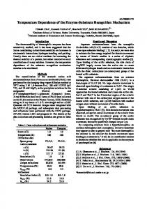
The distribution of particle sizes causes a temperature dependence of the coexistence of both (1) blocked and (2) superparamagnetic particles. The influence of superparamagnetic particles on the coercive field was explicitly taken into account by Kneller and Luborsky.7 They considered that the magnetization curves of components (1) and (2) are linear for H < HCB (see Fig. 1). Hence M1 = M r + (M r/HCB )H for component (1) and M2 = χS H for component (2), where M r is the remanence, H the applied magnetic field and χS the superparamagnetic susceptibility. These two components may be linearly superposed and the average coercive field becomes
hHC iT =
C.
Mr (T ) χS (T ) +
Mr (T ) HCB (T )
.
(7)
Determination of hHC iT
In order to obtain hHC iT by Eq. (7), three terms must be evaluated: Mr (T ), χS (T ), and HCB (T ) all determined from experiments. For the last two terms, a good determination of f (TB ) is needed. The isothermal remanent magnetization is related to f (TB ) according to:13 Z ∞ Ir (T ) = αMS f (TB )dTB (8) T
3
Magnetization M
Mr
C
H
blocked particles CB
superparamagnetic particles total magnetization
Magnetic Field H
FIG. 1: Contribution of the superparamagnetic particles to the coercive field.
Clearly the derivative of Eq. (8) is a direct measure of the blocking temperature distribution f (TB ) i.e., dIr /dT ∝ f (TB ). The superparamagnetic susceptibility has two contributions: isolated and groups of a few Co atoms, χSA (T ), and particles, χSP (T ). The later is the initial susceptibility in the low field limit given by MS2 V /3kB T . For a system with nonuniform particle sizes, it can be calculated as: Z V c(T ) MS2 χSP (T ) = V f (V )dV 3kB T 0 Z 25MS2 T TB f (TB )dTB , (9) = 3KT 0 where the linear relation between TB and V (Eq. (2)) was used to express χSP (T ) in terms of TB , and the critical volume Vc above which the particle is blocked. Thus, the superparamagnetic susceptibility can be written as Z 25MS2 T C χS (T ) = (10) TB f (TB )dTB + , 3KT 0 T where the second term is the contribution of groups of a few Co atoms defined in terms of the Curie constant C. Finally HCB (T ) is determined from the Eqs. (5) and (6). Alternatively, f (TB ) can also be determined from zero field cooled (ZFC) and field cooled (FC) magnetization experiments12 when one is sure that there are no blocked particles at the highest measuring temperature, which is not always the case. III.
EXPERIMENTAL
We have studied two Cu-Co ribbons of nominal composition Cu97 Co3 and Cu90 Co10 in the as cast form. These samples were prepared by melt spinning as described in reference 16. The hysteresis loops M (H) of these samples were measured in the temperature range from 2 to 300 K and maximum field of 90 kOe.
The temperature dependence of the coercive field, and remanent magnetization were determined from the hysteresis loops. The saturation magnetization was determined by extrapolation of M (1/H) for 1/H = 0, at 2 K. ZFC curves were measured cooling the system in zero magnetic field and measuring during warming with an external field applied. The FC curves were measured during the cooling procedure with field. The Ir (T ) curve was measured cooling the systems in zero magnetic field from room temperature. At each temperature the samples were submitted to a field of 7 kOe which gives a negligible remanent field in the superconducting magnet and is well above the field where the hysteresis loop closes. Following the same procedure used by Chantrell et al.13 , Ir (T ) was determined by waiting 100 s after the field is set to zero. All measurements were performed using a Quantum Design Physical Property Measurement System (PPMS) model 6000.
IV. A.
RESULTS AND DISCUSSION
Distribution of energy barriers and system nanostructure
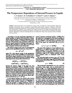
The morphology of a granular system consisting of magnetic precipitates plays an important role on the macroscopic behavior. Many efforts were made to investigate the morphology of granules in Cu-Co alloys. It is very difficult to use electron microscopy to identify Co granules in a Cu matrix due to the almost identical atomic scattering factor of Cu and Co atoms and very similar lattice parameter between the Cu matrix and Co granules31. Other experimental techniques could only be used to estimate the average size distribution25,26,32 . In many nanoparticle systems the experimental magnetization curves are remarkably well fitted using a superposition of properly weighted Langevin curves, usually considering a log-normal distribution.22 Making the assumptions that the magnetization of each spherical particle is independent of its volume, the particle size distribution may be obtained. In fact, the M (H) curves for the sample Cu90 Co10 shown in Fig. 2(a) exhibits a superparamagnetic shape, the same occurring also for Cu97 Co3 . However, M (H) is more sensitive to the average magnetic moment (or average particle size) than the width or distribution shape.23 For this reason the use M (H) to determine f (TB ) is not a good choice. In addition, a closer look to the small hysteresis shows that while the remanence decays with temperature, the coercive field at 20 K is smaller than at 4 and 300 K (see Fig. 2(b)). This issue will be discussed in next section. We first used ZFC/FC curves (shown in Fig. 3) as usually done to determine the distribution f (TB ). Is is clear that the warming and cooling curves do not close as to the highest measured temperature. The histeresis in the M (H) curve (see fig. 2 b) at 300 K show the presence of
4 blocked particles. The determination of the distribution f (TB ) using this ZFC/FC curves would clearly lead to an inaccurate result because it would neglect the remaining blocked particles above T = 330 K. We found thus better to determine the distribution by the use of eq. 8 and teh experimental remanence. 10 T = 300 K
+
�� � � 1−A 1 TB √ (11) exp − 2 ln2 2σ2 hTB2 i TB 2πσ2
The lines in Fig. 4 were obtained fitting the experimental data to the integrated Eq. (8) using the above f (TB ) distribution. The free parameters used in the fit were σ1 , hTB1 i, σ2 , hTB2 i and the weighting factor A, all shown in Table I. Since KV ∝ TB , f (TB ) represents the distribution of energy barriers.
M (emu/g)
5 1
I (T) / I (2K)
0
-5
r
a)
-80
-40
0
40
0.1 Cu
80
H (Oe)
Cu
Co
90
3
10
Calculated
0.01
a)
T = 4 K
2
Co
97
r
-10
T = 20 K
0.1
T = 300 K
0.01
0
B
f (T )
M (emu/g)
1
-1
1E-3
b) 1E-4
-2 -0.2
0.0
1E-5
0.2
b)
H (Oe)
1E-6 1
FIG. 2: (a) Hysteresis loop for the Cu90 Co10 as cast sample at room temperature. (b) A detail of the narrow hysteresis at different temperatures.
10
100
T (K)
FIG. 4: (a) Remanent magnetization for Cu97 Co3 (square symbols) and Cu90 Co10 (circles). (b) Distribution calculated using Eqs. (8) and (11).
0.35
Cu 0.30
Magnetization [emu]
H
Co
90
DC
10
We can see in Fig. 4(a) that the agreement between the theoretical and experimental curves is good for both samples. Figure 4(b) shows the distribution of energy barriers obtained from the derivative of the isothermal remanence decay (Eq. (8)). The obtained f (TB ) confirm the inhomogeneous magnetic nanostructure observed by other authors.24,25,26,27
as cast
= 100 Oe
0.25
0.20
0.15
0.10
0.05
0.00 0
50
100
150
200
250
300
Temperature [K]
FIG. 3: Zero field cooled and field cooled curves for the Cu90 Co10 as cast measured at HDC =100 Oe up to T = 330 K.
Figure 4(a) shows the temperature dependence of the isothermal remanence of Cu97 Co3 and Cu90 Co10 samples. Cu90 Co10 presents two inflexion points suggesting two mean blocking temperatures (hTB1 i and hTB2 i). This leads us to assume f (TB ) as being the sum of two lognormal distributions: �� � � A TB 1 2 √ f (TB ) = exp − 2 ln 2σ1 hTB1 i TB 2πσ1
TABLE I: Blocking temperature distribution parameters Sample σ1 < TB1 > (K) σ2 < TB2 > (K) A(%) Co3 Cu97 1.2 8.4 0.6 53 61 Co10 Cu90 0.7 2.7 1.4 128 78
Some characteristics of the nanostructure can be inferred from above results. For Cu90 Co10 there is a large number of small particles (small energy barriers) responsible for the low temperature maximum, and a few large particles responsible for second peak in the energy barrier (see Fig. 4(b)). For the less concentrated sample (Cu97 Co3 ), the energy barrier of the two groups of particles (small and large) is expected to be smaller than the observed in more concentrated sample, owing to the corresponding reduction in the particle sizes. However,
5 we observe that hTB1 i is bigger than for the more concentrated sample (see Table I). Such behavior can be related to the higher surface anisotropy as the particle size decreases.23
,
800
H
C
H
C
experimental
calculated ( ) C
T
400
The temperature dependence of the coercive field HC (T ) is shown in Fig. 5. While the more diluted sample presents the usual decrease with T , the Cu90 Co10 sample exhibits an unusual HC (T ) with a sharp decrease up to 20 K, followed by an increase and a maximum around 180 K. The solid lines were calculated by use of Eq. (7) with f (TB ) obtained previously and adjusting the anisotropy constant K in Eqs. (5) and (10). Some additional considerations has to be made to obtain a good agreement with the data. The straight calculation of HC (T ) gives the dashed line shown in Fig. 6. It is clear that a better agreement could be obtained by a horizontal shift in this plot. It is well known that barrier distributions f (TB ) are field dependent.12,28 The distribution of energy barriers obtained from magnetization measurements shows a temperature shift, which is a function of either the applied field or the magnetization state of the sample.12,29 Allia et al.18 have proposed that the effect of interparticle interactions can be pictured by the use of an additional temperature term in the Langevin function. In our case the results suggest to use f (γTB ) instead of f (TB ), were γ is an empirical parameter that takes into account the effect of random interactions. This leads to a better agreement, as shown by the dotted line curve. So far we did not take into account the Curie term in Eq. (10). By doing so, the agreement with experimental data becomes excellent as shown by the solid lines in Figs. 5 and 6 (for both samples). The best obtained parameters are shown in Table II. TABLE II: Best adjusted parameters
a) Cu
Co
b) Cu
Co
(Oe)
97
C
Coercive field
0
200
100 90
0
0
100
10
200
300
T (K)
FIG. 5: Coercive field HC vs. temperature for the two samples investigated: experimental (symbols) and calculated with the generalized model (line).
The interesting behavior of HC (T ) of the Cu90 Co10 sample can be understood in terms of χS (T ). Initially HC (T ) decreases with temperature due to the unblocking of the small particles (see Fig. 7). Then, thermal fluctuations leads to a decrease of χS and a consequent increase of HC with T until the large particles start to unblock and HC (T ) decreases again. In the other sample, unblocking occurs more smoothly in whole temperature range, due to the relative proximity of the hTB1 i and hTB2 i, and HC (T ) present the expected decrease with T (see Fig. 5(a)). The above description is particulary adequate for systems that present considerable interactions and deviations of HC (T ) around near hTB i. This was more evident in the Cu90 Co10 sample due to its unusual behavior. In this respect we present a comparison of different possible
Sample K (erg/cm3 ) C (emu*K/Oe*cm3 ) γ Co3 Cu97 as cast 5.0 ∗ 106 2.3 1.4 Co10 Cu90 as cast 3.2 ∗ 106 1.4 2.4
500 H
400
C
experimetal = 1 and
= 2.4 and
=
S
S
SP
= =
Sp
+
Sa
Sp
200
H
C
(Oe)
S
= 2.4 and
300
We can see in the Table II that K is smaller for the more concentred sample, which is consistent with the relative reduction of the surface anisotropy contribution with the size of the nanoparticles.23,30 Note that the Co3 Cu97 sample presents a higher concentration of isolated groups of a few Co atoms and smaller interaction parameter γ. The expected stronger interaction (and γ) in the Co10 Cu90 sample may also imply in a reduction of K, as suggested by the random anisotropy model.10 The application of this model to a system with a negligible interaction provides a good description of Hc(T) with a gamma temperature shift in the distribution equal to 1 (γ = 1).
3
H
B.
100
1
10
100 T (K)
FIG. 6: HC calculations and experimental data for Cu90 Co10 . The full line is the hHC iT obtained considering interaction and groups of a few Co atoms.
6 600 500
experimental
calculated
C
C
400
T
T
(T) S
1
200
S
H
C
(Oe)
3
(emu/Oe*cm )
300
100
0.1 1
10
100
T (K)
FIG. 7: Calculated χS (dotted line), hHC iT (solid line), and experimental data (open symbols) vs. temperature of the Cu90 Co10 sample.
(Oe) C
CB
B
using B
T
using
using
C
300
H
CB
C
T
T
B
200
B
T
1000
100
0
0
100
200
300
CONCLUSION
2000
using
(Oe)
H
V.
experimental
CB
C
H
H
H
400
and (4), that works for well isolated and narrow distributions of sizes.3 The dashed line is determined by considering the temperature dependent average blocking temperature (Eqs. (3) and (6)) and shows clearly the need to include the superparamagnetic correction. By considering further this correction with Eq. (4) and (7) the dashed-dotted line is obtained with an excellent agreement at low temperatures, where most of the particles are still blocked. When we take into account Eqs. (6) and (7), i.e., considering the temperature dependence of the average blocking temperature we obtain finally the solid line describing well the results in the whole temperature range.
0 400
T (K)
FIG. 8: Coercive field vs. temperature of the Cu90 Co10 sample: experimental (open squares), calculated hHC iT (solid and dotted-dashed lines), and HCB (dashed and dotted lines). For detail, see text.
We present a generalized model for the description of the thermal dependence of HC of granular magnetic systems. With this model we describe successfully the temperature dependence of the coercive field of Co-Cu samples. The contribution of superparamagnetic particles and the use of a temperature dependent average blocking temperature was shown to be important to describe the coercive field in a wide temperature range. The interactions among the particles were considered through an empirical multiplying factor γ as well as an effective size distribution. we believe that with this procedure most of the fine magnetic particle systems may be well described.
Acknowledgments
scenarios to explain the experimental data (see Fig. 8). Without taking into account the contribution (i) of superparamagnetic susceptibility of unblocked particles we obtain the curves indicated by the dotted and dashed lines. The dotted is the standard and widely used Eqs. (3)
1 2
3
4
5
6
7
8 9
L. N´eel, Ann. Geophysique 5, 99 (1949). J. L. Dormann, D. Fiorani and E. Tronc, Adv. Chem. Phys. 98, 283 (1997). C. Bean and J. D. Livingston, J. Appl. Phys. 30, 120S (1959). F. C. Fonseca, G. F. Goya, R. F. Jardim, R. Muccillo, N. L. V. Carreno, E. Longo and E. R. Leite, Phys. Rev. B 66,104406 (2002). X. Batlle, M. Garcia del Muro, J.Tejada, H. Pfeiffer, P. Gornert and E. Sinn, J. Appl. Phys. 74, 3333 (1993). D. Kechrakos and K. N. Trohidou, Phys. Rev. B 58, 12169 (1998). E. F. Kneller and F. E. Luborsky, J. Appl. Phys. 34, 656 (1963). H. Pfeiffer, Phys. Stat. Sol. (a) 118, 295 (1990). P. Vavassori, E. Angeli, D. Bisero, F. Spizzo, and F. Ronconi, Appl. Phys. Lett. 79, 2225 (2001).
This work was supported by Instituto de Nanociˆencias - Institutos do Milˆenio - CNPq, FUJB, CAPES and FAPERJ. The authors thank the project PRONEX/FINEP and Dr. R. S. de Biasi for helpful discussions.
10
11
12
13
14
15
16
17
18
W. C. Nunes, M. A. Novak, M. Knobel e and A. Hernando, J. Magn. Magn. Mater. 226-230, 1856 (2001). E. F. Ferrari, W. C. Nunes, and M. A. Novak, J. Appl. Phys. 86, 3010 (1999). N. Peleg, S. Shtrikman, G. Gorodetsky, and I. Felner, J. Magn. Magn. Mater. 191, 349 (1999). R. W. Chantrell, M. El-Hilo, And K. O’Grady, IEEE Trans. Magn. 27, 3570 (1991). W. S. D. Folly and R. S. de Biasi, Braz. J. Phys. 31 (3), 398 (2001). Janis Kliava, and Ren´e Berger, J. Magn. Magn. Mater. 205, 328 (1999). P. Allia, M. Knobel, P. Tiberto and F. Vinai, Phys. Rev. B. 52, 15398 (1995). J. Wecker, R. von Helmolt, L. Schultz, and K. Samwer, Appl. Phys. Lett. 62, 1985 (1993). P. Allia, M. Coisson, P. Tiberto, F. Vinai, M. Knobel, M.
7
19
20
21
22
23
24
25
A. Novak, and W. C. Nunes, Phys. Rev. B 64, 144420 (2001). E. C. Stoner and E. P. Wohlfarth, Philos. Trans. R. Soc. London A240, 599 (1948). M. El-Hilo, K. O’Grady and R. W. Chantrell, J. Magn. Magn. Mat., 114, 295 (1992) M. Blanco-Mantecn and K. O’Grady J. Magn. Magn. Mat., 203, 50 (1999) E. F. Ferrari, F. C. S. da Silva, and M. Knobel, Phys. Rev. B. 56, 6086 (1997). F. Luis, J. M. Torres, L. M. Garcia, J. Bartolome, J. Stankiewicz, F. Petroff, F. Fettar, J. L. Maurice, and A. Vaures, Phys. Rev. B 65, 94409 (2002). P. Panissod, M. Malinowska, E. Jedryka, M. Wojcik, S. Nadolski, M. Knobel, and J. E. Schmidt, Phys. Rev. B 63, 014408 (2000). A. Garc´ia Prieto, M. L. Fdez-Gubieda, C. Meneghini, A. Garc´ia-Arribas, and S. Mobilio, Phys. Rev. B 67, 224415 (2003).
26
27
28
29
30
31
32
A. L´ opez, F. J. Lzaro, R. von Helmolt, J. L. GarcaPalacios, J. Wecker, and H. Cerva, J. Magn. Magn. Mater. 187, 221 (1998). W. Wang, F. Zhu, W. Lai, J. Wang, G. Yang, J. Zhu, and Z. Zhang, J. Appl. Phys. 32, 1990 (1999). J. C. Denardin, A. L. Brandl, M. Knobel, P. Panissod, A. B. Pakhomov, H. Liu and X. X. Zhang, Phys. Rev. B 65, 064422(2002). M. Garcia del Muro, X. Batlle and A. Labarta, J. Magn. Magn. Mater. 221, 26 (2000). M. Respaud, J. M. Broto, H. Rakoto, A. R. Fert, L. Thomas, B. Barbara, M. Verelst, E. Snoeck, P. Lecante, A. Mosset, J. Osuna, T. O. Ely, C. Amiens and B. Chaudret, Phys. Rev. B 57, 2925 (1998). A. H¨ utten and G. Thomas, Ultramicroscopy 52, 581 (1993). R. H. Yu et al., J. Appl. Phys. 79(4), 1979 (1996).