PHYSICAL REVIEW E 82, 031111 共2010兲
Temperature for a dynamic spin ensemble Pui-Wai Ma,1,2 S. L. Dudarev,2 A. A. Semenov,1,* and C. H. Woo1,†
1
2
Department of Electronic and Information Engineering, The Hong Kong Polytechnic University, Hong Kong SAR, China EURATOM/CCFE Fusion Association, United Kingdom Atomic Energy Authority, Abingdon, Oxfordshire OX14 3DB, United Kingdom 共Received 30 March 2010; revised manuscript received 3 August 2010; published 7 September 2010兲 In molecular dynamics simulations, temperature is evaluated, via the equipartition principle, by computing the mean kinetic energy of atoms. There is no similar recipe yet for evaluating temperature of a dynamic system of interacting spins. By solving semiclassical Langevin spin-dynamics equations, and applying the fluctuation-dissipation theorem, we derive an equation for the temperature of a spin ensemble, expressed in terms of dynamic spin variables. The fact that definitions for the kinetic and spin temperatures are fully consistent is illustrated using large-scale spin dynamics and spin-lattice dynamics simulations. DOI: 10.1103/PhysRevE.82.031111
PACS number共s兲: 05.70.⫺a, 75.10.⫺b, 05.20.⫺y, 75.40.Gb
I. INTRODUCTION
Temperature is the most fundamental quantity in statistical mechanics. In macroscopic equilibrium thermodynamics it is evaluated by differentiating entropy with respect to the energy of the system 关1兴. In experiment and microscopic molecular dynamics simulations it is probed by monitoring the mean kinetic energy of atoms 关2–5兴 via T=
具p2i 共t兲典t 2 兺 2m . 3kBN i
共1兲
Equation 共1兲 refers to temperature associated with the excitation of translational degrees of freedom of particles described by an arbitrary Hamiltonian, where the kinetic energy EK is a quadratic function of the generalized momenta pi共t兲 关6兴. For a classical Hamiltonian ensemble of interacting particles, temperature can also be evaluated by computing the configuration averages of forces acting between the particles 关7–9兴. The fact that Eq. 共1兲 does not require differentiating the Hamiltonian makes it the most convenient and most often used recipe for monitoring temperature, through which the notion of temperature can be generalized even to nonequilibrium configurations, like the turbulent flow of liquids 关10兴 or high-energy collision cascades 关11兴. Generalizing Eq. 共1兲 to the case of a dynamic spin system is complicated by the fact that a generic spin Hamiltonian, such as the Heisenberg Hamiltonian H = − 21 兺i,jJijSi · S j, does not have the form to which the existing methods 关6–9兴 can be readily applied. Having a recipe for monitoring the spin temperature is necessary for analyzing a large variety of dynamic relaxation modes involving interactions between the spin, charge, and lattice degrees of freedom observed in experiments 关12–17兴 and simulations 关18–22兴. To understand these interactions, and to study the corresponding relaxation modes, it would be useful to have a method, conceptually similar to Eq. 共1兲, for evaluating the thermodynamic param-
*Permanent address: Institute for Nuclear Research, Russian Academy of Sciences, 60-th October Anniversary Prospect 7a, 117312 Moscow, Russian Federation. † Corresponding author:
[email protected] 1539-3755/2010/82共3兲/031111共6兲
eters of a spin ensemble, such as its temperature, directly from the variables characterizing its dynamic state. No such method presently exists. A canonical spin system can be brought into equilibrium with a thermostat using the Langevin stochastic exchange field algorithm 关23兴, subject to conditions imposed by the fluctuation-dissipation theorem 共FDT兲 关24–27兴. For example, in a spin-lattice dynamics simulation 关21兴, interaction with a thermostat, described by some suitably chosen Langevin stochastic forces, drives spin orientations asymptotically to the equilibrium Gibbs distribution. The inverse problem, namely, of how to evaluate the spin temperature from the known orientations of all spins, is still awaiting solution. In this paper, we derive an equation for the temperature of a spin ensemble expressed in terms of its dynamic state variables. The derivation involves investigating equilibrium solutions of semiclassical Langevin dynamic equations, and applying the FDT. The internal consistency between the formulas for spin temperature derived in this study, and for the kinetic temperature 关Eq. 共1兲兴 referring to the excitation of translational degrees of freedom, is illustrated using largescale spin and spin-lattice dynamics simulations.
II. LANGEVIN EQUATIONS AND THE SPIN TEMPERATURE A. Particle case
Before addressing the spin case, we first investigate the well-known limit where particles, not interacting between themselves, move under the action of random dissipative forces. The Langevin equations for freely moving atoms are 关24–27兴, dpi ␥l = − pi + fi共t兲, dt m
共2兲
where ␥l is the coefficient of dissipative drag for the translational, or lattice, degrees of freedom, and fi共t兲 are the deltacorrelated random forces satisfying conditions 具fi共t兲典 = 0 and 具f i␣共t兲f j共t⬘兲典 = l␦共t − t⬘兲␦ij␦␣, where Greek symbols ␣ and  denote the Cartesian components of a vector.
031111-1
©2010 The American Physical Society
PHYSICAL REVIEW E 82, 031111 共2010兲
MA et al.
冉
From the Langevin Eqs. 共2兲 it follows that
dE pi dpi U dRi + =兺 dt m dt Ri dt i
具p2i 典 ␥l具p2i 典 1 d具EK典 d =−兺 具pi共t兲 · fi共t兲典. = 兺 2 +兺 m dt dt i 2m i i m
=兺
共3兲 Here EK is the total kinetic energy of the system. The ensemble average is taken over all possible realizations of the stochastic forces. Substituting the formal solution of Eq. 共2兲 into 具pi共t兲 · fi共t兲典, we find 具pi共t兲 · fi共t兲典 = =
␥l m
冕
t
具pi共t⬘兲 · fi共t兲典dt⬘ +
0
冕
t
具fi共t⬘兲 · fi共t兲典dt⬘
0
3l , 2
i
冋冉 冉
冉
冊
具p2i 典 3l 2␥l d具EK典 =− − . 兺 dt m i 2m 4␥l
共5兲
At equilibrium, the system is stationary and the time derivative of the mean kinetic energy in the left-hand side of the equation must vanish. In this limit, the right-hand side of Eq. 共5兲 gives 具p2i 典 3l 3 1 = = kBT, 兺 N i 2m 4␥l 2
H=兺 i
dRi pi = . dt m The change of the total energy with respect to time is
共9兲
Adopting an approach similar to that outlined above, we consider a generic Heisenberg Hamiltonian describing a broad class of spin systems 关28兴, H=−
1 兺 JijSi · S j − Hext · 兺i Si , 2 i,j
共10兲
˜ is the effective external field, H ˜ is where Hext = −gBH ext ext the external magnetic field, g is the electronic g factor, B is Bohr magneton, Si is a spin vector, and Jij is the exchange interaction parameter involving spins i and j. Jij is a function of the geometry of the lattice and the electronic structure of the material 关28兴. The Hamiltonian equations of motion for dynamic variables Si can be derived using the Poisson brackets method 关29兴, namely, 1 dSi i = 关H,Si兴 = Si ⫻ dt ប ប
冉兺 k
冊
1 JikSk + Hext ⬅ Si ⫻ Hi . ប 共11兲
共7兲
where U共R兲 is the potential energy of interaction between the atoms, and R = 兵Ri其 are the coordinates of atoms. The corresponding Langevin equations of motion are
U ␥l dpi =− − pi + fi dt Ri m
␥lp2i pi · fi + . m2 m
B. Spin case
共6兲
where we equated the ensemble and the time average values, and evaluated the mean kinetic energy using the Gibbs distribution. The fact that l and ␥l are related via l = 2␥lkBT constitutes the FDT for the Langevin particles 关24–27兴. We note that Eq. 共6兲 has the same form as Eq. 共1兲, in agreement with the equipartition principle. Equation 共1兲 remains valid for the case of interacting particles. A Hamiltonian for interacting particles is p2i + U共R兲, 2m
冊
册
Comparing Eqs. 共9兲 and 共3兲, we see that the right-hand sides of both equations are identical. Using the same argument as for the case of non-interacting particles, we arrive at the relation between the momenta and kinetic temperature given by Eq. 共1兲.
共4兲
The first integral in the middle of Eq. 共4兲 vanishes because the argument of the integral 具pi共t⬘兲 · fi共t兲典 is equal to zero everywhere in the interval t⬘ 苸 关0 , t兲, except for the point t⬘ = t where it has a finite magnitude, unlike the second term, which integrates to give 3l / 2. Substituting Eq. 共4兲 into the last term of Eq. 共3兲 gives
冊
U ␥l U pi pi − − pi + fi + m Ri m Ri m
=兺 − i
冊
共8兲
Here the effective exchange field acting on spin i is Hi ⬅ 兺kJikSk + Hext. This effective field includes both the internal and external fields. We note that Eq. 共11兲 retains the same form for both the interacting, or non-interacting, spin system. In the presence of a random exchange field hi共t兲 the spin system becomes nonconservative. The Langevin equations of motion for spins take the form 关21兴 dSi 1 = 关Si ⫻ 共Hi + hi共t兲兲 − ␥sSi ⫻ 共Si ⫻ Hi兲兴, dt ប
共12兲
where ␥s is a dimensionless damping constant, which is introduced to compensate the effect of random noise hi共t兲 关21兴. The noise term hi共t兲 in Eq. 共12兲 is assumed to be delta correlated, satisfying the conditions 具hi共t兲典 = 0 and 具hi␣共t兲h j共t兲典 = s␦ij␦␣␦共t − t⬘兲. Here s is a parameter characterizing the amplitude of the random noise, and the Greek symbols ␣ and  again denote the Cartesian components of a vector. Equation 共12兲 is similar to that proposed by Brown 关23兴, who used a slightly different dissipation term −␥sបSi ⫻ dSi / dt. The fact that to a first approximation dSi / dt equals 共Si ⫻ Hi兲 / ប and that in Eq. 共12兲 the right-hand side does not contain the time derivative of dynamic spin variables, makes
031111-2
PHYSICAL REVIEW E 82, 031111 共2010兲
TEMPERATURE FOR A DYNAMIC SPIN ENSEMBLE
it consistent with the Langevin treatment of motion of particles described by Eq. 共8兲. The rate of variation of the ensemble-averaged total energy of the spin system, according to Eq. 共10兲 and 共12兲, is
冓
−
d共Si · S j兲 1 Jij 兺 2 i,j dt
冔 兺冓 冔 =−
Hi ·
i
=−
dSi dt
1 兺 关具Hi · 共Si ⫻ hi共t兲兲典 ប i
+ ␥s具兩Si ⫻ Hi兩2典兴.
共13兲
Here the ensemble average is taken over all possible realizations of the stochastic fields hi共t兲. Evaluating the averages according to 关30,31兴, we find 具Hi · 共Si ⫻ hi共t兲兲典 = −
s 具Si · Hi典, ប
Substituting this into Eq. 共13兲, we arrive at
冋
共14兲
册
s d具E典 1 = 兺 具Si · Hi典 − ␥s具兩Si ⫻ Hi兩2典 . dt ប i ប
共15兲
At thermal equilibrium, the system is stationary and the lefthand side of Eq. 共15兲 must vanish. Since s and ␥s are related by the FDT condition s = 2␥sបkBT 共see Ref. 关23兴 and Appendix兲, Eq. 共15兲 leads to the following equation for the spin temperature, expressed in terms of dynamic spin variables Si共t兲:
T=
s 2␥sបkB
冓兺 冔 冓兺 冓兺 冔 冓兺 兩Si ⫻ Hi兩2
兩Si共t兲 ⫻ Hi共t兲兩2
i
=
i
=
2kB
Si · Hi
i
2kB
i
Si共t兲 · Hi共t兲
冔 冔
t
.
t
共16兲 Equation 共16兲 is the central result of this paper. In deriving this equation we used the fact that averaging over all the possible realizations of the stochastic field hi共t兲 is equivalent to averaging over the statistical ensemble. Since Jij are parameters characterizing a given material, the temperature T of a spin system in Eq. 共16兲 is completely determined by the statistical distribution of the spins, in exactly the same way as the temperature of a system of moving particles is determined by its dynamics in Eq. 共1兲. A striking difference between Eq. 共16兲 and 共1兲, however, is that the spin temperature defined by Eq. 共16兲 can in principle be positive or negative, in agreement with Ref. 关32兴 共the latter case is realized, for example, if the orientations of spins Si are opposite to those of the effective fields Hi兲, whereas the kinetic temperature Eq. 共1兲 for an atomic ensemble is positive definite. Of course, in equilibrium the temperature of a spin system is equal to that of the lattice, and has to be positive. We also note that since the concept of temperature is thermodynamic, one needs to exercise caution when applying it to a non-equilibrium configuration. The issue of how to define temperature for a nonequilibrium situation is controversial 关9兴 and is beyond the scope of the present paper. Nevertheless, under conditions that make local equilibrium a valid
FIG. 1. 共Color online兲 Evolution of temperature for a dynamic spin system interacting with a Langevin thermostat. Asymptotically, the spin temperature given by Eq. 共16兲 approaches the temperature of the thermostat.
assumption, such as in the case where the global rate of energy change is much slower than that of the local equilibration processes, one may still assign the notion of temperature to a local dynamic set of variables according to Eq. 共16兲. In such cases Eq. 共15兲 shows that the empirical temperature assigned in this way still satisfies the fluctuation-dissipation condition, as required for a system in thermal equilibrium in that instance. III. THREE CASE STUDIES
In what follows, we consider three examples where the spin temperature, evaluated using Eq. 共16兲, can be compared with what is expected in terms of evolution and relaxation of the system. In the first case study, spin-dynamics 共SD兲 simulations are performed for bcc iron, using the exchange coupling parameters Jij chosen for ferromagnetic BCC iron according to Ref. 关21兴. We consider a spin ensemble realized on a 20a ⫻ 20a ⫻ 20a 共a = 2.8665 Å兲 bcc lattice containing 16 000 atomic spins 关21,33兴, with periodic boundary conditions applied in the x, y, and z directions. The initially collinearly ordered spin system is heated up and maintained at various preset temperatures by a Langevin thermostat 关21兴. No external field is applied. The dynamic temperatures of the spin systems evaluated using Eq. 共16兲 are plotted as functions of time in Fig. 1. In each simulation, the spin temperature defined by Eq. 共16兲 can be seen to rise from 0 K to an asymptotic value equal to the temperature of the canonical spin system as preset by the thermostat. The temperature fluctuations seen in Fig. 1 are due to limitations associated with the finite simulation cell size. Interestingly, this example suggests that if the temperature transient is sufficiently slow, Eq. 共16兲 may also be used to monitor the thermal equilibration process of the spin system similarly to Eq. 共1兲, the use of which in molecular dynamics simulations for this purpose is well established. In the second case study, we perform spin-lattice dynamics 共SLD兲 simulations 关21,33兴 for a spin-lattice system with the rigid-lattice constraint removed. The temperature of the spin subsystem is controlled with a Langevin thermostat, but the temperature of the lattice is left unconstrained, with parameter ␥l set to zero. The lattice and spin subsystems are
031111-3
PHYSICAL REVIEW E 82, 031111 共2010兲
MA et al.
FIG. 2. 共Color online兲 Lattice temperature 关Eq. 共1兲兴 plotted against spin temperature 关Eq. 共16兲兴 at equilibrium for a series of spin-lattice dynamics simulations. The Langevin thermostat is applied only to the spin subsystem. No temperature control applied to the lattice subsystem. Inset: the corresponding spin-lattice relaxation dynamics.
dynamically coupled via the coordinate-dependent exchange coupling function Jij共R兲 in the Heisenberg Hamiltonian Eq. 共10兲. We anticipate that at equilibrium the spin temperature, evaluated using Eq. 共16兲, and the lattice temperature, evaluated using Eq. 共1兲, must be equal. Using the same 16 000 atoms simulation cell as before, and applying the stress-free boundary conditions, we equilibrate the spin-lattice system. The inset in Fig. 2 shows the results of “temperature measurements” involving Eq. 共1兲 and 共16兲 for the lattice and spin systems performed during the thermalization process. These “measured” temperatures can be seen to separately approach the temperature of the spin thermostat. At t = 1.5 ns, we switch off the spin thermostat, turning the spin-lattice system into a microcanonical, i.e., an NVE, ensemble. The temperatures measured by Eq. 共1兲 and 共16兲 can be seen to remain steady, fluctuating about their average values. We note that these fluctuations are not related to the coupling between the lattice and the spin subsystems, but are intrinsic due to the large multiplicity of states of the spin system which have the same total energy but different spin orientations. In this regard, basic thermodynamics dictates that the temperature is determined by the change in the number of such states, i.e., the entropy, as a function of the energy of the system. We note that this is true for the fluctuations of both the spin and the lattice system; no matter whether they are coupled or decoupled. Figure 2 shows the average temperatures and their standard deviations for the lattice and the spin subsystems according to Eq. 共1兲 and 共16兲. The 45° straight line on which the data points lie shows very well that these two temperatures are equal at equilibrium and that Eq. 共1兲 and 共16兲 are consistent with each other. Finally, we consider the microcanonical relaxation of an initially spatially and thermally heterogeneous spin system. The initial condition for the simulation illustrated in Fig. 3 is set by bringing into contact the two spin subsystems equilibrated at 300 and 800 K, respectively, occupying the left and right halves of the simulation cell, subject to periodic boundary conditions. Experimentally, a nonequilibrium spin configuration similar to that shown in Fig. 3 can be generated using a laser or a microwave pulse. The evolution of the spin system is followed using a microcanonical spin dynamics
FIG. 3. 共Color online兲 Relaxation dynamics for a spin system with an initial temperature gradient. Evolution of the system is followed using microcanonical spin dynamics simulations. The local spin temperature 关Eq. 共16兲兴 is plotted as a function of the distance to the interface between the two initially separate parts of the system. The profiles reach equilibrium on the time scale of ⬃10 ps.
simulation. Since the total energy is conserved, the equilibration of the spin system takes place through the energy and angular momentum exchange between the neighboring volumes. In the simulation, the local energy, temperature 关defined according to Eq. 共16兲兴, and magnetization are evaluated for each atomic layer parallel to the interface between the two subsystems. The profiles of the local temperatures are shown in Fig. 3. All the three quantities follow similar trends, approaching the equilibrium and becoming spatially homogeneous at the temperature of ⬃550 K on the time scale of approximately 10 ps. This simulation shows that the spin temperature, defined by Eq. 共16兲, provides a useful means for monitoring the relaxation processes in the spin subsystem, similar to the way in which the notion of the local lattice temperature Eq. 共1兲 is applied to understanding the microscopic dynamics of turbulence 关10兴 or high-energy collision cascades 关11兴. IV. SUMMARY AND CONCLUSIONS
So far, there has been no practical recipe available for relating the temperature and the dynamic state of an ensemble of interacting spins. This issue is becoming increasingly important, as large scale simulations of spin ensembles evolve into tools for predictive exploration of magnetic phenomena on the nanoscale. This paper offers a closed-form expression that can be used for evaluating the thermodynamic temperature for a system of interacting spins in terms of the ensemble means of combinations of spin vectors. This expression was derived by solving the semi-classical Langevin-type equations of motion at equilibrium for the spins, and by using the fluctuation-dissipation theorem. The internal consistency between our spin-temperature expression 关Eq. 共16兲兴 and the kinetic lattice temperature expression 关Eq. 共1兲兴 is proven for the three case studies involving spin and spin-lattice dynamics simulations. In the first case, spin dynamics simulations of thermalization processes show that the spin temperature calculated according to Eq. 共16兲 asymptotically approaches that of the thermostat, in agreement with expectations. In the second example, the spin and the lattice
031111-4
PHYSICAL REVIEW E 82, 031111 共2010兲
TEMPERATURE FOR A DYNAMIC SPIN ENSEMBLE
degrees of freedom are allowed to interact, and direct spinlattice dynamics simulations show that spin temperature, defined in terms of spin dynamic variables, is fully consistent with the lattice temperature defined in terms of kinematic momenta. In the third case study, we investigate the microcanonical relaxation of an initially spatially and thermally heterogeneous spin system. The equilibrium temperature profile, which can only be obtained via Eq. 共16兲 in this case, agrees with expectations. Through this analysis, we prove that the notion of dynamic spin temperature offers a useful insight into the microscopic dynamics of relaxation of an initially spatially heterogeneous nonequilibrium system.
and diffusion coefficients, respectively. The upper-case Greek indexes ⌰ and ⌽ refer to the Cartesian components of a vector or a tensor. According to Brown 关23兴, the drift and diffusion coefficients can be expressed in terms of W0 and G = as
G ␣⌽ 1 A␣ = F␣ + s 兺 G⌰⌽ 2 ⌰,⌽ S⌰
共A3兲
B␣ = s 兺 G␣⌰G⌰ . ⌰
After some algebra, we arrive at ACKNOWLEDGMENTS
This project was initiated and funded by Grants No. 532008 and No. 534409 from the Hong Kong Research Grant Commission. It is also partially funded by the United Kingdom Engineering and Physical Sciences Research Council under Grant No. EP/G003955, and by the European Communities under the contract of Association between EURATOM and CCFE. P.-W.M. gratefully acknowledges European Fusion Development Agreement 共EFDA兲 for support. APPENDIX
The fluctuation and dissipation forces drive the spin ensemble asymptotically to equilibrium by changing the spin orientations. In principle, one could derive the FDT condition for the Langevin equation of motion for spins 关Eq. 共12兲兴 following the procedure described by Brown 关23兴. Here, we provide a simple derivation that proves the fluctuationdissipation relation 共FDR兲. We investigate the case of a single spin interacting with stationary external field. The Langevin equation of motion for a single spin in an external field, which resembles Eq. 共12兲, has the form dS 1 = 兵S ⫻ 关Hext + h共t兲兴 − ␥sS ⫻ 共S ⫻ Hext兲其. dt ប
1 s A = 关S ⫻ Hext − ␥sS ⫻ 共S ⫻ Hext兲兴 − 2 S ប ប 2 2 B␣ = s共␦␣兩S兩 − S␣兲/ប .
It should be noted that not only ␥s, but also s enter in the drift coefficient A␣. In the lattice case, only ␥l enters the expression for A␣ and only l enters B␣. Since random noise is delta correlated, and all the components of the linear momenta are independent, noise can in no way interact with other components of the momenta, and it does not enter the drift term. In the spin case, the effect of random noise goes into the drift term due to the presence of the cross product in the equations of motion, or equivalently the rotation nature of the spin motion. This allows the interaction of the noise at the current instant with the previous instant through other components of the spin vector. In thermal equilibrium 共i.e., W / t = 0兲, we identify the energy distribution for the spin system with the Gibbs distribution W = W0 exp共−H / kBT兲 where W0 is a normalization constant and H = −S · Hext. Substituting the Gibbs distribution into the Fokker-Planck equation, we find
冉
W 1 s = − 2␥s t ប បkBT
共A1兲
It can be rearranged into a sum of terms involving, or not = · h, where F involving, random noise, i.e., S˙ = F + G = is a tensor with com= 关S ⫻ Hext − ␥sS ⫻ 共S ⫻ Hext兲兴 / ប and G ponents G␣␣ = 0, G␣ = −S␥ / ប, and G␣␥ = S / ប. The lowercase Greek indices ␣, , and ␥ satisfy the cyclic permutation relations for x, y, and z. We map the equations of motion to the Fokker-Planck equation 关26,27兴,
2 1 W =−兺 共A⌰W兲 + 兺 共B⌰⌽W兲, 2 ⌰,⌽ S⌰ S⌽ t ⌰ S⌰ 共A2兲 where W is the energy distribution function, A␣ 1 1 = lim⌬t→0 ⌬t 具⌬S␣典 and B␣ = lim⌬t→0 ⌬t 具⌬S␣⌬S典 are the drift
共A4兲
冊冉
冊
1 兩S ⫻ Hext兩2 − S · Hext W. 2kBT 共A5兲
Since the second bracket in the right-hand side contains variable quantities, the condition of thermal equilibrium implies that the right-hand side of Eq. 共A5兲 vanishes if and only if
s = 2␥sបkBT.
共A6兲
This means that if s and ␥s are related by Eq. 共A6兲, the Gibbs distribution solves the Fokker-Planck equation. This proves the FDR. The derivation being presented here can be generalized to the case of many-body interacting spins. In fact, the FDR should not change for an interacting spin system, provided that the way how the fluctuation and dissipation force enters the equations of motion remains the same.
031111-5
PHYSICAL REVIEW E 82, 031111 共2010兲
MA et al. 关1兴 L. D. Landau and E. M. Lifshitz, Statistical Physics, Part 1, 3rd ed. 共Pergamon, New York, 1980兲. 关2兴 M. P. Allen and D. J. Tildesley, Computer Simulation of Liquids 共Oxford University Press, New York 1987兲. 关3兴 C. Monroe, W. Swann, H. Robinson, and C. Wieman, Phys. Rev. Lett. 65, 1571 共1990兲. 关4兴 A. P. Mosk, Phys. Rev. Lett. 95, 040403 共2005兲. 关5兴 H. Berro, N. Fillot, and P. Vergne, Tribol. Lett. 37, 1 共2010兲. 关6兴 H. H. Rugh, Phys. Rev. Lett. 78, 772 共1997兲. 关7兴 O. G. Jepps, G. Ayton, and D. J. Evans, Phys. Rev. E 62, 4757 共2000兲. 关8兴 C. Braga and K. P. Travis, J. Chem. Phys. 123, 134101 共2005兲. 关9兴 J. Casas-Vázquez and D. Jou, Phys. Rev. E 49, 1040 共1994兲; Rep. Prog. Phys. 66, 1937 共2003兲. 关10兴 D. J. Evans and G. P. Morriss, Phys. Rev. Lett. 56, 2172 共1986兲. 关11兴 A. Caro and M. Victoria, Phys. Rev. A 40, 2287 共1989兲; D. M. Duffy and A. M. Rutherford, J. Phys.: Condens. Matter 19, 016207 共2007兲; A. M. Rutherford and D. M. Duffy, ibid. 19, 496201 共2007兲. 关12兴 E. Beaurepaire, J.-C. Merle, A. Daunois, and J.-Y. Bigot, Phys. Rev. Lett. 76, 4250 共1996兲. 关13兴 A. Scholl, L. Baumgarten, R. Jacquemin, and W. Eberhardt, Phys. Rev. Lett. 79, 5146 共1997兲. 关14兴 G. P. Zhang, W. Hübner, G. Lefkidis, Y. Bai, and T. F. George, Nat. Phys. 5, 499 共2009兲. 关15兴 J.-Y. Bigot, M. Vomir, and E. Beaurepaire, Nat. Phys. 5, 515 共2009兲. 关16兴 C. Stamm, T. Kachel, N. Pontius, R. Mitzner, T. Quast, K. Holldack, S. Khan, C. Lupulescu, E. F. Aziz, M. Wietstruk, H.
A. Dürr, and W. Eberhardt, Nature Mater. 6, 740 共2007兲. 关17兴 E. Carpene, E. Mancini, C. Dallera, M. Brenna, E. Puppin, and S. De Silvestri, Phys. Rev. B 78, 174422 共2008兲. 关18兴 M. Fähnle, R. Singer, D. Steiauf, and V. P. Antropov, Phys. Rev. B 73, 172408 共2006兲. 关19兴 W. Hübner and G. P. Zhang, Phys. Rev. B 58, R5920 共1998兲. 关20兴 B. Koopmans, J. J. M. Ruigrok, F. Dalla Longa, and W. J. M. de Jonge, Phys. Rev. Lett. 95, 267207 共2005兲. 关21兴 P. W. Ma, C. H. Woo, and S. L. Dudarev, Phys. Rev. B 78, 024434 共2008兲; also in Electron Microscopy and Multiscale Modeling, edited by A. S. Avilov et al., AIP Conf. Proc. No. 999 共AIP, New York, 2008兲, p. 134. 关22兴 J. L. García-Palacios and F. J. Lázaro, Phys. Rev. B 58, 14937 共1998兲. 关23兴 W. Fuller Brown, Jr., Phys. Rev. 130, 1677 共1963兲. 关24兴 R. Kubo, Rep. Prog. Phys. 29, 255 共1966兲. 关25兴 S. Chandrasekhar, Rev. Mod. Phys. 15, 1 共1943兲. 关26兴 R. Zwanzig, Nonequilibrium Statistical Mechanics 共Oxford University Press, New York, 2001兲. 关27兴 N. G. Van Kampen, Stochastic Processes in Physics and Chemistry 共North-Holland, Amsterdam, 1981兲. 关28兴 I. Turek, J. Kudrnovsky, V. Drchal, and P. Bruno, Philos. Mag. 86, 1713 共2006兲. 关29兴 L. A. Turski, Phys. Rev. A 30, 2779 共1984兲. 关30兴 V. I. Klyatskin, Statistical Description of Dynamical Systems with Fluctuating Parameters 共Nauka Publishers, Moscow, 1975兲. 关31兴 M. Tokuyama, Physica A 102, 399 共1980兲; 109, 128 共1981兲. 关32兴 E. M. Purcell and R. V. Pound, Phys. Rev. 81, 279 共1951兲. 关33兴 P. W. Ma and C. H. Woo, Phys. Rev. E 79, 046703 共2009兲.
031111-6