1
Template Matching via l1 Minimization and Its Application to Hyperspectral Data Zhaohui Guo and Stanley Osher
Abstract—Detecting and identifying targets or objects that are present in hyperspectral ground images are of great interest. Applications include land and environmental monitoring, mining, military, civil search-and-rescue operations, and so on. We propose and analyze an extremely simple and efficient idea for template matching based on l1 minimization. The designed algorithm can be applied in hyperspectral classification and target detection. Synthetic image data and real hyperspectral image (HSI) data are used to assess the performance, with comparisons to other approaches, e.g. spectral angle mapper (SAM) and adaptive coherence estimator (ACE). We demonstrate that this algorithm achieves excellent results with both high speed and accuracy by using Bregman iteration. Index Terms—Hyperspectral, template matching, Bregman, l1 minimization.
I. I NTRODUCTION
I
N recent decades, hyperspectral remote sensing technology has become highly developed. Remote sensing can be used to collect the reflective spectrum of the objects in a scene at specific wavelengths simultaneously, resulting in hundreds of digital images. The data collected from a hyperspectral sensor contains not only the visible spectrum, but also ultraviolet and infrared ranges as well. It is common to list the hyperspectral data in a three-dimensional array or “cube”, with the first two dimensions corresponding to spatial dimensions and the third one corresponding to the spectrum. Since the distinct materials leave different spectral signals, each of which is known as the spectral signature, there has been an increasing demand in using spectral imagery to detect specific objects or targets of interest. Target detection is one of the most important hyperspectral image (HSI) applications based on materials’ spectral signatures, as is classification. In hyperspectral classification and especially target detection, the main task is to find the spatial pixels in threedimensional hyperspectral cube data for some given spectral signals of interest. However, this becomes difficult because of the uncertainty and variability of each material’s spectral signature. The difficulties include the noise from atmospheric conditions, sensor influence, location, illumination and so on, all of which depend on when and where the image was taken. Another disadvantage is that the same materials will not generate identical spectral curves for physical reasons, especially between the laboratory data and actual image data. Occasionally, two different materials might unexpectedly reflect Research supported by the Department of Defense. Z. Guo and S. Osher are with the Department of Mathematics, University of California, Los Angeles, CA 90095, USA (e-mail:
[email protected];
[email protected]).
similar spectral signals, like two different types of vegetation. Additionally, the low resolution of the hyperspectral image make it reasonable to accept the fact that a single pixel may be composed of several different materials. These are usually called mixed pixels. The spectral signal of this mixed pixel is totally different from the spectrum of the pure materials. All of these facts increase the difficulties in processing HSI data, making classification and target detection highly challenging problems. Previous work dealing with hyperspectral target detection includes both statistical and geometrical approaches. Statistical approaches are mostly based on the assumption that HSI data can be represented by a multivariate normal distribution. The statistical models employing two hypotheses H0 and H1 corresponding to given material absent and present are well known as the likelihood ratio (LR) test (optimum) and generalized-likelihood ratio test (GLRT) [1], [2] (adaptive) detectors. Some other related algorithms with details can be found in [3], [4], [5], [6], [7]. Also, adaptive coherence estimator (ACE) [8] as an extension of generalized-likelihood ratio test (GLRT), employs a covariance matrix to identify the background, and achieves better result. However, in these models, prior knowledge including background information has to be obtained from training data, like the covariance matrix of the background. Where to set the threshold towards a reasonable compromise between probability of detection and probability of false alarms is also a question. In practice, there still exist serious challenges. The spectral angle map (SAM) [9], and the adaptive subspace detector (ASD) [10], [11] are representative geometrical algorithms. In addition, similar methods based on hypotheses and GLRT include the matched subspace detector [12], and matched filter algorithms, which in turn include orthogonal subspace detector (OSD) [12], [13] and spectral matched filter (SMF) [14], [15]. Many classical hyperspectral classifiers have been used in remote sensing, including minimum distance to mean (MD), spectral angle mapper (SAM), maximum likelihood (ML), fisher linear likelihood and so on. In order to reduce the error, classification is usually performed in the Principal Component Analysis (PCA) and Generalized Eigenvalue (GEV) dimensionality reduced domains. Our method resembles SAM, but has an l1 sparsity term which seems to improve the performance. We will discuss this further. The paper is organized as follows. A brief introduction of Bregman methods for l1 minimization and the algorithm for template matching are presented in Section II. In Section III, we apply the proposed algorithm to a simulated data
2
set and the real HSI image data sets. Comparisons with classical algorithms, spectral angle map (SAM) and adaptive coherence estimator (ACE), are presented based on receiver operating characteristic (ROC) curves to show the obtained improvements. Finally, conclusions are given in Section IV. II. T EMPLATE M ATCHING A PPROACH AND A LGORITHMS In this section, we first briefly introduce the concept of Bregman iteration [16], and two different algorithms: linearized Bregman[17], [18], [19], [20] and split Bregman [21], [22], then present our algorithm for template matching. This is done to give simple and effective methods for potential users to do the l1 minimization. A. Bregman Iteration and Algorithms Bregman methods [23] applied to image processing [16] and compressive sensing (CS) [24], [19], [21], [20], [25] are an emerging field for solving sparse reconstruction and improving signal and image enhancement. Bregman iteration is based on the definition of Bregman distance. The Bregman distance for a convex function J(u) defined in Rn → R ∪ {+∞} is given as: DpJ (u, v) = J(u) − J(v)− < p, u − v >, where p ∈ ∂J is a subgradient of J at the point v, and < ·, · > is used as the inner product. In general Bregman distance shows the closeness between two points u and v, even though it doesn’t satisfy the symmetry and triangle inequality properties of usual distance. Consider a general constrained minimization problem: minu J(u) s.t. H(u) = 0, or H(u) < σ,
(1)
where H(u) is convex and differentiable energy function with zero as its minimum value. σ is the noise measure coming from the original problem. We transform it to an unconstrained minimization problem using: minu { µJ(u) + H(u) }. (2) µ > 0 works as penalty weight. Bregman iteration solves a related problem iteratively by replacing J(u) by DpJk (u, uk ): ½ k+1 u = argminu (µDpJk (u, uk ) + H(u)), (3) k+1 p = pk − ∂H(uk+1 ), where ∂H(uk+1 ) is a subgradient of H at uk+1 . The problems under consideration here use H(u) = 12 ||Au − f ||22 for some linear operator A and vector f . These can be easily solved by two related algorithms: linearized Bregman and split Bregman. Linearized Bregman [17], [18], [19], [20] was proposed to solve the basis pursuit problem minu |u|1 s.t. Au = f,
(4)
where A ∈ Rm×n , f ∈ Rn be given, and m < n. The related unconstrained minimization problem is 1 minu { µ|u|1 + ||Au − f ||22 }. 2
(5)
The algorithm can be written iteratively by introducing an auxiliary variable v k : ½ k+1 v = v k − AT (Auk − f ), (6) k+1 u = δ · shrink(v k+1 , µ), where u0 = v 0 = 0, δ > 0 works as define k+1 −µ : v 0 : shrink(v k+1 , µ) = k+1 v +µ : ½ k+1 v −µ + k+1 shrink (v , µ) = 0
the step size, and we v k+1 > µ −µ ≤ v k+1 ≤ µ , v k+1 < −µ (7) : v k+1 > µ , (8) : v k+1 ≤ µ
where the shrink + is designed for computing nonnegative solutions. The algorithm is solved iteratively and can be terminated when the noise level σ is reached. It is shown in practice to be a simple and fast algorithm when an appropriate positive value of δ is chosen. This method converges to a solution[17] of 1 u = argmin{ µ|u|1 + ||u||22 } s.t. Au = f. (9) 2δ If δµ is large enough, the solution is an exact solution of the basis pursuit problem, see [26]. Split Bregman was first introduced by Goldstein and Osher [21] for solving l1 , TV, and related regularized problems and applied to various imaging problems[22], [25], [27]. To solve our unconstrained sparse reconstruction problem, the iteration is generated by using an auxiliary variable d, and given by λ 1 (u, d) = argmin{ µ|d|1 + ||Au−f ||22 + ||d−u||22 }. (10) 2 2 µ, λ > 0 work as penalties balancing the energy functions. Optimization is performed in an alternating fashion: ½ k+1 u = argmin{ λ2 ||Au − f ||22 + 12 ||dk − u − bk ||22 }, k+1 d = argmin{ µ||d||1 + 21 ||d − uk+1 − bk+1 ||22 }. (11) In this fashion, we“split” the l1 and l2 components of the minimization function. bk comes from “adding back the error”. Thus we can perform this minimization scheme as follows: initially set u0 = b0 = d0 = 0; f 0 = f , then update the variables by inner and outer iterations. The inner iteration is given as k+1 = (λAT A + I)−1 (λAT f n − bk + dk ), v k+1 b = bk + v k+1 − dk , (12) k+1 d = shrink(v k+1 + bk+1 , µ), in which shrink is defined in (3) (or (4) for the nonnegative case). we know that ||v k − un+1 || converges monotonically as k increases to infinity, as does ||v k − dk ||. The outer iteration is given as f n+1 = f n + f − Aun+1 . In practice, we use a fixed number of inner iterations, usually 5-10 steps. It is proved in [25] that the iteration converges even with only one inner step. This is called Bregmanized operator splitting (BOS). λ is required to be smaller than ||AT1A||2 to ensure the convergence of iteration. To speed up the convergence, we choose λ larger, around ||A100 T A|| . µ is a parameter that balances the l1 and l2 2
3
components. It is determined by the actual data. This turns out to be a very efficient method for l1 minimization, and we will use it below. If A is fixed and saved as a prior knowledge, (λAT A+I)−1 in (12) could be precomputed, resulting in run-time savings. However, the size of square matrix (λAT A + I) is dependent on the number of columns of A. Note that if Au = f is underdetermined and the number of column is very large, it is impractical to compute the inverse. An alternative method could be used here. Instead of solving v k+1 = (λAT A + I)−1 (λAT f n − bk + dk ) in (12), we insert two new variables y and g, g = λAT f n − bk + dk , y = (λAAT + I)−1 Ag, k+1 v = g − λAT y,
(13)
(14)
Using (14), the computation of inverse matrix is only done for a much smaller size matrix of (λAAT + I). Equivalence between (13) and (14) can be proved easily through a few steps of simple linear transformation. B. Template Matching Approach The template matching approach basically employs the l1 sparsity idea arising in compressed sensing [24], [28]. Suppose the hyperspectral image is given as N by N pixels, each containing an M channel spectrum (a spectral band), as a three-dimensional cube. We aim to locate the pixels of interest in the image corresponding to a given spectral signal f , which is a specific object containing the same M channel spectrum. We arrange A as an M by N 2 matrix, with generally M < N 2 . The signals ai,1≤i≤N 2 is the column of the spectrum matrix A, and corresponds to each pixel in the hyperspectral image. f is a given material’s spectral signal. The aim is to 2 find the nonzero component ui in the solution u ∈ RN of the constrained minimization problem: minu |u|1 s.t. ||Au − f ||2 < σ and u ≥ 0.
(15)
The ui,1≤i≤N 2 corresponds to the same pixel as ai . By searching for the nonzero component ui , we can locate the pixels of interest. With the introduction of l1 minimization, the algorithm becomes much more robust. Furthermore, Au = f is an underdetermined linear system and has at least one solution. There are many methods proposed to do this numerical computation. In this paper, we apply split Bregman to the following unconstrained minimization problem. 1 (16) minu { µ|u|1 + ||Au − f ||22 } s.t. u ≥ 0. 2 To get a nonnegative solution, shrink + should be employed in the algorithm. In practice, the solution for hyperspectral data turns out to be nonnegative even without the nonnegative constraint employed here because of the nonnegativity of the data. Surprisingly this simple idea works well because the l1 norm term forces the energy to find a sparse solution u for µ large enough, which will enable the solution to pick up
the matching pixels compared with the desired spectral signal f , and ignore nonmatching pixels. In detection applications, it is highly possible that the matching pixels are sparsely distributed, or the number of matching pixels is limited, which makes the problem difficult and interesting. The sparseness of the matching pixels means the sparseness of u. We say that given a proper value of µ, the solution results in u with a limited number of positive components, which just correspond to the matching pixels in the image with a given spectral signal f. However, even in the nonsparse (numerous) case, this also works well. We can easily illustrate this by a simple clean case of classification. We randomly choose n pixels in the image and assign them to be the material of interest. We assume the spectrum of these pixels identically equal to f , or proportional to f , which means kf , 0 < k < 1 works as a simulated shadow effect. After solving the l1 minimization problem, we get a sparse solution u with each nonzero component ui corresponding to exact the same n pixel we chosen. The values of these ui are, close to n1 after normalization. Of course, it does make sense since the algorithm aims to find the proper solution u to make ||Au − f ||2 as small as possible, while ignoring the spectral signatures distinct from f . In the actual computation, the only significant parameter that should be considered is the quantity µ to control the sparsity of the solution, while λ could be chosen fixed. There exists a suitable range of µ for each set of HSI data. In detection applications, the number of matching pixels is much smaller than the total number of image pixels, µ could vary in a much large range. The result wouldn’t be affected so much. But in the classification case, sometimes the number of matching pixels is numerous, the result depends on µ largely. If µ is chosen to be too large, the algorithm will only identify a few correct matches. To deal with this problem, we can remove the detected matches and do the algorithm again on the remaining pixels using a new matrix with fewer columns. Simultaneously, if the background spectral signatures are quite distinct from f , we get no false alarms despite the change of µ. Otherwise, it will depend on µ. However, in practice the number of incorrect matches turns out to be much fewer than the number of correct matches, and the coefficients ui of most incorrect matches are much smaller than those of the correct matches, usually by 1 or 2 orders of magnitude. Thus we can set up a simple threshold to identify the correct result. In contrast to the other methods, the algorithm involves neither any requirement of background information nor the assumption of multivariate normal distribution of the background and designed material during the whole computation process. Only the spectrum of material of interest is needed in the algorithm. The method can deal with the case when the matches are sparse or numerous and when background models are unavailable and unreliable. Moreover, the algorithm only matches the spectrum of image pixels with the spectrum of material interested, and doesn’t involve spatial information. So the method is parallelizable and can work locally under the condition of inhomogeneous background. Thus the l1 minimization based algorithm is realistically applicable.
4
700 600 500 400 300 200 100 0
0
50
100
150
200
Fig. 1. Simulated data image. Left: RGB view of patch chosen in the Urban. Right: Spectrum of materials in the patch. Red: target-metal rooftop. Yellow: dirt road. Blue: trees. Green: grass.
III. N UMERICAL E XPERIMENTS AND R ESULTS In the following section, the split Bregman algorithm indicated in Section II is implemented in Matlab to assess this applicability of l1 minimization for hyperspectral template matching. Simulated data and real hyperspectral images data will be tested. A. Simulated Data Set The simulated data set we tested here is based on the a HYDICE hyperspectral image called Urban [29] which is publicly available. Firstly we performed a data correction by deleting the water absorption noise bands from the original 210 bands, leaving a 163-band image for actual computation. We chose a 50 by 50 pixels patch image in Urban to perform the background, basically including dirt road, tree and grass materials, as shown in the left of Fig 1. So the size of matrix A to be computed was 163 by 2500, and the solution u ∈ R2500 . We manually chose another material to perform the target or material of interest, and here we used a material of metal rooftop appeared in another part of Urban to be distinct from the background, as shown in Fig 1. Ten pixels in the patch were randomly selected as the locations of matching pixels, and were assigned to be metal rooftop. After that, we finished the test data simulation. Solving the constrained minimization problem via split Bregman algorithm generates a sparse signal u. This enables us to locate the matched pixels by just checking the nonzero components ui . In the following, we list the different kinds of examples we tested, and show the performance of the algorithm under different cases. The result is also compared with other two methods. We used fixed value of parameter and varying µ in the experiments. λ = ||A100 T A|| 2 1) Efficiency: The code was written in MATLAB using 3 GHz, Intel Core 2 Duo CPU. The most time-consuming part is a matrix inverse computation. But the matrix A is dependent on the HSI data, which could be used as prior knowledge. Depending on the size of data to be tested, one can choose to use the alternative method (14) or linearized Bregman, since (14) only computes a matrix inverse with much smaller size and linearized Bregman needs no matrix inverse computation. Furthermore, because the problem is parallelizable, one can also split the image into smaller patches, and the original A
into smaller size matrices. Besides the time used to compute the matrix inversion, it took only 1-3 seconds to compute the sparse u of the simulated data to determine the targets using split Bregman. 2) Robustness to Noise: To simulate the effect of the environmental variations, illumination and so on, we added noise n ∈ N (0, σ) to the spectrum of 10 simulated pixels to make this simulation more physically meaningful. In order to characterize the noise level, we use SNR (signal to noise ratio) defined as SN R = u e/σ,
(17)
where u e is the mean of the signal, and σ is the standard deviation of the noise. With µ = 0.01, and SNR=20.3, we got the the solution u with the exact 10 nonzero components ui to be [0.1029, 0.0832, 0.1107, 0.1119, 0.0906, 0.1143, 0.0759, 0.1294, 0.1065, 0.0849], the other ui = 0, and the l1 norm of u = 1.0101. And each of the nonzero ui corresponded to one correct simulated pixel. Increasing noise to SNR=15, with the same µ, we got 10 nonzero components ui to be [0.0929, 0.0790, 0.1000, 0.0954, 0.1671, 0.1181, 0.0430, 0.1079, 0.0766, 0.1068], and the l1 norm of u = 0.9869. We also located the correct pixels. As the noise increased, we can still locate the correct pixels, but a few incorrect positive components ui may arise. We introduce some measure quantification to evaluate the performance of algorithm, true positive rate (TPR) and false positive rate (FPR), which are defined as TPR =
TP FP ;FPR = , TP + FN FP + TN
(18)
where T P is the pixels detected correctly (true positive), F P is the false alarm pixels (false positive), T N is background pixels with zero components (true negative) and F N is the matching pixels with zero components (false negative). In the test SNR=10, we obtained the average T P R = 98.6% and F P R = 0.004% based on 100 computations. Increasing the noise to SNR=5, we found the algorithm gave the average T P R = 98.1% and F P R = 0.87%. The number of these incorrect pixels detected is limited since they just work to reduce the residual. Moreover, the magnitudes of the incorrect positive components is relatively small. A simple threshold can be employed to reduce the number of F P to zero. In addition, we can also add a small perturbation to f , or change the magnitude of f . The algorithm still works well for moderate changes. 3) The Choice of µ: µ is a parameter that balances the sparsity of the solution and how closely Au describes the spectrum signal f. A good choice for µ is determined by the actual data. If the number of matching pixels is very large or the background materials have similar spectrum with f , variation of µ will affect the result. Larger values of µ may only detect a subset of of these correct pixels. This encourages us to process the algorithm in the following iterative way: i Choose µ large, get the solution u and identify the correct pixels.
5
TABLE I S PARSENESS C ONTROL R ESULTS U SING D IFFERENT VALUE OF µ
100
1e-3
0
1062
1e-4
0
2000
3
0.8
0.8
0.6 0.4 0.2 0
TABLE II R ESULTS U SING M IXED P IXELS
Metal
Dirt road
Grass
Correct pixels
Incorrect pixels
95%
0%
5%
10
0
95%
5%
0%
10
0
90%
0%
10%
10
1
90%
10%
0%
10
2
70%
0%
30%
10
1
70%
30%
0%
10
2
70%
15%
15%
9
1
60%
20%
20%
9
2
50%
30%
20%
9
2
40%
30%
30%
6
2
ii Remove correct pixels identified in I from A, get a matrix A2 with fewer columns. Repeat i until you get as many good pixels as possible. Experimentally, in a few iterations (2 or 3), we obtain all the correct pixels. The last iteration usually contains both correct and incorrect pixels. On the other hand, smaller µ can solve the case that matching pixels are relatively numerous in the image. Under that situation, we are not supposed to look for a sparse solution, but a quite non-sparse solution. In the follow contrast examples, we first chose 10 pixels out of 2500 to be the assigned matching pixels, with SNR=20.3. The result of computation found all the 10 correct pixels with 0 false alarms, even when µ changed from 1e-2 to 1e-6. Secondly we chose 2000 pixels out of 2500 to be the assigned matching pixels, with SNR=20.3. The difference was when µ changed from 1e-2 to 1e-4, the number of nonzero ui changed from 100 to 2003 (also containing a few incorrect pixels), as shown in Table I. The different results shows the power of µ in controlling the sparsity of solution. 4) Mixed Pixels Test: In many situations, the designed material only partially occupies the mixed pixels. We generated synthetic mixed pixels by adding one or two background materials proportionately to the pure pixels according to a linear mixing model (LMM). We tested the algorithm under different proportions. We have observed that the algorithm can obtain the most correct matching pixels if the amount of pure material’s contribution to the mixed pixels is higher than the others, ranging from 95% to 50%. The result is shown in Table II (using SNR=20.3 and µ = 1e − 2 ). 5) Comparisons: The spectral angle map (SAM) involves computing the normalized inner product T (ai ) =
< ai , f > , ||ai || · ||f ||
Prob. Detection
E XPERIMENT
Prob. Detection
1e-2
Incorrect pixels
ROC curve 1
0
0.5 Prob. False Positive ROC curve
0.6 0.4 0.2 0
1
1
1
0.8
0.8
Prob. Detection
Correct pixels
Prob. Detection
µ
ROC curve 1
0.6 0.4 0.2 0
0
0.5 Prob. False Positive
1
0
0.5 Prob. False Positive ROC curve
1
0
0.05 Prob. False Positive
0.1
0.6 0.4 0.2 0
Fig. 2. ROC Curves of SAM (blue line)and ACE (green line) vs Result of l1 algorithm (red circle) for simulated dataset. From left to right, Upper: SNR=40.6, SNR=20.3. Lower: SNR=7 with x-axis ranging [0 1] and [0 0.1].
the cosine of the angle between two vectors, the spectrum of target f and pixels ai , which is always positive because spectral vectors contain only nonnegative components. The adaptive coherence estimator (ACE) algorithm uses a covariance matrix to qualify the background. It computes a ratio at each pixel T (ai ) =
(f T Σ−1 ai )2 , (f T Σ−1 f )(aTi Σ−1 ai )
where f is the target of interest, ai is a pixel in the test image, Σ is the covariance matrix of background with zero mean. Thresholding is done after T (ai ) is generated for each pixel. Then SAM and ACE denote those pixels as positive for which the value of T (ai ) exceeds a threshold τ , a training data, and denote the others as negative. The performances of SAM and ACE are highly dependent on the training data. ROC curves in Fig 2 are drawn to show target detection probability versus false alarms probability by varying a threshold τ . We evaluated the performances of the three algorithms on the same simulated data sets. Comparisons between the three algorithms were shown at different noise level. We can see with small enough noise, all three algorithms can detect the correct matching pixels, while SAM and ACE need a good threshold τ to decrease the false alarms. Choosing SNR=40.6, all three algorithms worked well. ACE intended to obtain low detection rate when the noise increased. Increasing the noise to SNR=7, we found that l1 template matching worked better than SAM and ACE. B. HSI Data Set 1) Fake Leaves: We performed l1 template matching on the Fake Leaves indoor image provided by Surface Optics Company [30] using the SOC-700 hyperspectral imaging system as shown in Fig 3. The HSI data includes 640x640 pixels and 120 bands in the 400-900 nm range. Under RGB model, fake leaves look exactly same as true leaves, however, true leaves have a strong feature in the near infrared.
6
4500
20
Coniferous Deciduous Grass Lake1 Lake2 Crop Road Concrete Gravel
100
40
4000
60
200
3500
80 100
300
3000
120 400
140
2500
160
500
2000
180 200
600
1500 50
100
150
200
100
200
300
400
500
600
1000
Fig. 3. Fake Leaves. Left: Image downloaded from SOC website [30], indicating two fake leaves. Right: RGB view of Fake Leaves indoor image.
500 0 −500
100
100
200
200
300
300
400
400
500
500
600
600 100
200
300
400
500
600
Fig. 5.
0
20
40
60
80
100
120
Spectrum of endmembers. TABLE III C LASSIFICATION R ESULTS FOR HSI DATA
100
200
300
400
500
600
Fig. 4. Computation result. Left: White boxes show the pixels chosen. Right: Red pixels are detected to be fake leaves.
To perform the algorithm, we selected 15 portions that contain most of the objects present in the image for simplicity. This is shown in Fig 4. Using the template matching algorithm, we detected almost all the correct pixels. We used a red color to show the pixels detected to be fake leaf. As shown in the image, we detected 678 correct and missed around 16 fake leaf pixels among 6000 pixels, the true positive rate equals was 97.69%. All of the missed pixels were located between the fake leaf and true leaves. 2) NGA HSI Data Set: We worked with the hyperspectral image data provided by NGA, as an experimental data for classification given the materials’ signatures. It contains 3349 pixels with 106 bands. A total of 9 endmembers are extracted from the data, including Coniferous, Deciduous, Grass, Lake1, Lake2, Crop, Road (Asphalt), Concrete, Gravel. To make matters worse, most of them look quite similar to each other as seen in Fig 5. We performed l1 minimization and split Bregman to all 9 endmember targets and achieved satisfactory results, which were shown in Table III. To get a better result, we used µ = 1e − 4, λ = ||A100 T A|| . 2 Based on the evidence that the coefficients of incorrect pixels were relatively small, we set a simple barrier to threshold some result and decreased the number of incorrect pixels as in Table IV. 3) Smith Island Data Set: The Smith Island data set [31], [32], [33], [34] has 946x679 pixels and 113 clean spectral bands after data correction. Fig 6 shows the RGB picture and the ground truth available based on 22 materials. Fig. 6 shows the spectrum of total 22 materials. Because of the huge number
Endmembers
Total pixels
Nonzero components
Correct pixels
Incorrect pixels
Coniferous
150
188
135
53
Deciduous
163
214
131
83
Grass
1338
1429
1331
98
Lake1
202
199
199
0
Lake2
112
113
112
1
Crop
1026
1087
1026
61
Road (Asphalt)
197
241
161
80
Concrete
74
79
71
8
Gravel
87
116
87
29
TABLE IV C LASSIFICATION R ESULTS FOR HSI DATA A FTER T HRESHOLDING Endmembers
Total pixels
Nonzero components
Correct pixels
Incorrect pixels
Coniferous
150
1e-3
125
26
Deciduous
163
1e-3
124
41
Grass
1338
1e-4
1323
13
Crop
1026
1e-5
1024
9
Road (Asphalt)
197
1e-3
149
35
Gravel
87
1e-3
85
17
of materials, we split them into two groups and show the spectrum separately as in Fig 7. We employed this ground truth to test our algorithm. The true positive rate (TPR) and false positive rate (FPR) were computed for each material. In order to see the effect of the algorithm, we compared the result with the spectral angle map (SAM) and adaptive coherence estimator (ACE) using ROC curves while changing the threshold τ . Fig 8 shows the comparison between the three experiment’s result for all 22 materials. As shown in Fig 8, almost all the red lines stay to the upper left position of green lines and blue lines, which means the experiments get better result than SAM and ACE. The reason for this is because our
7
phrag4 scirpus juncus patens distichlis andropogon ammophila mud alterniflora borrichia salicornia
5000
100
4000
200
3000
300
2000
1000
400 0
0
20
40
60
80
100
500
600 5000
100
200
300
400
500
600
700
800
900
120 iva pine hardwood m. pond water sand wrack myrica seaoats typha Water N. Sub.Net
4000
3000
2000
100 1000
200
0
0
20
40
60
80
100
120
300
400
Fig. 7.
Spectrum of 22 materials in Smith Island data.
500
600
100
200
300
400
500
600
700
800
900
Fig. 6. Smith Island: Up: RGB view of Smith Island data. Low: Ground truth of 22 materials.
algorithm is much more robust when the noise increases. IV. C ONCLUSION In this paper, we propose an l1 minimization based approach for template matching and apply it to hyperspectral classification and target detection. This algorithm is simple to understand and implement, and only involves a few lines of code. Numerical results show that the algorithm is efficient in finding the designed pixels in a hyperspectral image data for a specific material, without using any background information. There are many other applications of this algorithm worth exploring. We will extend the applicability of this algorithm in the future. The limitation of the algorithm is that it requires the materials’ spectral signatures to do the computation which is dependent on the existence of endmember extraction methods. R EFERENCES [1] S. Kay, Fundamentals of Statistical Signal Processing. NJ: Prentice Hall: Englewood Cliffs, 1998. [2] I. Reed and X. Yu, “Adaptive multiple-band CFAR detection of an optical pattern with unknown spectral distribution,” IEEE Transactions on Acoustics, Speech and Signal Processing, vol. 38, no. 10, pp. 1760– 1770, 1990.
[3] D. Manolakis, “Detection algorithms for hyperspectral imaging applications: a signal processing perspective,” IEEE Proc. Workshop on Advances in Techniques for Analysis of Remotely Sensed Data, pp. 378– 384, 2003. [4] D. Manolakis and G. Shaw, “Detection algorithms for hyperspectral imaging applications,” IEEE, Signal Processing Magazine, vol. 19, no. 1, pp. 29–43, 2002. [5] D. Stein, S. Beaven, L. Hoff, E. Winter, A. Schaum, and A. Stoker, “Anomaly detection from hyperspectral imagery,” IEEE Signal Processing Magazine, vol. 19, no. 1, pp. 58–69, 2002. [6] X. Yu, I. Reed, and A. Stocker, “Comparative performance analysis of adaptive multispectral detectors,” IEEE Transactions on Signal Processing, vol. 41, no. 8, pp. 2639–2656, 1993. [7] H. Kwon and N. Nasrabadi, “Kernel RX-algorithm: a nonlinear anomaly detector for hyperspectral imagery,” IEEE Transactions on Geoscience and Remote Sensing, vol. 43, no. 2, pp. 388–397, 2005. [8] E. Conte, M. Lops, and G. Ricci, “Asymptotically optimum radar detection in compound-gaussian clutter,” IEEE Transactions on Aerospace Electron. Syst., vol. 31, no. 2, pp. 617–625, 1995. [9] F. Kruse, A. Lefkoff, J. Boardman, K. Heidebrecht, A. Shapiro, P. Barloon, and A. Goetz, “The spectral image processing system (SIPS)interactive visualization and analysis of imaging spectrometer data,” Rem. Sens. Environ, vol. 44, pp. 145–164, 1993. [10] S. Kraut and L. Scharf, “The CFAR adaptive subspace detector is a scale-invariant GLRT,” IEEE Transactions on Signal Processing, vol. 47, no. 9, pp. 2538–2541, 1999. [11] S. Kraut, L. Scharf, and L. McWhorter, “Adaptive subspace detectors,” IEEE Transactions on Signal Processing, vol. 49, no. 1, pp. 1–16, 2001. [12] L. Scharf and B. Friedlander, “Matched subspace detectors,” IEEE Transactions on Signal Processing, vol. 42, no. 8, pp. 2146–2157, 1994. [13] J. Harsanyi and C. Chang, “Hyperspectral image classification and dimensionality reduction: an orthogonal subspace projection approach,” IEEE Transactions on Geoscience and Remote Sensing, vol. 32, no. 2, pp. 779–785, 1994. [14] F. Robey, D. Fuhermann, E. Kelly, and R. Nitzberg, “A CFAR adaptive matched filter detector,” IEEE Transactions on Aerospace and Electronic Systems, vol. 28, no. 1, pp. 208–216, 1992. [15] G. Dimitris, A. Gary, and K. Nirmal, “Comparative analysis of hyperspectral adaptive matched filter detectors,” SPIE., 2000.
8
0 0.5 1 Prob. False Positive Material 7 1 0.5 0
0 0.5 1 Prob. False Positive
0.5 0
0 0.5 1 Prob. False Positive Material 8 1 0.5 0
0 0.5 1 Prob. False Positive
Prob. Detection
0 0.5 1 Prob. False Positive Material 13 1 0.5 0
0 0.5 1 Prob. False Positive Material 16 1 0.5 0
0 0.5 1 Prob. False Positive
1 0.5 0
0 0.5 1 Prob. False Positive Material 14 1 0.5 0
0 0.5 1 Prob. False Positive Material 17 1 0.5 0
0
0 0.5 1 Prob. False Positive Material 22
0 0.5 1 Prob. False Positive Material 6 1 0.5 0
0 0.5 1 Prob. False Positive Material 9 1 0.5 0
1 0.5 0
0 0.5 1 Prob. False Positive Material 15 1 0.5 0
0 0.5 1 Prob. False Positive Material 18 1 0.5 0
0 0.5 1 Prob. False Positive
Material 20 Prob. Detection
Prob. Detection Prob. Detection
0.5
0
Material 12
0 0.5 1 Prob. False Positive
Material 19 1
0.5
0 0.5 1 Prob. False Positive
1
0.5
0
Material 21 Prob. Detection
0
Prob. Detection
0.5
1
Material 11
Prob. Detection
Prob. Detection
Prob. Detection
Prob. Detection
Material 10 1
Prob. Detection
0 0.5 1 Prob. False Positive Material 5 1
Prob. Detection
0
0
Prob. Detection
0.5
0.5
Prob. Detection
0 0.5 1 Prob. False Positive Material 4 1
Material 3
Prob. Detection
0
1
Prob. Detection
0.5
Prob. Detection
Prob. Detection
Material 2
Prob. Detection
Prob. Detection
Prob. Detection
Prob. Detection
Material 1 1
0 0.5 1 Prob. False Positive
1
0.5
0
0 0.5 1 Prob. False Positive
1
0.5
0
0 0.5 1 Prob. False Positive
Fig. 8. ROC Curves of SAM (blue line), ACE (green line) and l1 algorithm (red line)
[16] S. Osher, M. Burger, D. Goldfarb, J. Xu, and W. Yin, “An iterative regularization method for total variation based image restoration,” Multiscale Model. Simul., vol. 4, no. 2, pp. 460–489, 2005. [17] J. Cai, S. Osher, and Z. Shen, “Linearized Bregman iterations for compressed sensing,” UCLA CAM Report, vol. 08, no. 06, 2008.
[18] ——, “Convergence of the linearized Bregman iteration for l1-norm minimization,” UCLA CAM Report, vol. 08, no. 52, 2008. [19] S. Osher, Y. Mao, B. Dong, and W. Yin, “Fast linearized Bregman iteration for compressive sensing and sparse denoising,” Communications in Mathematical Sciences, 2008. [20] W. Yin, S. Osher, D. Goldfarb, and J. Darbon, “Bregman iterative algorithms for l1-minimization with applications to compressed sensing,” SIAM J. Imaging Sciences, vol. 1, no. 1, pp. 143–168, 2008. [21] T. Goldstein and S. Osher, “The split Bregman algorithm for L1 regularized problems,” UCLA CAM Report, vol. 08, no. 29, 2008. [22] T. Goldstein, X. Bresson, and S. Osher, “Geometric applications of the split Bregman method: Segmentation and surface reconstruction,” UCLA CAM Report, vol. 09, no. 06, 2009. [23] L. Bregman, “The relaxation method of finding the common points of convex sets and its application to the solution of problems in convex programming,” USSR Comput Math and Math. Phys., vol. 7, pp. 200– 217, 1967. [24] D. Donoho, “Compressed sensing,” IEEE Trans. Inform. Theory, vol. 52, pp. 1289–1306, 2006. [25] X. Zhang, M. Burger, X. Bresson, and S. Osher, “Bregmanized nonlocal regularization for deconvolution and sparse reconstruction,” UCLA CAM Report, vol. 09, no. 03, 2009. [26] W. Yin, “Analysis and generalizations of the linearized Bregman method,” UCLA CAM Report, vol. 09, no. 42, 2009. [27] J. Cai, S. Osher, and Z. Shen, “Split Bregman methods and frame based image restoration,” UCLA CAM Report, vol. 09, no. 28, 2009. [28] E. Candes, J. Romberg, and T. Tao, “Robust uncertainty principles: exact signal reconstruction from highly incomplete frequency information,” IEEE Transactions on Information Theory, vol. 52. [29] “Urban hyperspectral data set,” HYDICE sensor imagery. [Online]. Available: http://www.agc.army.mil/Hypercube/ optics corporation.” [Online]. Available: [30] “Surface http://www.surfaceoptics.com/Products/Hyperspectral/HyperspectralData.htm [31] C. Bachmann, T. Donato, G. Lamela, W. Rhea, M. Bettenhausen, R. Fusina, K. D. Bois, J. Porter, and B. Truitt, “Automatic classification of land cover on Smith Island, VA, using HyMAP imagery,” IEEE Transactions on Geoscience and Remote Sensing, vol. 40, no. 10, pp. 2313–2330, October 2002. [32] C. M. Bachmann, “Improving the performance of classifiers in highdimensional remote sensing applications: An adaptive resampling strategy for error-prone exemplars (aresepe),” IEEE Transactions on Geoscience and Remote Sensing, vol. 41, no. 9, p. 2101?2112, 2003. [33] C. M. Bachmann, T. L. Ainsworth, and R. A. Fusina, “Exploiting manifold geometry in hyperspectral imagery,” IEEE Transactions on Geoscience and Remote Sensing, vol. 43, no. 3, p. 441?454, 2005. [34] ——, “Improved manifold coordinate representations of large scale hyperspectral imagery,” IEEE Transactions on Geoscience and Remote Sensing, vol. 44.