Temporal and spatial differences between taxonomic and trait ... - PLOS

RESEARCH ARTICLE

Temporal and spatial differences between taxonomic and trait biodiversity in a large marine ecosystem: Causes and consequences Tim Spaanheden Dencker1*, Laurene Pecuchet1, Esther Beukhof1, Katherine Richardson2, Mark R. Payne1, Martin Lindegren1

a1111111111 a1111111111 a1111111111 a1111111111 a1111111111

1 Centre for Ocean Life, National Institute of Aquatic Resources (DTU-Aqua), Technical University of Denmark, Kgs. Lyngby, Denmark, 2 Centre for Macroecology, Evolution and Climate, Danish Natural History Museum, University of Copenhagen, Copenhagen, Denmark * [email protected]

Abstract

OPEN ACCESS Citation: Dencker TS, Pecuchet L, Beukhof E, Richardson K, Payne MR, Lindegren M (2017) Temporal and spatial differences between taxonomic and trait biodiversity in a large marine ecosystem: Causes and consequences. PLoS ONE 12(12): e0189731. https://doi.org/10.1371/journal. pone.0189731 Editor: Andrea Belgrano, Sveriges lantbruksuniversitet, SWEDEN Received: June 16, 2017 Accepted: November 30, 2017 Published: December 18, 2017 Copyright: © 2017 Dencker et al. This is an open access article distributed under the terms of the Creative Commons Attribution License, which permits unrestricted use, distribution, and reproduction in any medium, provided the original author and source are credited. Data Availability Statement: Phytoplankton Colour Index (PCI): The specific PCI dataset used in the study is not allowed to be shared. However, individual requests can be made to the Sir Alister Hardy Foundation for Ocean Science (SAHFOS). Information on PCI dataset used in the analysis (DOI: 10.7487/2016.109.1.969) can be found at http://doi.sahfos.ac.uk/doi-library/tim-dencker. aspx. Data request form can be found at https:// www.sahfos.ac.uk/data/our-data/ or directly contact [email protected] for dataset requests.

Biodiversity is a multifaceted concept, yet most biodiversity studies have taken a taxonomic approach, implying that all species are equally important. However, species do not contribute equally to ecosystem processes and differ markedly in their responses to changing environments. This recognition has led to the exploration of other components of biodiversity, notably the diversity of ecologically important traits. Recent studies taking into account both taxonomic and trait diversity have revealed that the two biodiversity components may exhibit pronounced temporal and spatial differences. These apparent incongruences indicate that the two components may respond differently to environmental drivers and that changes in one component might not affect the other. Such incongruences may provide insight into the structuring of communities through community assembly processes, and the resilience of ecosystems to change. Here we examine temporal and spatial patterns and drivers of multiple marine biodiversity indicators using the North Sea fish community as a case study. Based on long-term spatially resolved survey data on fish species occurrences and biomasses from 1983 to 2014 and an extensive trait dataset we: (i) investigate temporal and spatial incongruences between taxonomy and trait-based indicators of both richness and evenness; (ii) examine the underlying environmental drivers and, (iii) interpret the results in the context of assembly rules acting on community composition. Our study shows that taxonomy and trait-based biodiversity indicators differ in time and space and that these differences are correlated to natural and anthropogenic drivers, notably temperature, depth and substrate richness. Our findings show that trait-based biodiversity indicators add information regarding community composition and ecosystem structure compared to and in conjunction with taxonomy-based indicators. These results emphasize the importance of examining and monitoring multiple indicators of biodiversity in ecological studies as well as for conservation and ecosystem-based management purposes.

PLOS ONE | https://doi.org/10.1371/journal.pone.0189731 December 18, 2017

1 / 19

Differences in biodiversity indicators in large marine ecosystem

Beam effort: Beam effort data for the period 1990 to 1995 were obtained from simon.jennings@uea. ac.uk and is available at https://www.researchgate. net/publication/314242635_North_Sea_fishing_ effort_data_from_Fisheries_Research_40_125134_1999. Otter effort: Otter effort data for the period 1990 to 1995 were obtained from simon. [email protected] and is available at https:// www.researchgate.net/publication/314242635_ North_Sea_fishing_effort_data_from_Fisheries_ Research_40_125-134_1999. Beam effort and Otter effort data for the period 2003 to 2012 were obtained from [email protected] and originated from: STECF. Scientific, Technical and Economic Committee for Fisheries (STECF) – Evaluation of Fishing Effort Regimes in European Waters - Part 2. (STECF-14-20). Luxembourg; 2014. DOI: 10.2788/95715. Funding: This project has received funding through the Centre for Ocean Life, a VKR center of excellence, via the Villum Foundation. ML received funding from the Centre for Ocean Life, a VKR center of excellence, as well as a VILLUM research grant (grant number 13159) http://www.vkrholding.com/Fondene/VILLUM_FONDEN.aspx. EB received funding from MARmaED, a European Union’s Horizon 2020 research and innovation programme (grant number 675997). Http://www. marmaed.uio.no/ and https://ec.europa.eu/ programmes/horizon2020/. The funders had no role in study design, data collection and analysis, decision to publish, or preparation of the manuscript. Competing interests: The authors have declared that no competing interests exist.

Introduction Understanding patterns of biodiversity and their underlying drivers has challenged scientists for centuries [1,2], and it remains a fundamental and strongly debated field in ecology [3]. Biodiversity is a multifaceted concept comprising several components, as recognized by the Convention of Biological Diversity [4], and yet biodiversity studies have traditionally focused on taxonomic units to describe patterns and drivers of biodiversity (species richness and abundance distribution) at various spatial scales [2,5,6]. These biodiversity indicators include no other information than the taxonomic identity of the species and imply that all species are equally important. However, it is well known that species differ in their contribution to ecosystem processes [7], and that they exhibit marked differences in their responses to changing environments. This recognition has led to the exploration of components of biodiversity other than taxonomic diversity in ecosystems and species assemblages. One such component is the diversity of ecologically important traits, often referred to as “functional diversity” [8,9]. Traits are defined as measurable attributes affecting the fitness of organisms through the processes of feeding, reproduction and survival [10,11]. These attributes can be morphological (e.g. size and body shape), physiological (e.g. metabolic pathways or growth related) or behavioral (e.g. diurnal migration, feeding patterns). Together, combinations of traits can describe the ecological niche of species [12,13]. Furthermore, traits determine the response of species to environmental gradients and perturbations [14] and provide insight into the functional role of species in ecosystems [15]. Recently, terrestrial and marine studies taking into account multiple components of biodiversity using both taxonomic and trait information have revealed that the two components of biodiversity may exhibit temporal and spatial differences [16–19]. These apparent discrepancies indicate that the two components of biodiversity may respond differently to environmental drivers and perturbations [20,21]. Furthermore, these differences between species and trait diversity can provide insight into the key mechanisms and processes structuring biological communities [22,23]. Local communities may display greater, or lesser, trait diversity than expected from of a random selection of species from a regional species pool. The resulting patterns of so-called over- or underdispersion of traits may be indicative of the effects of abiotic or biotic forces acting on community assembly, through the processes of environmental filtering or limiting similarity, respectively [24]. Environmental filtering is hypothesized to lead to trait homogenization in communities as only species with a specific set of traits might survive and thrive under certain abiotic conditions. Limiting similarity, on the other hand, acts mainly through biotic processes, as competition over limiting resources leads to separation of niches and increased trait heterogeneity [25]. In addition to the structuring mechanisms of environmental filtering and limiting similarity marine fish communities have been and are heavily altered by fishing at global and regional scales [26–28]. The composition of fish communities might be affected by changes in the biomass of targeted and bycatch species and especially by the strong structuring effect of sizeselective harvesting (e.g. trawling), which typically targets large individuals, thereby reducing trait variability and shifting the abundance distribution of the community towards smaller individuals, while not necessarily affecting the number of species, i.e. species richness [29]. The potential resilience of ecosystems to such anthropogenic and natural stressors may also depend on the ratios between different components of biodiversity [30]. The loss of species with unique functional traits may have more severe consequences on ecosystem functioning compared to the loss of species with traits that are more commonly expressed within the community [31]. This redundancy is however highly variable across ecosystems. For instance, certain Argentinean plant communities could lose 75% of their species before any unique functional group would disappear [32], while some coastal fish and avian assemblages exhibit

PLOS ONE | https://doi.org/10.1371/journal.pone.0189731 December 18, 2017

2 / 19

Differences in biodiversity indicators in large marine ecosystem

low degrees of functional redundancy, thus revealing high vulnerability to species loss [30,33,34]. Disentangling and decoupling the temporal and spatial dynamics of species diversity and trait diversity is therefore critical for elucidating the drivers and processes of community assembly [23,35], and for developing an understanding of the effect of biodiversity loss on ecosystem functioning [36]. In addition, such an understanding can provide valuable input for informing and planning broad-scale conservation and ecosystem-based management strategies. Here, we examine spatial and temporal patterns and compare drivers of multiple marine biodiversity indicators using the North Sea demersal fish community as a case study. The North Sea (Fig 1) is a heavily impacted large marine ecosystem [27] that has experienced rapid changes in environmental conditions [37] and shifting community compositions [37,38]. Using an extensive trait dataset and standardized long-term spatially resolved survey data on fish species occurrences and abundances, we: (i) investigate the temporal and spatial differences between taxonomy and trait-based biodiversity indicators, (ii) assess the importance of environmental drivers on the observed biodiversity patterns, and (iii) interpret the results in the context of assembly rules acting on community composition and ecosystem resilience.

Materials & methods Fish survey data Distribution and abundance data for demersal fish species were obtained from the North Sea International Bottom Trawl Survey (NS-IBTS), publicly available from the ICES trawl surveys data base [39]. As survey methods have been standardized among all participating countries since 1983, data on Catch per Unit Effort (CPUE; catch in numbers of individuals of the same species adjusted to one hour of trawling) per length class were extracted from 1983 to 2014 for the months of January to March (hereafter referred to as quarter one). To avoid potential bias related to changes in the sampled survey area over time, only ICES statistical rectangles (1˚ longitude × 0.5˚ latitude; hereafter ICES rectangle) that were sampled in at least 26 out of 32 years (80%) were used in the analysis. In order to standardize haul duration, only hauls with duration lengths of between 27 and 33 minutes (median haul duration of 30 minutes ± 10%) were retained. All invertebrate and pelagic fish species were removed from the dataset, limiting the analysis to demersal fish species. In addition, a minimum hauling depth of 20 meters was selected to exclude samples which might represent coastal or estuarine areas, as these areas are not prioritized in the survey. To minimize the effect of misidentifications or sporadically occurring species due to the effects of inadequate sampling, only species that were present in at least 7 out of 32 years (20%) were kept for further analyses. This selection criterion excluded 27 species. We acknowledge that the criterion might have an effect on the number of rare species reported but not on the species that show consistent recurrence or increase over time. Furthermore, a few ecologically similar species of the same genus were aggregated due to identification problems in the reporting scheme [40] and the lack of trait information (S1 Table). For consistency, we refer to all species and species aggregates as species. Using length-weight parameters for each species, CPUEs per length classes were converted into biomass caught per hour following [41]. Conversion parameters and relative biomass of species are outlined in S2 Table and S1 Fig Species biomasses per year per ICES rectangle are reported in S1 Dataset. The data corrections resulted in a dataset containing 9401 unique hauls in 119 ICES rectangles and biomass catch per hour for 77 demersal fish species.

Fish trait data Eight ecological trait categories were used to summarize community biodiversity. The selected trait categories are related to the morphological, life history, reproductive or dietary aspects of

PLOS ONE | https://doi.org/10.1371/journal.pone.0189731 December 18, 2017

3 / 19

Differences in biodiversity indicators in large marine ecosystem

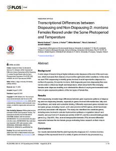
Fig 1. Map of the North Sea and its geographical position. Labels correspond to the names of specific localities in terms of areas and geographic features including banks, bights and islands mentioned in the study. https://doi.org/10.1371/journal.pone.0189731.g001

marine fish species, and have been shown to determine structure and function in marine fish communities (Table 1). Morphology of the fish species was described using body size, body shape and caudal fin shape. Life history was covered by age at maturity, while reproductive and dietary aspects were captured by, respectively, offspring size, fecundity and spawning behavior, and diet. The set of traits was selected to reflect different and complementary aspects of the ecological niche of the species, and this trait set has a high degree of resemblance to sets used in similar multi-trait studies [15,17,23,42]. Trait information was extracted from the primary literature and Fishbase [43] (S3 Table). Since trait data were not available from the North

PLOS ONE | https://doi.org/10.1371/journal.pone.0189731 December 18, 2017

4 / 19

Differences in biodiversity indicators in large marine ecosystem

Table 1. Overview of the eight selected trait categories sorted according to traits, description and ecological relevance. Trait

Trait categories

Description

Relevance

Body size

Continuous

Length a fish would reach if it was to grow indefinitely

Information on food web structure and ecological niche occupation

Age at maturity

Continuous

Age at which 50% of the individuals are sexually mature

Relates to lifespan and generation time

Fecundity

Continuous

Average number of eggs per adult female during a spawning season

Relates to energy output, allocation and production

Egg size

Continuous

Size of oocyte at spawning

Relates to spawning behavior and offspring investment

Body shape

Gadoid-like

The shape of the

Insights into predation

Flat

body

Elongated

behavior, mobility and habitat selection

Short/deep Eel-like Diet

Benthivore

Main dietary

Insights into the trophic

Piscivore

group(s)

structure of

Planktivore

communities

Bentho-piscivore Plankto-piscivore Spawning behavior

Caudal fin shape

Ob—Oviparous with benthic

Main spawning

Relates to ecological

eggs

behavior, divided

constraint on habitat selection [44]

Og–Oviparous guarders

between oviparity

Op—Oviparous with pelagic

and vivparity, and

eggs

further between the

Os–Oviparous shelterers

degree of parental

Ov—Oviparous with adhesive eggs

care, mode of release and egg

V—Viviparous

characteristics

Truncated

The shape of the

Relates to habitat

Continuous

caudal fin

selection and activity

Forked Rounded Emarginate Heterocercal https://doi.org/10.1371/journal.pone.0189731.t001

Sea for all the species, some trait data were also derived from neighboring areas (such as the Baltic Sea) or from the larger North Atlantic regions.

Biodiversity indicators Four commonly used indicators of biodiversity were calculated: species richness (SRic), species evenness (SEve), trait richness (TRic) and trait evenness (TEve). SRic was calculated as the number of unique species, while SEve was calculated as Pielou’s evenness [45]. The value of Pielou’s evenness ranges from 0 to 1, with larger values indicating a more even distribution in relative biomass among species in a sample. The trait-based biodiversity indices follow the proposed mathematical formulas suggested by [46,47], allowing for standardizing of trait values, and are calculated based on all eight traits. Both TRic and TEve are represented by a multidimensional trait space. TRic represents the multidimensional trait space occupied by the community calculated as the minimum convex hull volume which includes the trait values of all

PLOS ONE | https://doi.org/10.1371/journal.pone.0189731 December 18, 2017

5 / 19

Differences in biodiversity indicators in large marine ecosystem

species considered [47]. TRic was standardized between 0 and 1, with larger values indicating a larger convex hull volume, hence a higher richness of traits in a sample. TEve was defined as the evenness of the distribution of relative biomass of species in the trait space [9], and ranges, as in the case of SEve, from 0 to 1, depending on the degree of evenness in the distribution of biomass among traits in a sample. TRic and TEve were chosen to be comparable to their taxonomy-based equivalents, respectively SRic and SEve. The taxonomy and trait-based indicators were calculated following standard approaches implemented in the R packages “vegan” [48] and “FD” [46]. All biodiversity indicators were calculated per ICES rectangle per year and then averaged across either ICES rectangles or years to investigate temporal trends and spatial patterns, respectively. Temporal trends were assessed with generalized additive models (GAMs) [49] with a smoother function of year as the single predictor. No temporal autocorrelation was detected in the residuals. As the number of hauls conducted in each ICES rectangle per year varied from 1 to 11 (mean: 2.0, median: 2.9), all biodiversity indicators were standardized for differences in sampling size by using GAMs which effectively accounts for potential non-linear relationships. Values for each biodiversity indicator per year per ICES rectangle are reported in S2 Dataset

Natural and anthropogenic environmental drivers of biodiversity To investigate potential drivers of species and trait diversity, ten natural and anthropogenic environmental drivers were selected as covariates. The drivers were selected based on their demonstrated importance in shaping patterns of fish biodiversity in marine ecosystems [2,23,50]. Only spatial patterns of biodiversity were investigated due to two reasons: the highest variability was found across spatial scales, and not all drivers were fully available across the full temporal scale of the study. Depth was calculated by averaging the depth of sampled hauls per ICES rectangle from the NS-IBTS data. Sea bottom temperature (˚C) and sea bottom salinity data were obtained from Nu´ñez-Riboni & Akimova (2015) [51] on a monthly basis with a resolution of 0.2˚ × 0.2˚. Mean winter (Dec-Feb) sea bottom temperature and salinity were derived per ICES rectangle per year. Temperature seasonality was expressed as the difference between winter and summer (Jun-Aug) temperatures for each ICES rectangle. Salinity variability was expressed as the difference between minimum and maximum salinity within each ICES rectangle per year and then averaged across years. Phytoplankton biomass was estimated by proxy using the Phytoplankton Colour Index (PCI) [52] during quarter one and retrieved from the Continuous Plankton Recorder program provided by the Sir Alister Hardy Foundation for Ocean Science [53]. PCI is a semi-quantitative index that provides an estimate of phytoplankton biomass based on the greenness of water samples [54]. PCI data were available for the entire study period, but not for the whole study area in every year, hence spatial interpolation of this data source was performed using a GAM with a two-dimensional (latitude, longitude) tensor product smoother. Phytoplankton biomass was represented by mean quarter one PCI per ICES rectangle across all years. Seabed substrate richness and evenness were calculated based on seabed substrate classifications from The European Marine Observation and Data Network [55]. Six different substrate categories were used and substrate richness was defined as the number of categories present in each ICES rectangle. Substrate evenness was calculated as Pielou’s evenness, based on the relative coverage of substrate categories within each ICES rectangle. Anthropogenic pressure from fishing was estimated from data on the spatial distribution of international bottom trawling effort in the North Sea for two separate periods: 1990– 1995 [56] and 2003–2012 [57,58]. Beam and otter trawl effort were considered separately as recommended by Engelhard et al. [58]. Data, summary statistics and sources of environmental covariates can be found in the supplementary material (S3 Dataset and S4 Table).

PLOS ONE | https://doi.org/10.1371/journal.pone.0189731 December 18, 2017

6 / 19

Differences in biodiversity indicators in large marine ecosystem

Modelling To investigate the relative importance of natural and anthropogenic drivers in explaining the spatial patterns of biodiversity, we fitted a series of GAMs to each indicator of biodiversity. GAMs are non-parametric modelling methods that allow a high degree of flexibility in the form of the response [49]. The relationship between biodiversity indicators and drivers was only investigated for spatial patterns, as complete temporal coverage was not available for the entire study period. Two sets of GAMs were performed: one using the mean values of all natural drivers over the entire study period; and one using a reduced data set containing mean values of all natural and anthropogenic drivers for the two periods in which fishing effort data were available. All GAMs were performed with a Gaussian error term and restricted to a three degrees of freedom smoother (k = 3), equivalent to a second degree polynomial. Instead of a traditional model reduction procedure, each covariate was considered for inclusion and could reasonably be considered as having an effect, despite failing to meet an a priori determined significance level of p0.6 signifies moderate importance, while RVI