MARINE ECOLOGY PROGRESS SERIES Mar Ecol Prog Ser
Vol. 329: 23–42, 2007
Published January 11
Temporal and spatial variability of photosynthetic parameters and community respiration in Long Island Sound Nicole L. Goebel1, 2,*, James N. Kremer1 1
Department of Marine Sciences, University of Connecticut at Avery Point, Groton, Connecticut 06340, USA
2
Present address: Ocean Sciences Department, University of California, Santa Cruz, California 95062, USA
ABSTRACT: Photosynthetic parameters and community respiration were measured throughout 3 seasons at 8 stations in central and western Long Island Sound during 2002 and 2003. Light-dark bottle oxygen change was measured in a photosynthesis–irradiance (P–I) series for water from the mixed layer, and respiration was measured for surface, pycnocline, and near bottom water. P–I curves were fitted numerically to calculate biomass-specific rates of maximum photosynthesis at light saturation (P Bm), photosynthetic efficiency at low irradiance (αB) and plankton community respiration (Rc). The temporal and spatial variability of these fitted parameters, the derived parameter I k, and the concentration of phytoplankton pigments were described in relation to each other and to environmental factors. Concentrations of chlorophyll (chl) and phaeopigments (phaeo), and Rc reached maxima in summer and significantly decreased seaward along the length of the Sound. Photosynthetic parameters also reached maxima in summer, however there was no significant spatial variability. In surface waters, the average (± SD) of P Bm (1.3 ± 0.4 mmol O2 [mg chl]–1 h–1) demonstrated the lowest variability, compared to chl (6.9 ± 4.9 mg m– 3), phaeo (3.5 ± 2.5 mg m– 3), αB (10.9 ± 5.4 μmol O2 [mg chl]–1 h–1 [μE m–2 s–1]–1), I k (132.6 ± 71.9 μE m–2 s–1), and Rc (1.4 ± 0.9 mmol O2 m– 3 h–1). Chl and P Bm both varied with total daily insolation and with average irradiance of the photic zone, while P Bm was also correlated with temperature. Although P Bm and chl increased during summer, their peaks did not occur simultaneously. Temporal trends in αB were less clear-cut than for P Bm and chl, but αB was correlated with light properties of the water column. Plankton community respiration was high in surface waters and decreased with depth. Based on the relationship between Rc and chl, algal-related rates of respiration (Ra) were estimated at ~50% of total plankton community respiration. Our results do not support the common method of estimating algal respiration based on P Bm. KEY WORDS: Productivity · Primary production · Respiration · Oxygen · Chlorophyll · Phytoplankton community · Long Island Sound Resale or republication not permitted without written consent of the publisher
Autochthonous phytoplankton production has been targeted as the key contributor to hypoxia in eutrophic systems such as Long Island Sound (LIS), yet has not been well characterized in this system. Although limited investigations of the mechanisms that control hypoxia in LIS have recognized this underlying ecological process (Welsh & Eller 1991, Anderson & Taylor 2001), the scope of such studies did not allow for the characterization of rates in space and time, the estima-
tion of integrated rates for the whole Sound, or formulation of a model of primary production in LIS. As a first step for such calculations, this study reports measurements of temporal and spatial patterns in the photosynthetic characteristics and phytoplankton biomass in relation to each other and to environmental factors. Photosynthetic parameters are derived from measured variations in the phytoplankton response to light (a photosynthesis–irradiance relationship, or P–I curve; see e.g. Fig. 4). Typically, a linear response at low light levels approaches an asymptotic maximum rate at high
*Email:
[email protected]
© Inter-Research 2007 · www.int-res.com
INTRODUCTION
24
Mar Ecol Prog Ser 329: 23–42, 2007
light levels (Platt & Jassby 1976, Sakshaug et al. 1997), and high-light inhibition may or may not be observed. At least 2 photosynthetic parameters characterize the P–I response: α, the initial slope of the light curve that characterizes photosynthetic efficiency at low irradiance, and P m, the plateau of the maximum photosynthetic rate at light saturation (Platt & Sathyedranath 1993). In some instances, a third parameter β is necessary to describe photoinhibition, the reduction in productivity at higher irradiance levels (Platt et al. 1980). The version of the equation used by Walsby (1997) includes plankton community respiration (Rc). This formulation is applicable only to oxygen determinations, since the 14C method does not allow estimates of respiration (Platt & Jassby 1976, Cote & Platt 1983, Bender et al. 1987). Expressing these parameters in biomass-specific form, i.e. αB and P Bm, removes the effect of standing stock so that these physiological parameters are independent of changes in biomass. The derived parameter I k (= P Bm:αB ) evaluates where the initial slope intersects the maximum, providing a useful measure of the light level at which photosynthesis is saturated (Figueiras et al. 1994). Variation in the calculated biomass-specific photosynthetic parameters is used to characterize functional changes in the phytoplankton community, including physiological acclimation and shifts in community structure. Such variations provide quantitative insight into the effects of varying environmental conditions on specific phytoplankton production rates that are unresolved with the use of the measured volume-specific rates (Cote & Platt 1983, 1984). Characterizing P–I parameters in LIS enables synoptic estimates of the temporal and spatial variability in phytoplankton production for the first time (Goebel et al. 2006). In this paper, we characterize the temporal and spatial variability of physiological parameters of the P–I response (αB, P Bm and R c) from direct measurements of oxygen change in samples collected from central and western Long Island Sound (cwLIS) over 3 seasons during 2002 and 2003. We explore the relationships among phytoplankton metabolic rates and biomass, as well as their relationships to observed physical and chemical environmental parameters. Furthermore, we test the relationships between Rc and phytoplankton biomass or P Bm, to estimate an algal-related rate of respiration in LIS.
MATERIALS AND METHODS Site description. Long Island Sound, typically divided into western, central and eastern segments, is 160 km long and 5 to 32 km wide, with a mean depth of 21 m and a bottom depth of 30 to 60 m throughout the central and
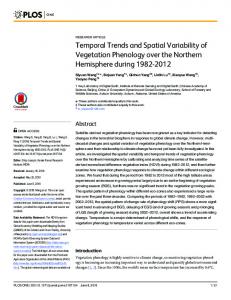
western basins. The tide is predominantly semidiurnal (Wong 1990), with an average tidal amplitude that increases 4-fold (0.7 to 2.1 m) from the eastern to the western end of the Sound (http://co-ops.nos.noaa.gov/ tides05/tab2ec2a.html#16). The turnover time for the entire Sound is 63 to 166 d (Turekian et al. 1996). Adjacent watersheds are highly populated, with more than 8 million people within the LIS drainage basin. In particular, the western end of LIS receives a large input of sewage from New York City and densely populated SW Connecticut. Salinity stratification begins during the inflow of freshwater from winter snow melt and spring rains. During the summer, physical stratification of the water column in central and western LIS (cwLIS) increases with increasing insolation and heating of surface waters (Welsh & Eller 1991, Anderson & Taylor 2001). Increased thermal stratification and relatively weak tidal and wind mixing inhibit ventilation of bottom water, leading to deteriorating oxygen levels (Welsh & Eller 1991, Torgersen et al. 1997). Stratification and increasingly hypoxic conditions are usually disrupted by storms during autumn, and occasionally during summer (Anderson & Taylor 2001). Cruise plan. We sampled 8 stations spanning cwLIS during 15 surveys of 2 to 3 d; 6 stations were uniformly distributed along the main axis of cwLIS (Stns A4, C1/C2, D3, E1, F2/F3, H4) and 2 stations were transversely distributed (Stns 9, 15) (Fig. 1). Survey cruises were biweekly during the summers of 2002 and 2003 and monthly during autumn 2002, and late spring and autumn 2003. Sampling regime. At each station, a Seabird SBE-19 SeaCat Profiler equipped with a YSI Model 5739 O2 sensor, a spherical Licor PAR (photosynthetically active radiation) sensor, underwater model 193SA, and a WET Labs WETStar fluorometer was used to vertically profile salinity, temperature, dissolved oxygen, irradiance and chlorophyll fluorescence. The profiler was mounted on a General Oceanics Model 1015 rosette system that was also used to collect water at the surface (1 to 2 m), mid-depth (within the pycnocline), and near bottom (1 to 2 m from the bottom). Discrete samples were filtered and analyzed for pigments; particulate C and N were also determined but are not reported here. Fluorometer and dissolved oxygen CTD data were calibrated with in situ water samples; these profile data were supplied by the State of Connecticut Department of Environmental Protection (CTDEP). Underwater irradiance. Attenuation coefficients (K; m–1) were calculated as the slope of the natural log of irradiance with depth (Kirk 1994). The depth of the photic zone (Zp) was defined as 1% of subsurface (0.2 m) irradiance, so that Zp _= 4.6 / K. Average irradiance within the photic zone (I zp) was calculated using the following equation (Kremer & Nixon 1978):
Goebel & Kremer: Photosynthesis and respiration in Long Island Sound
25
Fig. 1. Long Island Sound (LIS) and stations sampled. Inset: location of LIS on the NE coast of continental USA
_ Izp = I 0 (1 – e–K Zp) / (K Zp)
(1)
where I 0 is average daytime instantaneous incident irradiance (μE m–2 s–1). An analogous calculation _ was used for average irradiance in the mixed layer ( I zml) by replacing Zp with Zml in Eq. (1). Depth of the mixed layer (Zml) was determined using density profiles from the CTD casts, and defined as the depth at which density (σt) remains similar to that at the surface. Profiles of temperature, salinity and fluorescence from CTD casts were used to corroborate Zml when σt was ambiguous. When stratification was not distinct, the criterion used to distinguish a stratified from a well-mixed water column was a density difference ( σt) between bottom (maximum) and surface (minimum) waters < 0.5 kg m– 3 (Anderson & Taylor 2001). In cases of a mixed water column ( σt < 0.5 kg m– 3), Zml equaled the entire depth of the water column. Chlorophyll analysis. Triplicate samples of 250 ml from each sampled depth were filtered in the field for chlorophyll (chl) concentration through GF/F filters, transported to the laboratory on ice, and frozen until analyzed (within 2 d). Filters were extracted in 7 ml of 90% acetone overnight (18 to 20 h), mixed well, centrifuged, and read at room temperature fluorometrically before and after acidification with 2 drops of 10% HCl. The Turner Designs Model TD-700 fluorometer was calibrated with pure chl a (semiannually) and a supplied solid standard (daily). Chl and phaeopigment (phaeo) concentrations were calculated with published equations (Parsons et al. 1984). Productivity measurements. The P–I parameters were determined for rates of change of dissolved oxy-
gen (O2) in light and dark bottles. The oxygen method provides several advantages over the more commonly used 14C method in productive coastal waters. Unlike 14 C, which appears to measure something between gross and net primary production (Bender et al. 1987), measurement of the changes in O2 enables the discrimination between net and gross production. This was also tested in the present study, in a comparison of P–I curves derived from O2 and 14C methods. Although the yield of biomass under nutrient-depleted conditions may not be represented by O2-based production, we do not consider this to be an issue in the nutrient replete waters of LIS. The O2 method also enables reliable measurements of plankton community respiration, a rate unattainable with 14C. Furthermore, O2 is of fundamental interest in the study of LIS hypoxia, and direct measurements in this currency make sense. Metabolic rates were determined in 300 ml borosilicate (Pyrex) BOD bottles. Bottles were filled with an unfiltered, homogenous sample of surface water from the upper mixed layer. Each P–I series consisted of 12 light, 3 dark and 3 initial bottles. Triplicate darkincubated bottles and initial O2 concentrations were also measured on unfiltered samples from mid- and near-bottom depths. The BOD bottles were filled by overflowing with at least half a bottle volume, to avoid bubbles and air contamination. Bottles were stoppered before being placed in temperature-controlled incubators for 2 to 4 h. Dark bottles were incubated in either an incubator cooled with surface water (observed temperature range was 2.5 to 25.6°C) or an insulated box containing water from depths sampled (for pycnocline and bottom samples, the observed temperature range was 1.8 to 24.0°C). Incubation tem-
26
Mar Ecol Prog Ser 329: 23–42, 2007
peratures were maintained within 2 to 3°C of in situ temperatures. Light bottles were placed in a flowthrough incubator cooled with surface water and illuminated with an Osram Sylvania Metalarc® (metal halide) lamp. Bottles were exposed to a light gradient encompassing the irradiance range of the photic zone in LIS, from ~30 to 1500 μE m–2 s–1. Light levels were achieved by different distances from the light source, in some cases modulated with mesh screening. Light levels were measured at the midpoint of a seawaterfilled BOD bottle at each position of the incubator with a spherical PAR sensor Biospherical Instruments underwater model QSP-2100 (3.7 pi collector). Initial and incubated BOD bottles were fixed with chemical reagents for the Winkler method (manganous sulfate and alkaline iodide; Parsons et al. 1984), stoppered, sealed with water around the neck, and capped, in order to avoid contamination of samples from evaporation and air exchange around the stopper, and returned to the laboratory for subsequent analysis (within 1 wk). O2 analysis. Winkler titrations were carried out in the UCONN laboratory with a computer-controlled automatic titrator (Friederich 1991). This automated titrator analyzes the sample with a photometric detector to determine the endpoint at the wavelength of peak absorbance of the yellow iodide complex. Samples are titrated beyond the endpoint; the endpoint is determined as the intersection of linear regressions prior to and after the absorbance ceases to change with thiosulfate addition. A computer-controlled Kloehn digital pipette pump delivers increments down to 0.0005 ml thiosulfate, a precision of 0.03 mmol O2 m– 3. Replicate titrations with standards have a standard deviation of 0.06 mmol O2 m– 3 (n = 5), far better than natural variability in our replicate field samples (standard deviation of ~1 mmol O2 m– 3). P –I curve-fitting procedure. Changes in net oxygen production of the plankton community (NCP) and consumption (R c) in surface waters were normalized by average chl stock and plotted as a function of irradiance. Various equations have been used to model P–I data, resulting in substantial testing and discussion of their relative merits (Platt & Jassby 1976, Aalderink & Jovin 1997, Gilbert et al. 2000). Aalderink & Jovin (1997) and Gilbert et al. (2000) tested the variability of different model fits. Aalderink & Jovin (1997) demonstrated that the 8 models they compared could not be distinguished by their goodness of fit at the 90% level of confidence. Gilbert et al. (2000) also found that no model was superior, emphasizing that comparison of data sets should use the same model. We initially evaluated 4 models for calculated net photosynthetic rate of the community (Pc ): (Webb et al. 1974, Jassby & Platt 1976, Platt et al. 1980, Walsby 1997). The following
model was chosen from Platt et al. (1980), as modified by Walsby (1997), to include photoinhibition. I Pc = PmB ⎡⎢1 − exp ⎛⎜ − α B B ⎞⎟ ⎤⎥ − RcB + (β I ) ⎝ Pm ⎠ ⎦ ⎣
(2)
This model fit our data well and was also used by Walsby (1997) for rates of production using oxygen evolution including a chlorophyll-normalized parameter for oxygen consumption (R cB ). The interpretation of R cB is questionable, so the more meaningful Rc was fitted to Eq. (2) utilizing non-chlorophyll-specific (i.e. volumetric) oxygen change data (i.e. α and Pm). The non-linear Levenberg-Marquardt curve-fitting algorithm (FIT) and confidence interval (CONFINT) functions in Matlab® were used to fit the P –I model to our data yielding estimates with 95% confidence intervals for biomass-specific P –I parameters (αB and P Bm) and community respiration (R c ). This curve fitting procedure requires initial estimates, but no specific constraints, for the adjusted parameters. Photoinhibition was not observed and β was set equal to zero. With no necessary correction for β, the fitted P Bm represents the maximum realized instantaneous gross community production (Platt et al. 1980). Selection of P–I curves was based on goodness of fit. The criterion of adjusted r2 > 70% resulted in the removal of 10% of the P–I curves. An average coefficient of variation was calculated for the fit of each parameter to the model (Eq. 2). Comparison of R c measured directly as the average of 3 dark incubations and R c modeled with the P–I curve fitting procedure demonstrated good agreement (r2 = 0.97, p < 0.0001, n = 98), well within the standard errors of replicate BOD bottle measurements and P–I curve fits; here modeled values are used. Spectral quality. To quantify potential effects of the spectral quality of the artificial light incubator, results from the on-deck system were compared to simultaneous incubations run in situ at a central station (C1/C2 in Fig. 1). Trials on 2 dates indicated no significant differences between the calculated P–I parameters fitted on the P–I data from samples incubated on-deck versus in situ. In the first trial, αB and P Bm values and their calculated standard deviations from the fitted P–I curves of the in situ and incubated arrays were not significantly different, falling well within the range of variability observed throughout the remainder of this study. Although the parameters were also not significantly different in the second experiment, large variability in the slopes of each curve made it difficult to determine whether αB was actually not significantly different between the 2 methods. Despite the inconclusive comparison of αB in Trial 2, there were no significant effects of spectral quality on our in situ incubations based on our measurements of P Bm in both trials, and αB in the first trial.
Goebel & Kremer: Photosynthesis and respiration in Long Island Sound
Diurnal variability. Since incubations from different stations were initiated at varying times throughout the day, there was a potential bias due to diurnal variations in P–I parameters (Harding et al. 1981, 1982). Possible diurnal effects were investigated in our P–I measurements on 2 occasions during the summer of 2002. A bulk water sample (~20 l) was collected in the morning (~08:00 h), and held in large (20 l) polycarbonate bottles under subdued light for the remainder of the day. We sampled 3 overlapping P–I series and chlorophyll standing stock measurements from this reference sample throughout the daily survey (09:00 to 17:00 h). No trends in diurnal variability were observed over 2 trial experiments. One of the experiments demonstrated no significant differences among fitted P–I parameters throughout the period of the day. In the other experiment, significant differences occurred, with a minimum αB in the morning, a minimum P Bm mid-day, and a maximum P Bm in the late afternoon. These results were inconclusive and no obvious correction seems justified. In any case, seasonal, spatial and overall averages for P–I parameters were measured at a variety of initial sampling times during the photoperiod with no systematic bias. Therefore any daytime variations in productivity, which might vary with likely but uninvestigated species composition and/or environmental conditions (Harding et al. 1981), are included in the seasonal and annual variability we report. Statistics. Descriptive statistics (mean, standard deviation, coefficient of variation, range, median, quartiles and range factor (= maximum/minimum) were calculated for P–I parameters, R c, chl, phaeo, and irradiance variables measured in this study (see Tables 1 & 2). Statistical descriptors of P–I parameters and respiration exclude outliers (> 3 interquartile ranges from the edge of the interquartile range; SPSS v12.0.1). These outliers for fitted parameters are indicated in box plots that display temporal variability (see Figs. 2 & 5), but omitted from plots displaying spatial variability (see Figs. 3 & 6) and from all statistical tests. Survey-wide averages of variables in the text are reported ± SD, while fitted parameters of linear and non-linear models are reported ± SE of the estimate. ANOVA comparisons of the natural log transformations of physiological parameters (αB, P Bm, R c, and I k), _chl and phaeo, and irradiance variables (K or _ Zp, Zml, I zp, and I zml) were used to test for significant differences, indicated by p-values, in time (month and year) and space (station) (see Table 3). Although natural log transformations improved the normality of the data, Levene’s statistical test was significant across all ANOVAs, indicating heterogeneous variances. However, van Belle (2002) states that the Levene’s statistic is very sensitive to departures from the assumption of
27
homoscedasticity and should not prohibit further hypothesis testing. Therefore we proceeded with the multi-way ANOVA. In instances where there were no significant interactions within the 3-way ANOVA, we checked for significant differences among nonhomoscedasctic variables using 1-way ANOVA and the Welch and Brown-Forsyth robust tests of equality of means (SPSS v12.0.1). This secondary check reversed the significance for monthly variability in light attenuation properties (K or Zp, and Zml) only (see Table 3). With uncertainties in both variables, we applied a weighted Model II linear least squares regression, following Press et al. (1992), to estimate the average relationship between R c and chl. Log-transformation may improve the Gaussian distributions of regressed variables (e.g. Robinson & Williams 2005, p. 159), however, the log-transformed regression model did not improve the fit of our data or the normal distribution of the residuals. Regression of non-transformed variables resulted in the best model fit, and normality of the data and residuals met the assumptions of this analysis. Rates of oxygen production expressed in carbon (C) units are converted assuming a photosynthetic quotient (PQ) of 1.2. This PQ falls within the lower range of PQ for ammonium-driven production (Laws 1991). We base our estimated PQ on reports of ammonium as the primary nitrogen source for productivity in the western end of LIS (Anderson & Taylor 2001), which agrees with the direct measurements of Oviatt et al. (1986) in the waters of nearby Narragansett Bay, Rhode Island.
RESULTS Surface waters Physical environment Temporal trends. Temperature and salinity varied seasonally reaching their maxima in mid- to late-summer (Fig. 2). Surface temperatures ranged from a low of 2.5°C (May 2002) to highs in late August of 23.8°C in 2002 and 25.6°C in 2003. Variations in surface salinity lagged behind temperature, with lowest observed salinities through May (24.9) and June (23.8) of 2003 and highs in early October of 2002 (28.6) and 2003 (28.1). Interannual differences in average surface temperature throughout LIS for the 2 summers were not significant, however average surface salinity throughout LIS in the summer of 2003 was significantly lower than that in summer 2002 (p < 0.001, n = 31). Thermal stratification of the water column increased continuously during both summers, accompanied by continually decreasing bottom water oxygen concentrations
28
Mar Ecol Prog Ser 329: 23–42, 2007
Fig. 2. Spatially averaged box-plots demonstrating seasonal (temporal) variation in surface (2 m) temperature (Ts, °C) and salinity (Ss, psu), light-attenuation (K, m–1) and in_photic depth (Zp, m on right-hand ordinate), mixed-layer depth (Zml, m), average irra_ diance within photic zone and mixed layer (I zp and I zml, μE m–2 s–1), and incident irradiance averaged over each 2 to 3 d sampling period (I0, E m–2 d–1). Lower and upper lines of each box = 25th and 75th percentiles of sample, respectively; distance between top and bottom of box: interquartile range; line through middle of box: sample median (when off-center indicates skewness); vertical lines extending above and below box show extent of rest of sample minus outliers: assuming no outliers, maximum and minimum of sample are upper and lower bars across ends of vertical lines; +: outliers
(not shown). Wind and storm events disrupted the pycnocline and alleviated the hypoxic conditions of bottom waters in late September to early October of 2002 and 2003. (Trends in bottom water oxygen concentrations for these times can be seen in results of the
CTDEP hypoxia cruises at http://dep.state.ct.us/wtr/ lis/monitoring/lis_page.htm.) Significant monthly variations were apparent in light attenuation in the water column (K ), depth of the photic zone (Zp), depth of the mixing layer (Zml), aver-
29
Goebel & Kremer: Photosynthesis and respiration in Long Island Sound
2002
Ts (°C)
30
Ss (psu)
2003
20 10
Spring Summer Autumn
0 28
26
24
0.4 8 0.7
Zml (m)
3 45 30 15
IZp (µE m–2 s–1)
0 240
120
0 450 300 150 0
10
17
27
35
47
63
10
17
27
35
47
63
Distance from western end of LIS (km) Fig. 3. Mean ± SE interannual and spatial variation in surface temperature (Ts, °C) and salinity (Ss, psu), photic depth (Zp, m) and light attenuation (K, m–1, on right-hand ordinate), mixed-layer depth _(Zml, m) _and average irradiance within photic zone and mixed layer (I zp and I zml, μE m–2 s–1) averaged during summer and autumn of 2002 and spring, summer and autumn of 2003. Outliers (> 3 interquartile ranges) omitted
P–I parameters and pigments Overall trends. Fig. 4 shows 9 representative P–I curves to demonstrate and compare variability in fitted P–I parameters (αB and P Bm). These examples were
measured in the summers of 2002 and 2003 and autumn 2003 at 3 stations along the axis of cwLIS: inner (A4), mid (C1/2) and outer (H4) (Fig. 1). The P–I parameters did not vary consistently with space. Across the entire data set (minus outliers) P Bm demonstrated the lowest variability (range factor) com-
K (m–1)
Zp (m)
13
IZml (µE m–2 s–1)
age daytime irradiance _within _ the photic zone and mixing layer (I zp, I zml), and incident_ daily _ irradiance (I 0) (Fig. 2). The highest I zp, I zml and I 0 occurred during the summer of both years. A seasonal increase in K (and a decrease in Zp) was more apparent during the summer of 2002 than 2003 (Fig. 2). These descriptors of underwater irradiance (K and Zp) exhibited steep, significant along-Sound gradients (see next subsection and Fig. 3) that confounded the apparent significance of average seasonal (monthly) trends (see Table 3). During the periods sampled, incident irradiance integrated over the day (I 0; Fig. 2) ranged from the mid-summer peak in late July (60 E m–2 d–1) to a minimum in May 2003 (11 E m–2 d–1). Observed photoperiods based on local incident irradiance data (not shown) ranged from 10 h (November 2002) to 17 h (June 2003). Spatial trends. Spatial trends in temperature and salinity demonstrated small but consistent along-Sound gradients throughout the study, with lowest salinities and highest temperatures at the head (innermost western end) of the Sound (Fig. 3). These along-Sound gradients were strongest in mid-summer. Significant along-Sound gradients in K (and Zp) were also apparent throughout the study (see Table 3), with highest attenuation (0.9 to 1.0 m–1) at the innermost station during mid-summer of 2002 and early and late summer of 2003. Throughout the study, K ranged from 0.5 to 1.0 m–1 at the innermost station and 0.3 to 0.6 m–1 at the outermost station, averaging 0.6 ± 0.1 m–1 for all irradiance profiles (Table 1). Photic zone depth (Zp) averaged 8.7 ± 2.1 m for all observed irradiance profiles (Table 1) and resided within the depth of the upper mixed layer for approximately half of the observation period (average Zml = 12.0 ± 9.2 m). These values for Z p and Z ml compare well with respective ranges of 5 to 11 m and 4 to 15 m measured at Stn A4 by Anderson & Taylor (2001).
30
Mar Ecol Prog Ser 329: 23–42, 2007
Table 1. Mean, standard deviation (SD), coefficient of variation for entire data set (CV), range, median and percentiles (minimum, 25%, median, 75%, maximum), number of samples (n), and range factors (x-fold) over entire sampling duration for variables: P–I parameters (α_B, P Bm , I k = P Bm /αB), light-attenuation (K ), photic depth (Zp), mixed layer depth (Zml) and average irradiance in the _ photic zone (I zp) and mixed layer (I zml). Range factors (x-fold) are also calculated for each season. Outliers (defined as 3 interquartile ranges from edge of interquartile range) omitted from estimates of fitted parameters. See ‘Materials and methods’ for parameter units
P Bm
αB Mean SD CV Minimum 25% Median 75% Maximum n Range factor (x-fold): All Summer 2002 (n = 23) Summer 2003 (n = 30) Autumn 2002 (n = 6) Autumn 2003 (n = 13) Spring 2003 (n = 7)
10.9 5.4 0.5 2.1 7.2 10.3 14.1 29.5 91 14 5 8 10 2 4
1.3 0.4 0.3 0.3 1.0 1.2 1.4 2.5 96 5 3 3 2 2 3
Ik
K
132.6 71.9 0.5 40.7 79.9 113.2 172.5 349.2 97 9 4 5 5 2 7
0.6 0.1 0.2 0.3 0.5 0.6 0.6 1.0 98 3 3 2 1 2 2
Zp 8.7 2.1 0.2 4.2 7.4 8.4 9.6 17.2 98 4 3 2 1 2 2
Zml
_ I zp
_ I zml
12.0 9.2 0.8 2.0 6.0 9.1 15.0 44.4 98 22 7 4 5 5 6
168.6 73.0 0.4 19.5 121.2 188.1 220.0 338.8 98 17 2 12 7 2 5
178.9 144.8 0.8 17.2 67.0 126.3 272.6 682.1 98 40 9 30 4 4 11
Table 2. Statistical descriptors (as in column 1 of Table 1) for chlorophyll (chl), phaeopigments (phaeo), phaeo:chl and community respiration (Rc) at surface, mid and bottom depths. Subscripts designate surface (s), mid (m) and bottom (b) depths. Units for chl and phaeo (except for phaeo:chl) are mg m– 3, units for Rc are mmol O2 m– 3 h–1 Chls Mean SD CV Minimum 25% Median 75% Maximum n Range factor (x-fold): All Summer 2002 (n = 23) Summer 2003 (n = 30) Autumn 2002 (n = 6) Autumn 2003 (n = 13) Spring 2003 (n = 7)
Chlm Chlb Phaeos Phaeom Phaeob Phaeo:chls
Phaeo:chlm Phaeo:chlb R cs R cm R c b
6.9 4.9 0.7 2.1 3.5 5.6 7.6 24.1 98
3.0 1.6 0.5 0.5 1.9 2.9 3.7 8.7 98
1.7 1.0 0.6 0.3 0.9 1.8 2.5 4.2 98
3.5 2.5 0.7 0.9 1.9 2.7 4.6 12.4 98
2.3 1.1 0.5 0.6 1.4 2.1 2.6 5.7 98
1.9 0.9 0.5 0.3 1.3 1.6 2.5 4.8 97
0.7 0.9 1.2 0.2 0.4 0.5 0.7 6.3 98
0.9 0.6 0.7 0.3 0.5 0.7 1.3 3.0 96
1.5 1.1 0.7 0.1 0.9 1.2 1.6 6.2 96
1.4 0.9 0.6 0.1 0.7 1.4 1.9 4.0 88
0.8 0.6 0.7 0.0 0.5 0.7 1.2 2.8 76
0.7 0.5 0.7 0.0 0.3 0.6 1.0 1.9 76
11 8 8 2 3 9
19 6 19 5 2 3
14 10 11 10 3 4
14 5 14 3 3 2
9 9 4 4 2 4
15 11 8 12 2 4
27 3 27 3 4 1
10 9 9 2 3 2
56 58 6 4 4 1
28 90 10 1 16 114 2 16 7 3 12 4
60 1 33 30 4 3
pared to chl and phaeo concentrations, αB, I k and R c (Tables 1 & 2). Coefficients of variation for the averages over the entire data set were lowest for P Bm and highest for chl and Rc, with αB intermediate. The average coefficient of variation associated with the error in the fit of the P–I model (Eq. 2) for αB (0.7) was almost 3 times greater than that of P Bm (0.25). P Bm averaged 1.3 ± 0.4 mmol O2 [mg chl]–1 h–1 (equivalent to 1.0 ± 3.1 mmol C [mg chl]–1 h–1) and varied 5-fold. Chl averaged 6.9 ± 4.9 mg m– 3 and varied 11-fold. αB averaged 10.9 ± 5.4 μmol O2 [mg chl]–1 h–1 (μE m–2 s–1)–1 (equivalent to 9.1 ± 4.5 μmol C [mg chl]–1 h–1 [μE m–2 s–1]–1) and
varied 14-fold. As expected, the range factor of modelfitted parameters and environmental variables was narrower for specific seasons (Tables 1 & 2). In a multivariate ANOVA, comparisons varied significantly among sampled years (2002 vs. 2003) for αB, R c and I k, but not for chl, phaeo or P Bm (Table 3). Among summers only, ANOVA indicated significant interannual variation for αB (p < 0.001), R c (p < 0.040) and I k (p < 0.001), but not chl, phaeo, or P Bm. All P–I parameters and pigment concentrations varied significantly with month. Along the length of the Sound (by station) concentrations of chl and phaeo and rates of commu-
31
Goebel & Kremer: Photosynthesis and respiration in Long Island Sound
Table 3. A 3-way ANOVA for natural log-transformed photosynthetic parameters (α_B and P_Bm), community respiration (R c), chlorophyll (chl), phaeopigments (phaeo), I k, and irradiance variables (K and Z p, Zml, I zp and I zml) measured in surface waters along the main transect of the Sound by station (n = 8), by month (n = 8) and by year (n = 2). Significant Levene’s test (p < 0.001) rejected equality of the variances for all ANOVA tests, therefore significant differences were checked with 1-way ANOVA and Welch & Brown-Forsyth robust tests of equality of means. The only multivariate ANOVA statistics that did not hold in the 1-way ANOVA (hence deemed non-significant) were monthly variation in K and Z p and spatial variation for Zml (italicized showing both results). Values in boldface: significant at p < 0.05 level. Outliers omitted ln αB
ln P Bm
Site 0.62 Month < 0.001 Year 0.02 Site × Month 0.29 Site × Year 0.66 Month × Year 0.10 Site × Month × Year 0.29
0.08 < 0.001 0.08 0.03 0.02 0.02 0.25
Source
ln R c
ln Chl
ln Phaeo
< 0.001 < 0.001 < 0.001 < 0.001 < 0.001 < 0.001 < 0.001 0.31 0.28 0.38 0.33 0.09 0.44 0.56 0.03 < 0.01 0.41 0.16 0.28 0.50 0.10
nity respiration (R c) varied significantly. However, ANOVA tests revealed no significant spatial variability in αB, P Bm, or I k (Table 3). Temporal trends. Spatially averaged surface chl and phaeo concentrations and P–I parameters (P Bm, αB and I k) increased significantly during spring and summer seasons (Fig. 5, Table 3). Chl and phaeo concentrations peaked in late July to early August of 2002 and 2003 and in late spring (May) of 2003. (Note that our cruises did not sample December through March, thus missing a possible winter–spring bloom.) P Bm increased significantly during both summer periods, with maxima in late August of 2002 and 2003. Although monthly trends in αB were less clear-cut than in chl and P Bm, αB did peak and correlate with P Bm (r = 0.380, p < 0.001, n = 90; see later subsection) and varied significantly by month (Table 3) due to the extremes of summer maxima (June and August 2003) and an autumn minimum (November 2002). I k varied significantly throughout the observation period. A seasonal peak was more apparent during the summer of 2003; however, the maximum I k was observed in November 2002. R c increased significantly during late summer to early autumn (p < 0.0001). The maximum ratio of phaeo:chl (not shown) was detected in the following sampling period (2 wk) after the summer chl peaks. Spatial trends. Chl and phaeo decreased seaward along the length of LIS consistently during each sampling period, as demonstrated by seasonal averages (Fig. 6). During the height of each summer bloom (late July to early August), maximum chl concentrations at the head of the Sound decreased seawards 5-fold (2002) to 7-fold (2003) toward the outermost station, in central LIS. This gradient was either diminished or not evident during sampled periods of low biomass. In contrast, variability was insignificant along the Sound for biomass-specific P–I parameters (P Bm, αB, and I k) on most cruises (Fig. 6, Table 3).
ln I k 0.90 < 0.001 0.03 0.39 0.30 0.22 0.53
K & Zp < 0.001