Oct 9, 1986 - McCullough-Pitts (MP) neurons, standard artificial neural networks (ANN) . ..... Further, our research focused on the improvement of LSM and encoding a time variable. We ...... Spiking neural networks (SNN) (see Figure 6) have been called [19] the third ..... random with a bias towards "nearby" connections.
Temporal Classification and Computation Tools Inspired by Biological Neurons
Hananel Hazan
A THESIS SUBMITTED FOR THE DEGREE DOCTOR OF PHILOSOPHY
University of Haifa Faculty of Social Sciences Department of Computer Sciences
July, 2013
Temporal Classification and Computation Tools Inspired by Biological Neurons
By: Hananel Hazan
Supervised by: Prof Larry Manevitz
A THESIS SUBMITTED FOR THE DEGREE DOCTOR OF PHILOSOPHY
University of Haifa Faculty of Social Sciences Department of Computer Sciences
July, 2013
Recommended by: Professor Larry Manevitz (Advisor)
Date: 01/07/2013
Approved by: ___________________________________________ Date: _________ (Chairman of Ph.D. Committee)
I
Contents Abstract .................................................................................................................................................. IV Table of Figures ........................................................................................................................................ V 1
Introduction: ..................................................................................................................................... 1 1.1 1.2 1.3 1.4
2
What is a spatiotemporal pattern? ..................................................................................................... 1 How good are current methods? ........................................................................................................ 2 What is Temporal Computing and how can we approach it? ............................................................. 2 Why biology is a good inspiration ....................................................................................................... 3
Background and Outline of Thesis ..................................................................................................... 4 2.1 Survey of computational simulation of neurons ................................................................................. 4 2.1.1 The neuron network approach ............................................................................................... 4 2.1.2 McCullough-Pitts (MP) neurons, standard artificial neural networks (ANN) .......................... 4 2.1.3 Limitations of the ANN approach for temporal computation ................................................. 5 2.1.4 The Hodgkin-Huxley model (HH) ............................................................................................. 6 2.1.5 The Integrate and Fire (IF) neuron .......................................................................................... 6 2.1.6 Leaky Integrate and Fire (LIF) Neuron .................................................................................... 7 2.1.7 Spiking Neurons (SNNs) .......................................................................................................... 7 2.1.8 Izhikevich Neuron (IN) ............................................................................................................. 9 2.1.9 Random noise in the biological neuron .................................................................................. 9 2.2 Rate code vs. temporal code............................................................................................................. 10 2.2.1 Temporal sparse distributed memory ................................................................................... 11 2.2.2 Models of artificial neuron networks .................................................................................... 12 2.3 The Liquid State Machine (LSM): generalization and robustness ..................................................... 12
3
Results of this thesis ........................................................................................................................ 15
4
Non-Robustness of the Liquid State Machine .................................................................................. 17 4.1 Weaknesses of the basic LSM Models .............................................................................................. 17 4.2 Method and Implementation ........................................................................................................... 18 4.3 Testing Process ................................................................................................................................. 19 4.4 Variations in basic neurons: IN, MP, I&F, I&F with modifications ................................................... 20 4.5 First experiments: LSMs are not robust even for cyclic inputs ......................................................... 20 4.6 Second experiments: modifications of the LSM ............................................................................... 21 4.6.1 Different kinds of basic neurons ........................................................................................... 21 4.6.2 Allowing detectors to have memory ..................................................................................... 22 4.7 Third Experiments: changing the architecture .................................................................................. 23 4.7.1 Hub Topology ........................................................................................................................ 25 4.8 Results ............................................................................................................................................... 28 4.8.1 First experiments: LSM is not robust ..................................................................................... 28 4.9 Second experiments: varying the neurons and allowing the detectors to have memory ................ 30 4.9.1 Detectors with memory input ............................................................................................... 30 4.10 Third experiments: varying the network architecture ................................................................. 34 4.10.1 Hand chosen one-hub topology ....................................................................................... 34 4.10.2 Small world topologies ..................................................................................................... 35
II
4.10.3
Small world topologies with double power-law distribution ........................................... 37
5
Architectural conclusions ................................................................................................................ 39
6
Methodology for causing the liquid/reservoir to adapt according to input ..................................... 41 6.1 One time input test ........................................................................................................................... 41 6.2 Hebbian learning ............................................................................................................................... 41 6.3 STDP .................................................................................................................................................. 42 6.3.1 Short STDP and anti STDP ..................................................................................................... 43 6.4 Sliding threshold ............................................................................................................................... 43 6.5 Test on STDP, anti STDP and non-cyclic patterns.............................................................................. 44 6.6 Dynamic synapses and pattern recognition ...................................................................................... 47 6.7 Dynamic synapses and order based representation ......................................................................... 48 6.8 Summary ........................................................................................................................................... 49
7
Application I - Model-free hemodynamics in fMRI via reservoir computing .................................... 50 7.1 Introduction ...................................................................................................................................... 50 7.2 Brain mapping ................................................................................................................................... 51 7.2.1 Reservoir computing ............................................................................................................. 52 7.2.2 The bold signal ...................................................................................................................... 54 7.3 Methods ............................................................................................................................................ 56 7.4 Materials ........................................................................................................................................... 58 7.4.1 EXPERIMENT A. Synthetic data with varying stimulation protocols ..................................... 59 7.4.2 EXPERIMENT B. synthetic data with varying HRF shape....................................................... 61 7.4.3 EXPERIMENT C. Real dataset ................................................................................................ 63 7.5 Results ............................................................................................................................................... 64 7.5.1 Synthetic data with varying stimulation protocols ............................................................... 64 7.6 Synthetic data with varying HRF shapes ........................................................................................... 66 7.6.1 Real data ............................................................................................................................... 68 7.7 Discussion ......................................................................................................................................... 70 7.8 Software ............................................................................................................................................ 71 7.9 Appendix A ........................................................................................................................................ 71
8
Application II - Temporal pattern recognition via temporal networks of temporal neurons ............ 72 8.1 Introduction ...................................................................................................................................... 72 8.2 The Liquid State Machine.................................................................................................................. 72 8.3 Methods ............................................................................................................................................ 74 8.3.1 Liquid state configuration ..................................................................................................... 74 8.4 Data analysis ..................................................................................................................................... 76 8.5 Conclusions ....................................................................................................................................... 78
9
Future work ..................................................................................................................................... 79
10 Bibliography .................................................................................................................................... 81
III
Temporal Classification and Computation Tools Inspired From Biological Neurons Hananel Hazan
Abstract The current state of modeling artificial neurons and networks posits a significant problem of incorporating a concept of time into the machine learning infrastructure. At present the concept of time is encoded by transforming other values, such as space, color and depth. However, this approach does not seem to reflect correctly the actual functioning of biological neurons and neural networks and, moreover this leads to the exponential growth of the computing algorithm running time and of an artificially construed neural network. The aim of my doctoral thesis is to explore the concept of liquid state machines (LSM) (a neural network consisting of a large collection of units with recurrent connections) with regard to the above problem. More specifically, our aim was first to explore the correctness of the model and to identify its limitations as a model of biological neural activity; second, to improve the LSM model with regard to its identified limitations and to find another possible solution for time encoding and third, further explore the LSM concept with regard to its practical applications that until now have been very limited. By a series of experiments we were able to prove that LSM as normally defined cannot serve as models for natural neural function and that their parts are very vulnerable to failures. Our research shows that contrary to prior belief LSM are in fact not as robust (able to keep to prescribed functioning) as is necessary for their practical application. Further, our research focused on the improvement of LSM and encoding a time variable. We were able to prove that specifying certain kinds of topological constraints claimed to be reasonably plausible biologically, can restore robustness of the LSM. By adding topological constraints to the random connectivity of the network it was possible to make the network tolerant to internal damage and noise. Additionally we were able to greatly improve generalization capability of LSM by adding a sliding threshold i.e. the ability to accommodate to current input based on the history of previous input to a specific kind of neurons and learning mechanism related to spike-timing-dependent plasticity. Finally, our research focused on practical applications of LSM. Among other things, we were able to use LSM to create a model-free method of analyzing fMRI data in order to predict response of the BOLD (Blood Oxygenation Level Dependent) and to differentiate the between relevant data and noise during prediction. We were also able to use an adapted version of LSM, receiving direct real valued input, for recognition of phoneme signals in a reliable way. We learned that more reliable results are conditioned on normalizing real values of the phonemes, adding a history dependent sliding threshold to all integrate and fir neurons (LIF) in the liquid, and to topological constraints on the network connectivity.
IV
Table of Figures Figure 1: The Perceptron Model in recognition of a letter (McCullough & Pitts, 1943) ...................... 2 Figure 2: integrator .............................................................................................................................. 3 Figure 3: Coincidence detector ............................................................................................................ 3 Figure 4: McCullough-Pitts perceptrons and the classification abilities .............................................. 4 Figure 5: McCullough-Pitts (MP) Neuron. ............................................................................................ 5 Figure 6: Signal: action potential (spike) .............................................................................................. 8 Figure 7: Firing rate of a neuron ........................................................................................................... 8 Figure 8: Izhikevich neuron in action. .................................................................................................. 9 Figure 9: Model neuron response properties. (A) Response of a model neuron to a 70pA current pulse injection into the soma for 900ms. (B) Response of the same model neuron to Poisson distributed excitatory and inhibitory synaptic inputs at random locations on the dendrite. (C) Example of a back-propagating action potential in the dendrite of the model neuron as compared to the corresponding action potential in the soma (enlarged from the initial portion of the trace in B) [37]. ............................................................................................................. 10 Figure 10: Diagram of the Liquid / Echo State Machine with the input afferents and read out detectors. In our work, the elements of the liquid have been examined with different properties as has the connectivity and strength between the members of the liquid. ......... 13 Figure 11: Example of Liquid Activity, Blue Square is the slice window of the output to the readout unit. Note here the input to the readout is the activity of the liquid after the input were given to the liquid ............................................................................................................................. 19 Figure 12: Results of identification of random vectors on an untrained LSM with uniform random connections. This is a baseline. The result is a Gaussian distribution around 10 vectors. ...... 21 Figure 13: Histogram of connection distributions when the output connections were randomly selected according to a power-law. Note that the input histogram is different than the output histogram. ............................................................................................................................... 25 Figure 14: hub topology ..................................................................................................................... 26 Figure 15: Maass LSM (a) normal operation (b) with 10% dead damage (c) with 10% noise. One can easily discern the large change in the reaction of the network. ............................................. 30 Figure 16: Histographs of correctness results in LSM networks with 20 time interval input, different amounts of “dead” neuron damage, average connectivity of 20% with a uniform random distribution on the connections .............................................................................................. 33 Figure 17: Histographs of correctness results in LSM networks with 20 time interval input, different amounts of “noise generator” neuron damage, average connectivity of 20% with a uniform random distribution on the connections. ............................................................................... 33 Figure 18: Histographs of correctness results in LSM networks with one hub distribution with different amounts of “noise generator” neuron damage. ...................................................... 34 Figure 19: Histographs of correctness results in LSM networks with different amounts of “dead” neuron damage with one hub distribution. ............................................................................ 35 Figure 20: Histographs of correctness results in LSM networks with different amounts of dead neuron damage with small world topology obtained with a power law distribution. ........................ 36 Figure 21: Histographs of correctness results in LSM networks with different amounts of noise generator” neuron damage for small world topology obtained with a power-law distribution. ................................................................................................................................................ 36
V
Figure 22: Connection distribution of small-world with double power-law ..................................... 37 Figure 23: Histographs of correctness results in LSM networks with different amounts of dead neuron damage. Small world topology is obtained with a double power law distribution................ 38 Figure 24: Histographs of correctness result in LSM networks with different amounts of noise generator neuron damage for small world topology obtained with a double power-law distribution. ............................................................................................................................ 38 Figure 25: A graphical summary of the results presented in this thesis. The “standard” LSM topologies either uniform or in Maass’s original thesis are not robust; but small world topologies show an improvement, which is most marked in the case of a two-way power law distribution. ............................................................................................................................ 40 Figure 29: Liquid activity without STDP and without sliding threshold. We can see that the activity did not persist for all 1000 iteration; furthermore it’s only on a small part of the liquid. ..... 41 Figure 26: STDP rule .......................................................................................................................... 42 Figure 27: Anti - STDP rule ................................................................................................................. 42 Figure 28: Pre and Post synaptic firing. The Standard model takes into accounts all three spiking and change the weight between neuron A to B accordingly. The short model only takes into account the last spike and changes the weight according to it only. ..................................... 43 Figure 30: Liquid activity with the same parameters and input from Figure 29 but with sliding threshold and without STDP .................................................................................................. 44 Figure 33: Liquid activity with the same parameters and input as m Figure 29 but with STDP only 45 Figure 34: Liquid activity with the same parameters and the same input from Figure 29 but with STDP and sliding threshold .............................................................................................................. 46 Figure 35: Reservoir computing network. The reservoir processes a multi-dimensional input data stream x(t) generating a series of high-dimensional internal state S(t). At the same time the decoders produce the required multi-dimensional output function y(t) based on the generated internal states. ...................................................................................................... 53 Figure 36: Model used in the experiments: x(t) is an input stimuli, S(t) is an internal LSM state output, and y(t) are the synthetic BOLD signals decoded by the MLP. ............................................... 57 Figure 37: The stimulation protocol. Chunks of stimuli lasting 15-minutes are interleaved by fixation intervals lasting 3 minutes. .................................................................................................... 60 Figure 38: Snapshot of the various shapes used to generate the synthetic data with an unusual HRF. In the top plot are depicted the expected HRFs while in the bottom plot are depicted the same curves sampled at 2 seconds (as is done standardly for fMRI datasets). ............................... 62 Figure 39: Snapshot of some real voxels over a short interval of time. Two irrelevant and two correlated voxels are depicted. The vertical bars are the visual stimuli presented to the subject. The two groups of voxels are y-shifted to make the visualization more comprehensible. In fact, the absolute mean signal cannot be used to discriminate between the correlated and the irrelevant voxels. ............................................................................... 63 Figure 40: An example of a BOLD time-series on a test fold of a synthetic event related dataset. The upper graph depicts the noisy (green line), the ground truth (blue line), and the predicted (red line) BOLD signal for a relevant voxel. The lower graph depicts the same time-series for an irrelevant voxel....................................................................................................................... 66 Figure 41: t-values map for synthetic data with HRF variations determined as standard GLM analysis. Each row corresponds to one HRF variation. Columns are organized in groups of five, with
VI
increasing AR noise. The colored t-map was threshold at the highest t-value appearing in the top row (irrelevant voxels). This value was 3.07. Warm colors identify high significant t-values while cold colors identify the features with a significant but negative t-value. The grey pixels are those whose t-value has absolute value below 3.07. ....................................................... 67 Figure 42: Reconstructed BOLD time-series for a real dataset. Voxel hemodynamic response obtained with Block design, for relevant voxels (top) and irrelevant voxels (bottom). The real BOLD signal is shown in red; the generated BOLD signal is in blue. ....................................... 69 Figure 43: Diagram of the setup Liquid / Echo State Machine as used in the work. The real valued temporal signal input into the liquid, and the classifier uses the digital firing patterns of the reservoir with consecutive iteration times (synchronized to the neuron refractor period) to classify the signal. Thus each "state" in Stage 3 has a single row (liquid state) that is a snapshot of the reservoir. Hence entry to the classifier is consecutive snapshots of the reservoir's firing pattern. Eventually the final classification of the signal S(n) is done by a weighted voting between all the soft decisions over time. ............................................................................... 73 Figure 44: A general diagram of a traditional classification algorithm, where the dashed area is performed for every input window generated by the windowing procedure. If there is more than one classifier used a decision making an algorithm can be applied. .............................. 75 Figure 45: Illustration of the activity of the liquid during an input of two vectors. The first half (40bit) of both vectors are deferent patters and the second half (40bit) of both vector are the same pattern. ................................................................................................................................... 80
VII
1 Introduction: We investigate methods of developing and using spatiotemporal extensions partially inspired by biological literature) of artificial neural networks that are appropriate for classifying and simulating spatiotemporal patterns. Most applications and the classical theory of artificial neurons and networks [1] are based on the 1948 McCullough and Pitts abstraction of neurons (with slight extensions, e.g. to sigmoidal non-linearities). Since this abstraction has no time element, however, it is not surprising that these networks are more appropriate for static applications such as pattern recognition or associative memories [2] than for dynamic spatiotemporal patterns. By contrast, neurophysiologists and their modelers have long been aware of the many different and extensive temporal aspects of biological neurons (e.g. dynamic voltage, history dependent channels in neuronal gates, dynamic thresholds, and more recently dynamic synapses as well as the more classical synaptic plasticity STDP). Modelers have realized for some time that many aspects of mental processing depend precisely on these aspects; and so it makes sense to investigate their dynamic properties. In the last years, several groups [3], [4], [5], [6], [7], [8], [9] have advanced in this direction by suggesting innovative models of the Liquid State Machine (LSM) , or Reservoir Computing (RC) that uses dynamic properties of a fixed network to store spatiotemporal patterns and there was some hope that such a model could help explain human capabilities. In particular, simple examples of spatiotemporal pattern recognition like simple spoken word recognition were shown to be possible.
1.1 What is a spatiotemporal pattern? Spatiotemporal data is static data driven by time, for example: a movie consists of many static pictures that are ordered by time, and spoken words contain phonemes, vowels and consonants [10], [11] that are ordered by time. Mathematically we are interested in, e.g. classifying time series, f(t), even ones where the range of values can be complex static situations. However, mathematical representation may mislead, because one is led to treat the temporal variable similarly to the spatial variables. Mathematically, this is acceptable, but in the real world the information arrives during time and real-time solutions cannot work in this fashion. Accordingly, biological methods cannot typically do such transformations, so this detaches those methods from biological models, at least inspiration.
1
1.2 How good are current methods? Most current methods in machine learning that deal with spatiotemporal data usually work by transforming the temporal data to static space [12], for example transforming sound into an image. Then one can apply standard methods, neural networks, support vector machines and the like to the static data. However, this hugely increases the dimensionality of the data points and can result in computationally intractable situations, often called the Dimensionality Curse [13], [14] as described in [15]. That "curse" exists for a deterministic problem and multiplies many times when the problem is cast into a stochastic framework. Often, one fights this by limiting the attention to an artificial window of time as, for example [16], [17]. This can limit the information available regarding the continuity of time between windows. Moreover, the transformation of time into space for processing is quite unnatural and certainly non-biological in humans for example we always have contextual clues for events, and the windowing of the contextual clues are dynamic in size.
1.3 What is Temporal Computing and how can we approach it? How is time computed in neuroscience? In most work to date, the computational simulated neuron has been a static device in that there is no integration of signals over time (see Figure 1). As a result, the application of artificial neural networks like Optical Character Recognition (OCR), speech recognition, etc. has focused on static pattern recognition, identification and clustering. The temporal dimension is much less developed, with many applications essentially being a transformation of a temporal signal into a spatial one, with all the limitations that imposes. Most other techniques in machine learning also have this limitation [18].
Figure 1: The Perceptron Model in recognition of a letter (McCullough & Pitts, 1943)
2
Figure 2: integrator
Figure 3: Coincidence detector
Biological neurons integrate their input over time (see Figure 2), and there has been much research in the neuroscience community regarding the constants involved in this process. From the mathematical viewpoint, an abstraction of the limited “integrate and fire” neuron was pursued by [19] and their colleagues; these are also called “pulsed artificial neurons.” They have the ability to integrate and detect (see Figure 3) input signals over time, “leak,” and exemplify additional characteristics of biological neurons. Importantly, however, the constants of these simulated networks are for the most part fixed, in contrast to biological neurons, which behave more dynamically.
1.4 Why biology is a good inspiration Most information available is temporal by nature and time is part of the information needed to make decisions. Biological systems deal with this issue daily, and it has been solved quite well by nature [20], [21], [22]. For example, recognizing a song from a small sample, or the time between notes can change the tune completely. The way biological systems solve this is not completely understood, but recent development with spiking neurons can shed light on it and this approach is adopted in the present study.
3
2 Background and Outline of Thesis 2.1 Survey of computational simulation of neurons 2.1.1 The neuron network approach The basic neuronal model, published in 1943 [1], was inspired by biological neuronal principles. Since then, the models developed have been based on the same principles to do a variety of tasks. All these involve static information like handwriting, picture recognition, data categories, etc. When simulated neurons were required to deal with information with a time element, the solution required ingenuity and creativity inspiration, like the transformation of time into space or the reduction of some information in order to be able to classify the information [23], [24]. 2.1.2 McCullough-Pitts (MP) neurons, standard artificial neural networks (ANN) Artificial neural networks are by now an established technique within computer science; the first ideas and models are over fifty years old. The first generation consisted of threshold neurons. McCullough-Pitts abstracted what was thought at the time (1943) to be the properties of the neuron important for the transfer of information and computation in the brain. Their model is the basis underlying most of what are currently called “artificial neural networks.” Conceptually, it is a very simple: a neuron sends a binary ‘high’ signal if the sum of its weighted incoming signals rises above a threshold value. Although these neurons can give only a digital output, they have been successfully applied in powerful artificial neural networks like multi-layer perceptrons and Hopfield [2] nets. For example, any function with a Boolean output can be computed by a multilayer perceptron with a single hidden layer; these networks are called universal digital computations [1].
yj
wij xi
f
yi
ti : target
xi = ∑j wij yj Threshold yi = f(xi – i) yj: output from unit j Wij: weight on connection from j to i Figure 4: McCullough-Pitts perceptrons and the classification abilities
4
Note that the neuron works in lock-step; all inputs are calculated at the same time. At given fixed weights, the neuron has no “memory” of values from the previous steps. At every step, the neuron calculates from the current inputs whether to fire or not. Processing in artificial neurons typically is atemporal because the underlying basic MP neuronal model [1] is atemporal by nature. As a result, on one hand, most applications of artificial neural networks are related in some way to static pattern recognition. On the other hand, the brain science community has long recognized that the McCullough-Pitts (see Figure 5) paradigm is inadequate. Various models of differing complexity have been promulgated to explain the temporal capabilities, inter alia of natural neurons and neuronal networks.
Figure 5: McCullough-Pitts (MP) Neuron.
However, during the last decade, computational scientists have begun to pay attention to this issue from the neurocomputation perspective as well, e.g. [3], [4], [5], [25], [26], [27], [28], [29], and the computational capabilities of various models are being investigated. The basic model of a neuron consists of input weights (dendrites) toward the body of the neuron (soma); the soma does some numeric manipulation on the input weight typically summing up all inputs, and if the result passes a certain threshold it emits a spike to all the connected neurons, using the axons. 2.1.3 Limitations of the ANN approach for temporal computation The original abstraction of McCullough Pitts, based on the neuron as an adaptive logic gate, has no real time. That is, all the dendrites receive the information simultaneously; the calculation and decision of the action potential is done at a single point in time, and the neuron has no memory. (It does have memory in its architecture and “weights” but that is a different aspect.) As a result, although for static representation, clustering and learning the ANN networks have a rich developed history, for temporal information they 5
are awkward and essentially inappropriate. In contrast to natural neurons where the temporal analogues of classification are very efficient, it seems evident that an important aspect of these cells was lost in the abstraction. Despite this, the training mechanisms for such neurons are well understood and developed; although relatively less so for example, for LIF neurons (see below). The MP [1] model tries to capture the ability of a neuron to make a decision based on the input presented to it at any given moment, but the time aspect is omitted. At any given moment in time (iteration) the basic model has only the current input to compute and does not take into account the previous inputs. One step toward a simulation of a simple neuron that can represent time is the LIF neuron. Here another factor is added to the simple MP [1] model, memory, it gives the neuron the additional ability to “remember” the previous input for a certain time. 2.1.4 The Hodgkin-Huxley model (HH) A very important mathematical model that describes the electric behavior of a biological neuron is the HH Model [30]. The model is a set of nonlinear ordinary differential equations that approximates the electrical characteristics of excitable cells such as neurons and the spike activity of the entire temporal firing of a neuron via coupled differential equations, based on experiments conducted on the giant squid axon. This model explains the ionic mechanisms underlying the initiation and propagation of action potentials in the giant squid axon in biophysical mechanisms of cell current, IM, obtained from Ohm's law: Equation 1: 𝑰𝒎 = 𝑪𝒎
𝒅𝑽 𝒅𝒕
+ 𝑰𝑲 + 𝑰𝑵𝒂 + 𝑰𝑳 .
where V denotes the membrane voltage, IK is the potassium current, INa is the sodium current and IL is leakage current carried by other ions that move passively through the membrane [30]. This model has been called the “mother of computational neuroscience” because of its great success and influence. However, in this model the basic parameters do not evolve or adapt but are fixed by experimental data. 2.1.5 The Integrate and Fire (IF) neuron The HH model [30] is a numerical simulation that models the chemical and electrical properties of the neuronal cell. It is argued however that HH-type models are unable to explain action potential initiation observed in cortical neurons in vivo or in vitro [31]. Equation 2: 𝑰(𝒕) = 𝑪𝒎
𝒅𝑽𝒎 (𝒕) 𝒅𝒕
6
Moreover, the HH model requires very heavy computational resources [32]. To consider the action potential as type of communication between units (neurons) and the process of integrating inputs over time, we can simplify and describe it as a simple Integrate and Fire model [33]. The IF model described in Equation 2 is a numerical simulation of input integrated over time; when the model crosses a certain threshold it emits fire to all the connected neurons. The weakness of this model is the lack of a time-dependent memory. If the model receives an input from other neurons and did not reach the firing threshold, the signal stays the same until it fires again. 2.1.6 Leaky Integrate and Fire (LIF) Neuron To overcome the problem that the IF neurons never forget the past input, the leak is added (as showed in Equation 3) to describe the reflecting diffusion of ions that occurs through the membrane when some equilibrium is not reached in the cell. Equation 3: 𝑰(𝒕) −
𝑽𝒎 (𝒕) 𝑹𝒎
= 𝑪𝒎
𝒅𝑽𝒎(𝒕) 𝒅𝒕
2.1.7 Spiking Neurons (SNNs) Spiking neural networks (SNN) (see Figure 6) have been called [19] the third generation of neural network models, more accurately imitating the biological neuron. Besides taking into account the neuronal and synaptic state, the SNN incorporate the time concept into their operating model. The idea is that neurons in the SNN do not fire at each propagation cycle as in typical multi-layer perceptron networks, but rather fire only when a membrane potential - an intrinsic quality of the neuron related to its membrane electrical charge - reaches a specific value. When a neuron fires, it generates a signal that travels to other neurons, which in turn, increase their potentials in accordance with this signal. In the context of SNNs, current activation level is normally considered the neuron's state, with incoming spikes pushing this value higher, and either firing or decaying over time, pulling it lower. Coding methods for interpreting the outgoing spike train as a realvalue number rely either on the frequency of spikes, or on the time between them. However, recent work shows that these parameters are not fixed, but in fact are history-dependent in a seemingly complex fashion. That is, the changes are not linear with respect to recent firing-rate inputs and, in fact, are not even monotonic. This nonmonotonicity was investigated theoretically [34] and shown to arise from the reciprocal influence of chemical reactions.
7
Figure 6: Signal: action potential (spike)
Figure 7: Firing rate of a neuron
8
2.1.8 Izhikevich Neuron (IN) Izhikevich [32], [35] presents a simple, semi-empirical, model of cortical neurons, the properties of each controlled by 4 parameters. Unlike HH-type conductance-based models, the hybrid spiking models have several parameters derived from the bifurcation theory; instead of matching neuronal electrophysiology, they match neuronal dynamics.
Figure 8: Izhikevich neuron in action.
The IN is very rich in activity and very low in terms of computational load compared to most neuron simulations, especially the HH model [32]. 2.1.9 Random noise in the biological neuron A high degree of irregularity characterizes recordings of biological neuronal activity. The spike train of individual neurons is far from periodic, and the relationship of the firing patterns between neurons can be seen as a random firing (see Figure 7 and Figure 9). Whether this is indeed just noise or rather a highly efficient way of coding information cannot easily be determined. Deciding whether we are witnessing the neuronal activity underlying the composition of an electronic transmission or just meaningless noise, is a burning problem in Neuroscience [36].
9
Figure 9: Model neuron response properties. (A) Response of a model neuron to a 70pA current pulse injection into the soma for 900ms. (B) Response of the same model neuron to Poisson distributed excitatory and inhibitory synaptic inputs at random locations on the dendrite. (C) Example of a back-propagating action potential in the dendrite of the model neuron as compared to the corresponding action potential in the soma (enlarged from the initial portion of the trace in B) [37].
Not only do the neurons change and manipulate the input but the soma adds attributes to it (see Figure 9). All these factors need to be considered when creating a network simulation.
2.2 Rate code vs. temporal code Regarding computations in neural systems, the first question to ask is how information is encoded / decoded by neurons. At the present, there is no definite answer. Neuroscientists consider two kinds of codes for modeling neuron communication: rate codes and temporal codes, often confused and used interchangeably [38]. Temporal coding is considered more advanced and complex, because it assumes information is encoded in the timing of the neuronal action potentials and the precise timing of single spikes [39], while rate coding only considers the mean rate of the action potentials important [36]. For example: it is known that muscles are activated by electrical pulses (firing rate or a rate code) [39] and that motor neurons serve to convert electrical pulses generated by the brain into muscle movements, that allow animals to interact with the environment, 10
often in response to sensory stimuli they receive from it. Sensory stimuli such as light, sound, taste, smell and touch cause sensory neurons to change their activity, by firing sequences of action potentials in various temporal patterns (see Figure 7). It is hypothesized that information about the stimulus is encoded in this pattern of electrical activity. The firing rate is usually defined by a temporal average. For example, the experimentalist sets a time window of 50ms and counts the spikes in it. Division by the length of the time window gives the mean firing rate r = (number of spikes)/50ms usually reported in units of Hz. Traditionally, it has been thought that most, if not all, the relevant information was contained in the mean firing rate of the neuron, a concept successfully applied during the last 80 years. It dates back to the pioneering work of Adrian [40] who showed that the firing rate of stretch receptor neurons in muscles is related to the force applied to the muscle. Clearly, however, an approach based on a temporal average neglects all the information possibly contained in the exact timing of the spikes. It is therefore no surprise that the firing rate concept has been repeatedly criticized and is subject to ongoing debate [19], [41], [42]. In recent years, more evidence has been accumulated to suggest that a straightforward firing rate concept based on temporal averaging may be too simple to describe brain activity. One argument is that reaction times in behavioral experiments are often too short to allow slow temporal averaging. Other recent experimental results indicate that it is questionable whether biological neural systems can carry out analog computation with analog variables represented as firing rates. Due to synaptic depression the amplitude of postsynaptic potentials tends to scale like 1/f where f is the firing rate of the presynaptic neuron [33]. Therefore, both slowly and rapidly firing neurons inject roughly the same amount of current into a postsynaptic neuron during a given time window. This suggests that both a McCulloch-Pitts neuron and a sigmoid neuron model overestimate the computational capability of a biological neuron for rate codes. 2.2.1 Temporal sparse distributed memory This model [43], [44], created by Larry Manevitz, is a modification of the static associative memory of Pentti Kanerva [45]. The most pertinent for us is that it uses background noise as an implicit analogue clock, resulting in a sense of time in the associative memory. Moreover, this temporal ability comes naturally and is held to be an evolutionarily plausible mechanism. 11
2.2.2 Models of artificial neuron networks The most developed models of ANNs use the MP models as their elements. As mentioned above, it is quite successful in many ways (this is the most developed machine learning technique) [46], [47], [48], [49]. Nevertheless, some temporal properties can be obtained from such networks by examining, for example, the length of time for convergence (to attractors) [23], [24]. Meanwhile neuroscience modeling uses as a minimum the LIF neurons as the basic components since it is the simplest component having temporal properties. However, from a computational viewpoint these structures are rather complex to handle and difficult to apply in pattern matching.
2.3 The Liquid State Machine (LSM): generalization and robustness The Liquid State Machine1 (LSM) [5] (see Figure 10), has had substantial success recently. A somewhat different paradigm of computation assumes that information is stored, not in "attractors" as usually assumed in recurrent neural networks [2], [50], but in the continuing activity pattern of all the neurons that feed back in a sufficiently recurrent and interconnected network. In this way, the information is stored in a natural temporal fashion and is not transformed into spatial information. It can then be recognized by any sufficiently strong classifier such as an Adaline [46], Back-Propagation [51], Support Vector machine (SVM) [52] or Tempotron [53]. Moreover, the "persistence of the trace" (or as Maass puts it, the "fading memory" [28], [55]) allows one to recognize at a temporal distance the signal sent to the liquid and the sequence and timing effects of inputs. Fading memory in liquid state or echo state machines is the ability to retrieve memory stored in the activity patterns of the neurons for a limited period of time. As long as there is activity in the liquid or firing activity in the echo state one can retrieve the information using the detector. As time passes, however, the information or activity in the liquid or in the neurons fades or dies out, so that the activity converges to a general state hardly distinguishable from other activity patterns. At this point, the memory is degraded and cannot be retrieved. See [54], [55], [56] for a mathematically precise definition of "fading memory".
1 The name "liquid state” comes from the idea that the history of, e.g. timings of rocks thrown into a pond of water, is completely contained in the wave structure.
12
Figure 10: Diagram of the Liquid / Echo State Machine with the input afferents and read out detectors. In our work, the elements of the liquid have been examined with different properties as has the connectivity and strength between the members of the liquid.
The LSM is a recurrent neural network. In its usual format [5], [28], each neuron is a biologically inspired artificially by an IF neuron, a HH [30] or an IN style neuron [35]. The connections between neurons define the dynamic process and the recurrence connections called the topology in this thesis. The properties of the artificial neurons, together with these recurrences, result in transforming any sequence of history input into a spatiotemporal pattern activation of the liquid. The nomenclature comes from the intuitive possibility of looking at the network as a liquid like water in a pond, the stimuli are rocks thrown into the water, and the ripples on the pond are the spatiotemporal pattern. Interestingly, since the reverberations are a function of the network and its recurrency, such temporal storage is also available using static, MP neurons, for example, and this has been exploited in the Echo State machine idea. (The two situations are collectively called reservoir computing. However, see below, since the temporal aspects are solely in the network, the Echo state machine requires stronger connectivity and interneuron weights to maintain a signal, which makes it less robust than the liquid.) The use of a detector is standard in the LSM community and dates back to Maass et al [3], [28], [57], [29]. The idea is that the detectors are testing whether the information for classification resides in the liquid, and thus are not required to be biological. (How a biological network “uses” the information is a completely separate question not addressed in this model.) Thus it is theoretically possible for the detectors to recognize 13
any spatiotemporal signal fed into the liquid, so the system could be used, for instance, for speech recognition or temporal vision. In the context of LSM, the detectors are classifier systems that receive as input a state of neuronal activity (snapshot of the liquid), or in large systems, a sample of the elements of the liquid and are trained to recognize patterns that evolve from a given class of inputs. Amongst other things, it has been shown that once a detector has been sufficiently trained at any time frame, it is resilient to noise in the temporal input data and thus can be used successfully for classification; meaning that it has good generalization capabilities [25], [29], [58]. Chapter 4 describes this in more detail. Furthermore, this abstraction is said to be faithful to the potential capabilities of natural neurons and thus can be explained to some extent from the viewpoint of computational brain science. One underlying assumption is that the detector works without memory; that is, it should be able to classify from instantaneous static information; i.e. by sampling the liquid at a specific time. This is theoretically possible because the dynamic system of the liquid is sufficient to cause the divergence of the two classes in the space of activation. The detector systems such as a back propagation neural network, (BPNN) a perceptron or a support vector machine (SVM) are not required to have any biological plausibility either in their design or in their training mechanism, since the model does not try to account for the way the information is used in nature. Despite this, since natural neurons exist in a biological and hence noisy environment, for these models to succeed in this domain, they must be robust to various kinds of noise. As mentioned above, Maass et al. [28], [29], [59] addressed one dimension of this problem by showing that the systems are in fact robust to noise in the input. Thus, small random shifts in a temporal input pattern do not affect the LSM’s ability to recognize the pattern. From a machine learning perspective, it means that the model is capable of generalization. However, robustness has another component which is the liquid itself.
14
3 Results of this thesis In this thesis, we report on experiments performed with various kinds of "damage" to the LSM and unfortunately have shown that the LSM with any of the above detectors is not resistant in the sense that small damages to the LSM neurons reduce the trained classifiers dramatically, even to essentially random values [60], [61], as described in Chapter 4.1. Seeking to correct this problem, we experimented with different architectures of the liquid. The essential need of the LSM is for sufficient recurrent connections so that on the one hand, the network maintains the information in a signal, while on the other hand it separates different signals. The models typically used are random connections or those random with a bias towards "nearby" connections. Experiments with these topologies show that the network is very sensitive to damage because the recurrent nature of the system causes substantial feedback, as described in Chapter 4.7. Taking this as a clue, we tried networks with hub or small world [62], [63], [64] architecture, acclaimed [58], [65], [66] as biologically feasible. The intuition was that the hub topology integrates information from many locations and so is resilient to damage in some of them, and at the same time, since such hubs follow a power-law distribution, they are rare enough that damage usually does not affect them directly. Our experiments in fact bore out the intuition, and will be described in Chapter 4.7. With that, these methods worked well only for cyclically presented input. The more difficult case of one-time presented spatiotemporal data is found in Chapter 6.1. The approach there is to change the neurons to some whose temporal properties are historydependent. We experimented with STDP (Spike-timing-dependent plasticity) and what we call 'anti-STDP' neurons with varying success. In the end, we could produce networks robust to only certain kinds of noise so this problem is not yet completely solved. In Chapter 7 we present an application of LSMs to the problem of modelling the BOLD signal directly from data. The point is that standard BOLD signal models assume a unifying underlying model of the BOLD response. However, this is probably inaccurate especially for brain damaged patients, or, for example, those with voxels too close to a major blood vessel. We, with some colleagues, show that a completely data-driven model can be successfully developed using the LSM paradigm. We also point out that, in principle, this method could be expanded to become a new way to recognize significant voxels for a cognitive task, and could thus be used to draw brain maps. 15
In chapter 8 we present some initial developed work (joint with other colleagues) to show that the LSM methodology can be used to identify phonemes without artificial encoding in a temporal faction.
16
4 Non-Robustness of the Liquid State Machine 4.1 Weaknesses of the basic LSM Models There are two sources of potential instability. First is the issue of small variants in the input. Systems have to balance the need for separation with that of generalization. That is, on the one hand, one may need to separate inputs with small variations into separate treatment, but, with that, small variants may need to be treated as “noise” or generalization of the trained system. For the LSM, as typically presented in the literature, it is understood, e.g. from the work of [28], [57] that the LSM and its variants do this successfully in the case of spatiotemporal signals. The second issue concerns the sensitivity of the system to small changes within itself, which we choose to call damages. This is very important if, as is the case for LSM, it is supposed to explain biological systems. Our experiments, therefore, are based on simulating the LSM with temporal sequences and calculating how resistant they are to the two main kinds of damages. The damages chosen for investigation were: (1)
At each time instance, a certain percentage of neurons in the liquid would refuse to fire regardless of the internal charge in its state.
(2)
At each time instance, a certain percentage of neurons would fire regardless of the internal charge, subject only to the limitation of the refractory period.
We also checked the situation under two kinds of input schemata: 1. The neuronal reservoir gets cyclic input through the entire test while the detector tries to identify “on the fly” what pattern the reservoir “sees” at the current time. The detector identifies the pattern through the activities pattern of the reservoir. All experiments are described in Section 4. 2. The input is introduced into the reservoir only once, at the beginning of the test. After the input ceases, the detector identifies what input the reservoir received, according to the activity patterns of the reservoir. These experiments are described in section 56. Since the basic results (see Table 4 in section 4.8.1) showed that the standard variants of LSM were not robust enough to these damages at various small levels, we then considered alternatives to the basic topological connectivity of the LSM.
17
4.2 Method and Implementation To test the resistance of standard LSM to noise, we downloaded the code of Maass et al from his laboratory site2, then implemented two kinds of damage to the liquid and reimplemented the LSM code, so that we could handle variants. We simulated the liquid state machine with 243 leaky integrate and fire neurons (LIF). 20% of the neurons were inhibitory, following the exact setup of Maass and using the code available at the Maass laboratory software “A Neural Circuit Simulator”3. (To test variants of topology we reimplemented the code, available at our website4. Variants of the topologies implemented are described below as are the types of damages.) Input to the liquid was defined by inputting the identical signal to 30% of the neurons, i.e. the same input at all locations in given time instances. The detectors of these basic networks were back-propagation networks with three levels having three neurons in the hidden level and one output neuron. In most experiments, the input was given by the output of all non-input neurons of the liquid (i.e. 170 inputs to the detector). In most experiments (see Section 4 and section 56 below) the inputs to the detector were as a window of 20 sequential iterations of 170 instances and so the detector had 3400 inputs. Initially, we connected 243 units according to the topology chosen by Maass connectivity [6], [8], [28], [29], [59], [67], which prefers geometrically nearby neurons to more remote ones. Specifically, [29] regarding connectivity structure, the probability of a synaptic connection from neuron a to neuron b (as well as that of a synaptic connection 2
from neuron b to neuron a) was defined as 𝐶 ⋅ 𝑒 −(𝐷(𝑎,𝑏)/𝜆) , where λ is a parameter that controls both the average number of connections and the average distance between neurons that are synaptically connected. It was assumed that the 135 neurons were located on the integer points of a 15 x 3 x 3 column in space, where D(a,b) is the Euclidean distance between neurons a and b. Depending on whether a and b were excitatory (E) or inhibitory (I), the value of C was 0.3 (EE), 0.2 (EI), 0.4 (IE), 0.1 (II). The global connectivity of the entire network was 20%. We also did the experiment with uniform random connectivity. To test the network, 20 random patterns were generated each 80 bits in length. In some experiments, the input was entered in a cyclic fashion; i.e. the same 80 bit pattern
2
A neural Circuit SIMulator: http://www.lsm.tugraz.at/csim/
3
http://www.lsm.tugraz.at/csim/
4
http://www.cri.haifa.ac.il/neurocomputation
18
(except for generalization and error checks) repeated endlessly. In other experiments, the 80 bit pattern and its variants were entered only once commencing at time zero. All experiments were repeated 500 times, the random patterns chosen independently each time, and statistics reported.
4.3 Testing Process Initially, we experimented with two parameters: (i)
The percentage of neurons damaged.
(ii)
The kinds of damages. The kinds were either transforming a neuron into a "dead" neuron; i.e. one that never fires or transforming a neuron into a "generator" neuron, i.e. one that fires as often as its refractory period allows, regardless of its input. From the all iterations of activity the readout units received window of slices of 20 time iterations each; from the neurons designated as output neurons (see e.g. Figure 11). We tested whether the detector identified the pattern correctly at each window.
Figure 11: Example of Liquid Activity, Blue Square is the slice window of the output to the readout unit. Note here the input to the readout is the activity of the liquid after the input were given to the liquid
19
4.4 Variations in basic neurons: IN, MP, I&F, I&F with modifications We investigated the following neurons: •
Leaky Integrate and Fire (LIF).
•
LIF with sliding threshold (in two different directions; habituation to a signal and maintaining background firing rates for sensitivity).
•
Izhikevich (IN) - style neurons [35].
•
McCullough Pitts (MP) neurons [1].
With every one of the neurons above, we ran the LSM and successfully identified the training patterns without much of a problem.
4.5
First experiments: LSMs are not robust even for cyclic inputs
The experiments were as follows: for each test we randomly chose twenty temporal inputs; i.e. random sequences of 0s and 1s of length 80, corresponding to spike inputs over a period of time; and trained an LSM composed of 243 LIF neurons like those in the liquid [68] to recognize ten of these inputs and reject the other ten. Each choice of architecture was run 500 times varying the precise connections randomly. We tested the robustness of the recognition ability of the network as to the following parameters: •
The neurons in the network were either LIF neurons [57] or IN [35] neurons.
•
The average connectivity of the networks was maintained at about 20% chosen randomly in all cases although with different distributions.
•
The damages were caused by either "generators," i.e. the neurons issued a spike whenever their refractory period allowed it, or they were "dead" neurons that could not spike.
•
The degree of damage was systematically checked at 0.01%, 0.05%, 1%, 5% and 10% in randomly chosen neurons.
The results shown in tables throughout the thesis are in percentages, over the (500) repeated tests. 100% indicates that all the 20 vectors of one test, over 500 repetitions were fully recognized correctly. 50% indicates that, on average, over the 500 trials, only half the vectors were recognized. (This corresponds to a chance baseline). The graphs below show a histogram of the full distribution of all the tests and the results over all the kinds of damages and all varieties of topologies. As expected, they were distributed as Gaussian, while the average success rate varies from a baseline of 10 successes (50%) for 20
random guessing (see Figure 12) to as high as almost 20 (98%) for generalization in certain cases and 88% for some of the damages.
30 25 20 15 10 5 0 1 2
3
4
5
6
0… 9 10 11 12 13 14 0… 15 16 17 18 19 20 Success From 20 Vectors 0.01 0.03 0.05 0.07 0.09 0.1 7
8
Figure 12: Results of identification of random vectors on an untrained LSM with uniform random connections. This is a baseline. The result is a Gaussian distribution around 10 vectors.
4.6 Second experiments: modifications of the LSM 4.6.1 Different kinds of basic neurons In attempts to restore the robustness to damage, we examined the possibility that a different kind of basic neuron might result in a more resilient network. Accordingly, we implemented the LSM with various variants of LIF neurons e.g. with history dependent refractory period [34] and by using the IN model of neurons [35]. The results under these variants were qualitatively the same as the standard LIF fire neuron. (The IN model produces a much denser activity in the network and so the detector was harder to train but ultimately, the network was trainable and the results under damage were very similar.) Hence we report only results with the standard LIF neuron as appears, e.g. in Maass’ work [57]. Moreover, the tests on the LSM that use MP neurons are not reported here, because all the tests were successful, since the MP neurons do not have memory. Therefore the damages to individual neurons had a negligible effect on the stability of the whole system in every architecture tested here. 21
4.6.2 Allowing detectors to have memory In considering how to make the model more robust to damage, we investigated the fact that the detector has no memory. Perhaps if the detector was allowed to follow the network's development for a substantial time, both in training and running, it would become more robust. To check this, we took the most extreme opposite case; we assumed that the detector system in fact takes in as input a full time course of 20 iterations of the output neurons of the liquid. This means that, instead of a NN with input of 170, we had one with 20 times 170 time course inputs. It seemed reasonable that (1) with so much information, it should be relatively easy to train the detector (2) that damage in the liquid would be local enough so that over the time period, the detector could correct it. To test this, we re-implemented the LSM detector to allow for this time entry. Our detector was trained and tested as follows. There were 170 output units. At a signal point each was sampled for the next 20 iterations and all these values were used as a single data point to the detector. Thus the detector had 170 times 20 inputs. We chose separate detector points typically at intervals of 50, then used back propagation on these data points. This meant that eventually, the detector could recognize the signal at any signal points; after training there was no particular importance to the separation of the signal points except that there was no overlap between the data points. While we did not control for connections between the intervals of data points (i.e. 50, and we checked other time intervals) and possible natural oscillations in the network, we do not believe there were any. As anticipated, there was no significant trouble in training the network to even 100% of recognition of the training data. The detectors were three-level neural networks, trained by back-propagation. We also experimented with the Tempotron [53] and with a simple Adaline detector [46]. Training for classification could be successfully performed in the damage free environment with any of these. Then, we ran exhaustive tests on the possibilities. In all these tests following Maass [5], [57], [68], we assumed that approximately 20% of the neurons of the liquid were of the inhibitory type. The architecture of the neural network detector was 204 input neurons (never taken from the neurons in the LSM, also used as inputs to the LSM) 100 hidden level neurons and one neuron for the output. Results running the Maass et al. architecture are presented in Figure 15 and Table 4, and can be compared with a randomly connected network of 10% average connectivity (see Table 2). The bottom line (see section 4.8) was that even with low amount of damage inside the liquid and under most kinds of connectivity, the networks would fail; i.e. the trained 22
but damaged network loss of function was substantial and in many cases, in essence, it could not perform differently from one selected randomly.
4.7 Third Experiments: changing the architecture Our next and ultimately successful approach was to experiment with different architectures. The underlying intuition was that the recurrent nature of the liquid results in feedback of information making network dynamics that were too sensitive to internal changes. Since one can regard damages as instantaneous changes in the architecture, it seems reasonable to design architectures that can somehow filter out minor changes. Topologies of the liquids were varied in these ways: 1.
Random Connectivity. Each neuron in the network was connected to 20% of the other neurons in a random fashion.
2.
Original Maass topology. (i) Connections are chosen with a larger bias for nearby neurons [5], [57], [69]. This is the literature standard and what is usually meant by LSM. (ii) We also tested a network without such a bias; i.e. the connections to 20% of the other neurons were chosen randomly and uniformly. The results below show that these architectures are not robust.
3.
Reducing the connectivity to 10% and 5% in the above arrangement. The intuition behind this was that, with lower connectivity, the feedback should be reduced. Unfortunately, lowering the connectivity also decreases the strength the network has in representability and, importantly, in the persistence of the signal. That is, a low degree of connectivity causes the activity to die down quickly because of the lack of feedback. Thus the network is bounded in time and cannot recognize an "older" input signal. Thus as expected from the analysis in [3], [4], [5], [8], [26], [29], [59], [69], on one hand a higher connectivity gives a larger set of "filters" that separate signals, but on the other hand makes it more sensitive to changes. In any case, even with low connectivities, the random topology was not robust; nor was the Maass topology [3], [29], [69]. While not at random levels of identification, it suffered very substantial decays with even small amounts of damages. In addition, our experiments with connectivities below 15% - 20%, show that the networks do not maintain the trace for a long time. (See Table 1, Table 2, Table 5 and Table 6.)
4.
Implementation of hub topologies in either input connectivity or output. The intuition here is that the relative rarity of hubs results in their damage being very rare. When they are not damaged, they receive information from many sources and can thus filter out the damage, alleviating the feedback in the input case. In 23
the output case, the existence of many hubs should allow the individual neurons to filter out noise. Hubs were constructed in various fashions: a. Hand design of a network with one hub for input, described in full in section 4.7.1. b. Small world topologies. Since these follow power law connectivity, they produce hubs, although such topologies are thought to emerge in a natural fashion [62], [63], [64], [66] and appear in real neuronal systems [58], [62]. (See Figure 13.) However, in our context, there are two directions to measure the power law: input and output connectivity histograms for the neurons. We checked the following variants: i. Input connectivity is power law. That is, a link is assigned from a uniformly randomly chosen neuron to a second neuron chosen randomly according to a power law. In this case, the input connectivity follows a power law; while the output connectivity follows a Gaussian distribution. ii. Output connectivity is power law: the above is reversed. In this case, the input connectivity is Gaussian while the output connectivity is power law. iii. Replacing Gaussian with uniform in case (i) above. iv. Replacing Gaussian with uniform in case (ii) above. v. We also tried choosing a symmetric network with power law connectivity (i.e. for both input and output.) In this case, the same neurons served as hubs both for input and output. vi. Finally, an algorithm was designed to allow distinct input and output power law connectivity. In this case the hubs in the two directions are distinct. Algorithm 1 and Algorithm 2 below accomplish this task.
24
Liquid / Network Connectivity
Connectivity
202
11547 Inputs
11547 Outputs
152 102 52
1 13 25 37 49 61 73 85 97 109 121 133 145 157 169 181 193 205 217 229 241
2
Neurons
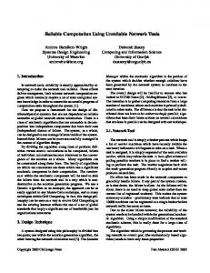
Figure 13: Histogram of connection distributions when the output connections were randomly selected according to a power-law. Note that the input histogram is different than the output histogram.
One problem with the algorithms for designing power law connectivity is that, under a "fair" sampling, the network might not be connected. This means that such a network actually has a lower effective connectivity. This problem was eliminated by randomly connecting the disconnected components, either from an input or output perspective, to another neuron chosen randomly but proportionally to the connectivity. (This does not guarantee connectivity of the graph but makes it unlikely, so that the effective connectivity is not substantially affected.)
4.7.1 Hub Topology The architecture for one hub was made as follows:
All the neurons (240) were divided into groups, the size of each randomly chosen: between 3 to 6 neurons per group. Each neuron in the group connects to 2 neighbors in the same group. A quarter of the groups were chosen to be hubs and the rest of the groups called the base. For 20% connection (that is 11,472 connections) 90% are from the base groups to the hub groups, 7% are from the hub groups back to base groups and 3% are connections between the hub groups. To accomplish that: o Random neurons are chosen (10324 times) from the base groups and randomly connected with a neuron from a hub groups. o A random neuron is chosen 803 times and connected to a randomly chosen base neuron. 25
o A hub neuron is connected 345 times randomly to anther neuron but from a different group.
Hubs
Base
Base
Base
Figure 14: hub topology
26
Algorithm 1: Generate a random number between min and max value with Power law distribution, Input: min, max, size, How_many_numbers,counterArry = array, Magnify = 5 for i = 1 to How_many_numbers index = random(array.start, array.end) end_array = array.end candidate = array[index] AddCells(array , Magnify); for t = 0 to Magnify array[end_array + t]=candidate end for shuffle(array) output_Array[i] = candidate counterArry[candidate]++ end for shuffle(counterArry) Output output_Array, counterArry Algorithm 2: Create the connectivity matrix for the liquid network using the algorithm 1 as an Input weight_Matrix use algorithm 1 to create (arraylist, counterArry) counter = 0 for i=1 to counterArry.lenght for t=1 to counterArry[i] weight_Matrix[i, arraylist[counter]]=true counter++ end for end for
27
4.8 Results 4.8.1 First experiments: LSM is not robust As there was little difference between the detectors, we eventually restricted ourselves to the back-propagation detector. (None of units of the liquid input accessed by the detectors were allowed to be input neurons of the liquid.) It turned out that while the detector is able to learn the randomly chosen test classes successfully, if there is sufficient average connectivity of 20%, almost any kind of damage caused the detector a very substantial decay in its detecting ability (See Table 3). Even with lower connectivity, which has less feedback, the same phenomenon occurs. See Table 1 (5% connectivity) and Table 2 (10% connectivity).
Table 1: 5% uniform random connectivity without memory input to the detector 5
Damage
Non
0.1%
0.5%
1%
5%
10%
Dead Neurons
100%
55%
53%
52%
51%
49%
Noisy Neurons
100%
63%
54%
55%
51%
50%
Dead & Noisy
100%
55%
52%
52%
50%
50%
Generalization
100%
93%
88%
80%
75%
78%
Table 2: 10% uniform random connectivity without memory input to the detector
5
Damage
Non
0.1%
0.5%
1%
5%
10%
Dead Neurons
100%
56%
53%
51%
51%
49%
Noisy Neurons
100%
73%
58%
54%
51%
52%
Dead & Noisy
100%
59%
54%
52%
52%
51%
Generalization
100%
100%
93%
88%
83%
81%
For all the tables that are shown in this thesis, 50% is the baseline of random classification
28
Table 3: 20% uniform random connectivity without memory input to the detector.
Damage
Non
0.1%
0.5%
1%
5%
10%
Dead Neurons
99%
60%
53%
51%
51%
50%
Noisy Neurons
99%
86%
65%
58%
52%
50%
Dead & Noisy
99%
65%
55%
53%
50%
51%
Generalization
99%
100%
97%
94%
87%
84%
When the network is connected randomly but with bias for geometric closeness as in Maass’ distribution, the network is still very sensitive, though somewhat less so. Compare Table 4 to Table 3. Table 4: 20% Connectivity under Maass’s distribution preferring local connections.
Damage
Non
0.1%
0.5%
1%
5%
10%
Dead Neurons
90%
60%
52%
51%
50%
50%
Noisy Neurons
90%
78%
57%
52%
52%
52%
Dead & Noisy
90%
54%
52%
53%
50%
50%
Generalization
90%
96%
93%
93%
84%
84%
After further experiments, we returned to this point (see concluding remarks, below). In Figure 15, the different reaction of the network is illustrated by a raster (ISI) display. With 10% damage, it is quite evident that the network diverges dramatically from the noise free situation. In Table 1 through Table 4, this is evident as well with 5% noise for purely random connectivity. Actually, with low degrees of damage the detectors, even under the Maass connectivity (See Table 4), show dramatic decay in recognition although not to the extremes of random connectivity. These results (See Table 1 through Table 4) were robust and repeatable under many trials and variants.
29
Figure 15: Maass LSM (a) normal operation (b) with 10% dead damage (c) with 10% noise. One can easily discern the large change in the reaction of the network.
Accordingly, we conclude that the LSM, either as purely defined with random connectivity, or, as implemented in [5], cannot serve as a biologically relevant model.
4.9 Second experiments: varying the neurons and allowing the detectors to have memory 4.9.1 Detectors with memory input Table 5 through Table 8 show the results with different uniform connectivity in the liquid, with memory input to the detector. Table 8 shows result similar to Table 4 for the Maass connectivity with memory input to the detector. Histographs of sample results with 5% and 10% damage for the neural network detectors are presented in Figure 16 through Figure 24 below. (Since the results for the other detectors were similar, fewer tests were carried out on them). Figure 16 through Figure 24 refer to the various kinds of hub architectures with the memory in the detector.
30
Table 5: 5% uniform random connectivity with memory input to the detector 6
Damage
Non
0.1%
0.5%
1%
5%
10%
Dead Neurons
100%
55%
53%
53%
51%
50%
Noisy Neurons
100%
63%
54%
54%
53%
51%
Dead & Noisy
100%
56%
53%
52%
51%
51%
Generalization
100%
93%
87%
80%
75%
79%
Table 6: 10% uniform random connectivity with memory input to the detector
Damage
Non
0.1%
0.5%
1%
5%
10%
Dead Neurons
100%
58%
55%
53%
49%
50%
Noisy Neurons
100%
74%
59%
57%
54%
50%
Dead & Noisy
100%
61%
54%
55%
50%
50%
Generalization
100%
96%
92%
85%
82%
82%
Architecture without memory in the detector, as presented in Table 4, can be compared with a uniform random connected network of 20% average connectivity without memory in the detector in Table 3, and as well with the Maass topology with memory in Table 8 and with uniform random of 20% connectivity with memory in Table 7. Table 1 can be also compared to Table 5 and Table 2 to Table 6. Since this thesis is about robustness, Figure 16 and Figure 17 present the full distribution of the experiments of Table 7 under these conditions with different degrees of damage. With damage over 1%, the histogram deteriorates dramatically.
6
For all the Tables that shown in this thesis, 50% is the baseline of random classification
31
Table 7: 20% uniform random connectivity with memory input to the detector
Damage
Non
0.1%
0.5%
1%
5%
10%
Dead Neurons
100%
63%
55%
52%
50%
50%
Noisy Neurons
100%
87%
67%
61%
54%
52%
Dead & Noisy
100%
68%
57%
52%
50%
49%
Generalization
100%
98%
97%
95%
89%
86%
Table 8: Maass’s distribution like in Table 4 but with memory input to the detectors.
Damage
Non
0.1%
0.5%
1%
5%
10%
Dead Neurons
100%
61%
53%
49%
49%
50%
Noisy Neurons
100%
79%
60%
55%
51%
49%
Dead & Noisy
100%
64%
55%
52%
51%
52%
Generalization
100%
100%
96%
93%
84%
85%
The bottom line of all these comparisons is that decreasing connectivity and adding memory to the detector slightly increases the robustness performance with low amounts of damage, but even so, and under all our variants of random connectivity, the networks would fail. That is, in the trained but damaged network loss of function was very substantial and, in many cases, it could not perform substantially differently from a random classification (see Figure 16 and Figure 17).
32
80 60 40 20 0 1 2
3
4
5
6
7
0… 9 10 11 12 13 14 1… 15 16 17 18 19 20 5% 1% 0.50% 0.10%
8
10%
Figure 16: Histographs of correctness results in LSM networks with 20 time interval input, different amounts of “dead” neuron damage, average connectivity of 20% with a uniform random distribution on the connections
25 20 15 10 5 0 1 2 3
4
5
6
7
8
10%
0… 9 10 11 12 13 14 1… 15 16 17 18 19 20 5% 1% 0.50% 0.10%
Figure 17: Histographs of correctness results in LSM networks with 20 time interval input, different amounts of “noise generator” neuron damage, average connectivity of 20% with a uniform random distribution on the connections.
33
4.10 Third experiments: varying the network architecture 4.10.1 Hand chosen one-hub topology Since the Maass et al. topology and the uniform random distribution topology showed a high level of vulnerability to any small amount of damage, and since adding memory to the detector helped only marginally to recover from damage in the liquid different topologies were created to test the robustness of the liquid with the same parameters as those set by Maass et al. [3], [4], [5], [6], [7], [28], [57], [69]. One of those is the hub topology described in detail in paragraph 4.7.1. In this case, Table 9, Figure 18 and Figure 19 show that robustness was substantially increased. However, under the construction as presented in paragraph 4.7.1, substantial disconnected components can appear in the liquid. Moreover, the signal has weaker persistence, i.e. detectors are able to recognize the signals only in a substantially smaller time window. Table 9: One hub network with memory input to the detector
Damage
Non
0.1%
0.5%
1%
5%
10%
Dead Neurons
100%
95%
88%
85%
76%
67%
Noisy Neurons
100%
97%
91%
86%
70%
62%
Dead & Noisy
100%
96%
89%
86%
75%
68%
Generalization
100%
100%
97%
97%
96%
95%
60 40 20 0 1 2 3 4 5 6 7 8
10%
0… 9 10 11 12 13 14 1… 15 16 17 18 19 20
5%
1%
0.50%
0.10%
Figure 18: Histographs of correctness results in LSM networks with one hub distribution with different amounts of “noise generator” neuron damage.
34
40 30 20 10 0 1 2 3 4 5 6 7
10%
8
0… 9 10 11 12 13 14 1… 15 16 17 18 19 20 5%
1%
0.50%
0.10%
Figure 19: Histographs of correctness results in LSM networks with different amounts of “dead” neuron damage with one hub distribution.
4.10.2 Small world topologies The general connectivity in the human brain has been held to have some small world properties [65]. Algorithm 1 is designed to obtain a hub topology using a more natural algorithm, creating a topology that will be robust to damage in the liquid and more natural in its construction. One property of the small world is the power-law distribution. The results of the small world with a power-law distribution (See Table 10, Figure 20 and Figure 21) were, on one hand very similar to the Maass topology and to the uniform random topology in robustness from damage in the liquid. On the other hand, they had improved generalization capability (See Table 10). Looking more closely at the distribution, as seen from Figure 13, Algorithm 1 actually creates a power-law distribution in terms of total connections, but when the connections are separated into input and output connections, it is seen that while the output has a power law distribution, the input connections have a roughly random uniform distribution. Table 10: Small World with a power-law distribution with memory input to the detector
35
Damage
Non
0.1%
0.5%
1%
5%
10%
Dead Neurons
100%
55%
51%
51%
50%
51%
Noisy Neurons
100%
79%
58%
53%
50%
51%
Dead & Noisy
100%
58%
51%
50%
48%
50%
Generalization
100%
100%
97%
93%
90%
89%
10%
5%
1%
0.50%
0.10%
25 20 15 10 5 0
1 2 3 4
5
6
7
8
0.5… 9 10 11 12 13 14 10% 15 16 17 18 19 20
Figure 20: Histographs of correctness results in LSM networks with different amounts of dead neuron damage with small world topology obtained with a power law distribution.
70 10%
60
5%
1%
0.50%
0.10%
50 40 30 20 10 0 1 2 3 4
5
6
7
8
0.5… 9 10 11 12 13 14 10% 15 16 17 18 19 20
Figure 21: Histographs of correctness results in LSM networks with different amounts of noise generator” neuron damage for small world topology obtained with a power-law distribution.
36
4.10.3 Small world topologies with double power-law distribution Accordingly, using Algorithm 1 and Algorithm 2, we created a topology with power law connectivity but it is in the reverse order for input connections and output connections as in Figure 22. For example: neuron 1 in Figure 22 has almost 250 input connections, but also two output connections, while neuron 243 in Figure 22, has almost 250 output connections, but only two input connections. In general, the two algorithms create a very specific pattern of connectivity, the number of connections to each neuron are calculated according to its neighbor by considering the input and output connectivity separately. In essence, neurons that have many output connections have less input connection and vice versa, neurons that have many of input connection have less output connections. 302
Liquid / Network Connectivity
252 12515 Inputs
152 102 52
12515 Outputs
Connectivity
202
1 12 23 34 45 56 67 78 89 100 111 122 133 144 155 166 177 188 199 210 221 232 243
2 Neurons
Figure 22: Connection distribution of small-world with double power-law
The robustness and the generalization ability was much improved, the best results were with a double-power law where the distributions are over distinct neurons. These results are presented in Table 11, Table 12 and Figure 23, Figure 24.
Table 11: Small world with a double power-law distribution with memory input to the detector
Damage
Non
0.1% 0.5%
1%
5%
10%
Dead Neurons
96%
95%
87%
83%
74%
69%
Noisy Neurons
96%
99%
93%
88%
72%
64%
Dead & Noisy
96%
97%
89%
84%
70%
66%
Generalization
96%
99%
99%
98%
97%
97% 37
Table 12: Small world with a double power-law distribution without memory input to the detector
Damage
Non
0.1%
0.5%
1%
5%
10%
Dead Neurons
62%
83%
67%
61%
56%
53%
Noisy Neurons
62%
91%
75%
66%
54%
55%
Dead & Noisy
62%
86%
69%
65%
52%
55%
Generalization
62%
100%
96%
95%
93%
91%
50 10%
40
5%
1%
0.50%
0.10%
30 20 10 0 1 2
3
4
5
6
7
8
0… 9 10 11 12 13 14 1… 15 16 17 18 19 20
Figure 23: Histographs of correctness results in LSM networks with different amounts of dead neuron damage. Small world topology is obtained with a double power law distribution.
80 60
10%
5%
1%
0.50%
0.10%
40 20
0 1 2 3 4 5 6
7
8
0.50% 9 10 11 12 13 14 10% 15 16 17 18 19 20
Figure 24: Histographs of correctness result in LSM networks with different amounts of noise generator neuron damage for small world topology obtained with a double power-law distribution.
38
5 Architectural conclusions In this work, we looked at the robustness of the LSM paradigm and by experimenting with temporal sequences showed that the basic structural set up in the literature is not robust to two kinds of damages even at low levels. We also investigated this for various degrees of connectivity. While lowering the average degree of connectivity resulted in decreased sensitivity in all architectures to some extent, the bottom line is that decreased connectivity is ineffective. In addition, it became evident that lowering the connectivity also decreases the strength the network has in representability and, importantly, in the persistence of the signal. That is, a low degree of connectivity causes the activity to die down quickly because of the lack of feedback. Thus the network is bounded in time and cannot recognize an older input signal. We see, then, as expected from the analysis [3], [5], [26], [27] that a higher connectivity gives a larger set of filters that separate signals, but on the other hand makes it more sensitive to changes. In any case, even with low connectivities, neither the random nor the Maass topology was robust. (While not at random levels of identification, as seen, e.g. in Table 2 and Table 1 it suffered very substantial decays with even small amounts of damages. In addition, other experiments not shown here, with connectivities below 15% - 20%, show that the networks do not maintain the trace for long time. ) We also investigated variants in the kinds of neurons. It seems that the LSM (or the reservoir computing concept) does not change much vis-à-vis robustness to internal noise based on these choices. There was substantial improvement when supplying a window of time input to the detector rather than an instant of time. However, this alone was not sufficient. The major effect was changing the topology of connectivity to accommodate the idea of hubs, power law and small world connectivity. Under these topologies, with the best result occurring when we have power law histograms of both input and output connectivity to the neurons, separate neurons as hubs in both directions are present, and the liquids are more robust to damages. It has been shown experimentally that the basic LSM is not robust to damages in its underlying neurons and thus without elaboration it cannot be seen as a good fit for a model for biological computation. (Data not shown here indicates that this result holds even if training is continued while the network is suffering damage.)
39
However, choosing certain power law topologies of the connectivity can result in more robust maintenance of the pertinent information over time. A graphical summary of the results for robustness under different topologies is given in Figure 25.
Liquid State Machine Framework
Liquid Topology Constraints Random Pure Random Maass biased on close neighbor
Small World Power law
Feed Forward with Hubs
Two ways power law
Figure 25: A graphical summary of the results presented in this thesis. The “standard” LSM topologies either uniform or in Maass’s original thesis are not robust; but small world topologies show an improvement, which is most marked in the case of a two-way power law distribution.
In this thesis, a distribution was chosen for biological reasons to allow preference for close neurons [58], [66]. It is superior to the totally random one, but still not sufficiently robust. Choosing a power law distribution and taking care to make different assignments for in and out connectivity proved to be the best. Since this is thought of as a potentially biological arrangement [58], [63] LSM style networks with this additional topological constraint can, as of now, be considered sufficiently biological. Other distributions may also work.
40
6 Methodology for causing the liquid/reservoir to adapt according to input 6.1 One time input test Since in the previous chapter the robustness problem for cyclic input has been solved, we now address the more difficult one of one-time input. We were only partially successful, and in the end found at this stage that we can manage robustness for damages due to dead neurons, but not to noisy neurons. For this kind of spatiotemporal signal, the goal of the model is to maintain reliable activity over time recognizing the signal at various times in spite of the dynamic damage. One difficulty with LIF, for example, is that the overall activity of the network will decay with time. Thus we found that with basic neurons, it can identify the signal immediately, but it cannot maintain reliable information over time.
Figure 26: Liquid activity without STDP and without sliding threshold. We can see that the activity did not persist for all 1000 iteration; furthermore it’s only on a small part of the liquid.
6.2 Hebbian learning Hebbian theory describes a basic learning algorithm for adjusting the connection weights in neural and artificial network models, where an increase in synaptic efficacy arises from the presynaptic cell's repeated and persistent stimulation of the postsynaptic cell. Introduced by Donald Hebb in 1949 [70], it is also called Hebb's rule: "When an axon of cell A is near enough to excite B and repeatedly or persistently takes part in firing it, 41
some growth process or metabolic change takes place in one or both cells such that A's efficiency, as one of the cells firing B, is increased" [70]. The problem with this rule is that it describes how to increase the magnitude of the connection between neurons but not how to lower the magnitude of the connections.
6.3 STDP Spike Timing Dependent Plasticity (STDP) is a biological plausible rule that is a temporally asymmetric form of Hebbian learning and also derives from experiments [71], [72]. The STDP rule is used in the learning phase when the network has received the input one time, and the synapses strengthen or weaken according to the timing of firing and the STDP rule (see Figure 27).
Figure 27: STDP rule7
Alternatively we use an anti STDP illustrated in Figure 28. The goal of the anti STDP is to decrease the effect of spikes that precede and strengthen the spikes that follow.
Figure 28: Anti - STDP rule8
Each neuron increases or decreases the weight of the connection between the preand post-synaptic neuron according to the length of time it fires. If the post-neuron fires,
7
The figure taken from [73]
8
The figure is modified from Figure 27: STDP rule[73]
42
it checks how close it is to pre-synaptic firing, and increases the weights' magnitude in proportion to the time elapsed (i.e. a neuron that fires relatively close to the pre-synaptic firing receives more weight than a synapse that transferred a spike a long time ago but still within the window time frame of change). If the post-neuron fires after the preneuron fired, the pre-neuron decreases the weight between the post-neuron to itself in relation to the time of firing (i.e. neuron that fires right after decreases more than one that fires long afterwards, but still in the time frame of change). 6.3.1 Short STDP and anti STDP The difference between the standard STDP and the short STDP is that the standard model takes all history of firing from each neuron and changes the weights accordingly. The short version only takes into account the last firing from the pre-synaptic neuron. See Figure 29: the short STDP accounts for only the third and last fire from neurons A to B and calculates the change of weight accounting to this timing of the last firing, while the standard STDP model does so for all the three firing timings and changes the weight according to the sum of all three. Spikes Neuron A
Pre Synaptic
Post Synaptic
Neuron B Figure 29: Pre and Post synaptic firing. The Standard model takes into accounts all three spiking and change the weight between neuron A to B accordingly. The short model only takes into account the last spike and changes the weight according to it only.
6.4 Sliding threshold The problem addressed was that the neurons in the liquid do not regulate their activity and, as seen in Figure 26, the activity dies out quickly once input ceases. The sliding threshold [73] habituates the firing, making the neuron harder to fire once it is functioning at about 80% of its maximal firing capacity. At initialization, each neuron from the network has its constant decay rate set randomly between 0 to 1. If the neuron does not receive input from another neuron or from an external source, the neuron reduces its threshold by a constant rate, until the neuron receives input or the threshold equals the resting voltage. After a spike the neuron resets to the initial threshold. 43
Figure 30: Liquid activity with the same parameters and input from Figure 26 but with sliding threshold and without STDP
If the neuron receives inputs that cause it to spike more than 80% of its maximum capability, the neuron increases its threshold by the constant rate until its firing rate is lower than 80% of its capability. In addition, the sliding threshold is adjusted in the other direction thus making the neuron more sensitive to firing when the rate of spikes reaching it is very low. See Figure 26, compare with Figure 30. The sliding threshold problem is that it makes the neurons much more sensitive to noise in the liquid itself or in the input to the liquid. The results are random (about 50% recognition) in almost all cases of even small noise. Hence another method was needed to strengthen the relevant and important connections between the neurons. That is why we additionally used the STDP rule (see above).
6.5 Test on STDP, anti STDP and non-cyclic patterns To enable the liquid to handle the non-cyclic input, before modifying the readout neurons on the signal, we first created a study phase. There the network received the input once (as in the testing phase) but during that phase the synapses were allowed to change according to the STDP rule (see Figure 27).
44
We also used a different STDP illustrated in Figure 27 and Figure 28. The purpose of this variant anti-STDP is to perform the standard STDP effect of spikes that precedes and weakens the spikes that follow.
Figure 31: Liquid activity with the same parameters and input as m Figure 26 but with STDP only
Secondly, both rules decrease the effect of pre-synaptic neurons that fire after the post-synaptic firing, again in relation to the time of firing. For STDP the effect of a presynaptic neuron that fires slightly after a post-synaptic firing neuron decreases under STDP more than one that fires a long time before that firing, but still in the window time frame of change whereas for anti STDP this is reversed. Here as in Figure 31, the result of activity due to using a liquid with only STDP and without the sliding threshold is a long activation of the liquid. With that the activation is not easily separable for classification or it is very hard to separate, because it is monotonic and repeated throughout the time period. Figure 32 shows the result of using the best arrangement with the same one as Figure 26 but with both the sliding threshold and the STDP.
45
Figure 32: Liquid activity with the same parameters and the same input from Figure 26 but with STDP and sliding threshold
Table 13 and Table 14 show the final results of this thesis using both STDP and the sliding threshold. Dead Neurons damage Recognition Ability Versus Topology Topology Variability / Differences 1% 3% 5% 7% 10% Random 0.80 0.74 0.72 0.69 0.66 Directional style network 0.87 0.76 0.72 0.66 0.64 Maass 0.83 0.74 0.72 0.70 0.66 Small worlds 0.82 0.74 0.71 0.68 0.65 Table 13: Result on non-cyclic input with standard STDP and sliding threshold
Damage on the input – Generalization recognition Generalization Recognition Ability Versus Topology Topology Variability / Differences 1% 3% 5% 7% 10% Random 0.92 0.87 0.84 0.85 0.86 Directional style network 0.94 0.89 0.89 0.89 0.88 Maass 0.92 0.86 0.86 0.84 0.85 Small worlds 0.93 0.87 0.85 0.80 0.82 Table 14: Result on non-cyclic input with standard STDP and sliding threshold
46
With the same setup as the above but with the Anti STDP, we found that the network has very poor fault tolerance (Table 15) and poor generalization abilities (Table 16.)
Noise damage Recognition Ability Versus Topology Topology Variability / Differences 1% 3% 5% 7% 10% Random 0.53 0.54 0.53 0.5 0.51 Directional style network 0.51 0.52 0.51 0.5 0.5 Maass 0.51 0.51 0.53 0.52 0.52 Small worlds 0.51 0.53 0.51 0.51 0.52 Table 15: Liquid performance on non-cyclic input with Anti STDP and sliding threshold
Input generalization recognition Generalization Recognition Ability Versus Topology Topology Variability / Differences 1% 3% 5% 7% 10% Random 0.7 0.58 0.57 0.58 0.61 Directional style network 0.79 0.72 0.68 0.7 0.71 Maass 0.74 0.63 0.61 0.62 0.63 Small worlds 0.72 0.6 0.61 0.61 0.62 Table 16: Liquid performance on non-cyclic input with Anti STDP and sliding threshold
6.6 Dynamic synapses and pattern recognition Following the work of Shahaf [74], we questioned whether the ideas presented above would persist when the network has dynamic synapses. It was tested only for the simplest case where synapses become unavailable after frequent firing for a set period of time. Somewhat surprising, the system retained its resilience to noise and its generalization ability as long as we used both the sliding threshold and the STDP properties. However, the training time for STDP had to be multiplied by five.
47
Dead Neurons damage Generalization Recognition Ability Versus Topology Topology Variability / Differences 1% 3% 5% 7% 10% Random 0.82 0.76 0.70 0.70 0.66 Directional style network 0.85 0.76 0.71 0.69 0.64 Maass 0.85 0.75 0.69 0.66 0.67 Small worlds 0.80 0.73 0.66 0.65 0.64 Table 17: Dynamic Synapses. Results for non-cyclic input with standard STDP and sliding threshold
Damage on the input – generalization recognition Generalization Recognition Ability Versus Topology Topology Variability / Differences 1% 3% 5% 7% 10% Random 0.92 0.85 0.86 0.83 0.84 Directional style network 0.94 0.87 0.88 0.85 0.88 Maass 0.91 0.86 0.84 0.85 0.84 Small worlds 0.90 0.82 0.81 0.79 0.79 Table 18: Dynamic Synapses. Results for non-cyclic input with standard STDP and sliding threshold
6.7 Dynamic synapses and order based representation A main insight of Marom et al [74] was that, under natural biological networks, order based pattern encoding is sufficient for pattern identification and, it is claimed, an emergent property of the system. We made the same attempt for our best system and did in fact show that this works both for static and dynamic synapses: Table 19 and Table 20 show the result for static synapses networks and Table 21 and Table 22 for dynamic synapses. These results, then, help support the claims of Shahaf [74].
Dead neurons damage Recognition Ability Versus Topology Topology Variability / Differences 1% 3% 5% 7% 10% Random 0.68 0.64 0.61 0.59 0.57 Directional style network 0.73 0.62 0.58 0.57 0.55 Maass 0.67 0.62 0.57 0.59 0.56 Small worlds 0.65 0.61 0.60 0.57 0.55 Table 19: Result on non-cyclic input with standard STDP and sliding threshold with static synapses
48
Damage on the input – Generalization recognition Generalization Recognition Ability Versus Topology Topology Variability / Differences 1% 3% 5% 7% 10% Random 0.83 0.73 0.7 0.72 0.66 Directional style network 0.83 0.78 0.7 0.73 0.69 Maass 0.83 0.74 0.71 0.71 0.69 Small worlds 0.84 0.74 0.68 0.68 0.69 Table 20: Result on non-cyclic input with standard STDP and sliding threshold with static synapses
Dead neurons damage Recognition Ability Versus Topology Topology Variability / Differences 1% 3% 5% 7% 10% Random 0.67 0.65 0.59 0.59 0.56 Directional style network 0.67 0.63 0.60 0.55 0.56 Maass 0.67 0.64 0.59 0.58 0.57 Small worlds 0.66 0.62 0.59 0.56 0.55 Table 21: Result on non-cyclic input with standard STDP and sliding threshold with dynamic synapses
Damage on the input – generalization recognition Generalization Recognition Ability Versus Topology Topology Variability / Differences 1% 3% 5% 7% 10% Random 0.84 0.74 0.70 0.71 0.69 Directional style network 0.83 0.75 0.74 0.72 0.75 Maass 0.84 0.75 0.71 0.70 0.72 Small worlds 0.81 0.73 0.68 0.68 0.64 Table 22: Result on non-cyclic input with standard STDP and sliding threshold with dynamic synapses
6.8 Summary We have investigated the LSM under variations designed to make the system applicable for spatiotemporal pattern identification both under cyclic and non-cyclic input. It was discovered that this can be done with the choice of a directional topology, and a sliding threshold and learning method applied to the connections in the liquid. 49
7 Application I - Model-free hemodynamics in fMRI via reservoir computing Standard methods for the analysis of functional MRI data rely strongly on prior implicit and explicit hypotheses made to simplify the analysis. In this work the attention is concentrated on two such commonly accepted hypotheses: (i) the hemodynamic response function to be searched in the Blood Oxygenation Level Dependent (BOLD) signal is typically described by a specific parametric model e.g., double-gamma; (ii) the effect of stimuli on the signal are taken to be linearly additive. While these assumptions have been empirically proven to generate high sensitivity for statistical methods, they also limit the identification of voxels relevant to what is already postulated in the signal, thus blocking the discovery of uncommon or novel knowledge. We tried to overcome these limitations by a model-free approach to fMRI data analysis, where in the BOLD response is learned directly from data rather than assumed in advance. As a result, this approach produces a set of voxel-wise models of the “real” BOLD response, meaning that relevant voxels are filterable according to their prediction accuracy in a machine learning framework. We present here a computational architecture based on the paradigm of reservoir computing wherein a LSM is combined with a decoding feed-forward neural network. An empirical analysis on synthetic data sets shows that the learning process can be robust both to noise and to the varying shape of the hemodynamic response function. A similar investigation on real fMRI data sets provides evidence that BOLD predictability allows for discrimination between relevant and irrelevant voxels for a given set of stimuli.
7.1 Introduction Functional Magnetic Resonance Imaging (fMRI) is a widely used modality in studies of brain perception and cognition, applying to a broad variety of neuroscientific questions including brain mapping, which corresponds to the set of data analysis methods designed to detect and map brain areas relevant to specific cognitive or perceptual tasks. The fMRI experiments are usually designed by contrasting categories of stimuli, e.g., visual representation of faces versus houses, and analyzing the recorded data to find brain areas related to classes of stimuli. The underlying assumption is that the brain areas allowing discrimination between contrasting categories are related to the corresponding cognitive or perceptual task. Existing brain mapping methods can be divided into hypothesis-driven and datadriven methods. The former use various prior assumptions regarding the basic characteristics of BOLD signal, while the latter class of methods, usually exploratory in 50
nature, tries to infer these characteristics directly from fMRI data. The present work, belonging to the second category, introduces a data-driven approach to BOLD response analysis using Reservoir Computing, a machine learning technique explicitly designed for complex temporal signal processing [9], [29], [61]. With it, we implemented a supervised learning schema that predicts the BOLD signal in response to a sequence of stimuli in input. A training process is required for each voxel and for each set of stimuli. The success of this trained predictor on test data indicates the voxel's relevance for the perceptual/cognitive task. Potentially, the proposed method allows for the discovery of unknown functional dependencies between the BOLD signal and the known set of stimuli with a completely model-free data-driven approach that makes no prior assumption regarding the expected hemodynamic function.
7.2 Brain mapping Hypothesis-driven methods for the fMRI data analysis are used in most brain mapping studies. Indeed, a recent survey [75] of 170 fMRI studies shows that 96% of experiments were based on the hypothesis-driven analysis methods. These methods have a strong statistical framework for assessing the relevant regional activation areas. However, they rely on prior assumptions as to the BOLD signal underlying the real brain activity. Given a stimulation protocol, prior knowledge makes it possible to define the expected BOLD response as a parametric hemodynamics response function (HRF), used in a general linear model (GLM) framework [76], resulting in a univariate analysis of the correlation between the real signal and the estimated HRF. These methods require, therefore, an accurate definition of the expected HRF shape, although it may vary significantly in different populations between subjects and between different brain areas [77]. Recent sophisticated HRF models attempt better to capture the complex structure of the BOLD response [78]. Nonetheless, these parametric models still encode the ideal BOLD shape without allowing for possible confounds in the design protocol and without including the dependencies due both to the brain structure (e.g., proximity to a large vascular vessel or changes caused by different brain injuries) and to the cognitive/perceptual tasks under investigation. To avoid these issues, one can try to obtain a correct HRF voxel by voxel with a data-driven approach, thereby finding the unknown functional dependencies between the BOLD signal and the known set of stimuli, without any prior assumption as to the expected HRF. Some data-driven methods are reported in the literature, such as selective averaging with a long inter-stimulus interval assuming non-overlapping responses [79]. Trials with overlapping responses are also averaged, ignoring that the overlaps introduce errors. 51
Other methods, like Bayesian approaches [80] or wavelet deconvolution [81] are computationally expensive or require additional prior assumptions like separability of signal and noise in the frequency domain for the wavelet methods. Alternatively, Wang [82] proposed a data-driven method based on machine learning techniques. It combines the HRF data-driven analysis with the hypothesis-driven GLM inference about the relations between the given design matrix and the recorded BOLD signal. In this method, the HRF profile extracted from the support vector machine (SVM) classifier [83], [84] is used as the data-driven regressor for the consequent GLM analysis (SVM is a machine learning technique with demonstrated success in the analysis of neuroimaging data in many applications [85], [86], [87], [88], including particular brain-decoding, an approach that contrary to standard brain-mapping analysis tries to predict the contrasted stimuli from the existing BOLD signal). By contrast, the HRF derivation discussed here is a reverse task in which we wish to reconstruct the expected BOLD signal shape based on the stimuli sequence. Significantly, the substantially temporal nature of both BOLD signal and the designed stimuli sequences make it difficult to use the SVM based methods efficiently without complex preprocessing procedures encoding the temporal data dimension into a spatial one. Such an encoding scheme is also subject to limitations in terms of the total experiment length. Furthermore, the prior assumption on the length of the constant temporal data profile between different repetitions needs to be verified to make the results of this method valid [82]. 7.2.1 Reservoir computing In the current study we addressed the HRF decoding task without encountering the above temporal issue, and using a method based on reservoir computing. Its main principles can be explained through analogy with a pebble thrown to a pond. When a small pebble is thrown to a pond full of water (a liquid reservoir), it generates waves representing a series of liquid states that can be measured at different time steps. Each liquid state represents a unique trace of the past activity. This way, the liquid reservoir’s latest state contains the history of all previous events, enabling the efficient encoding of temporal information. That series of consequent states can be recorded with any suitable device and further exploited/analyzed. The device responsible for “reading” or “decoding” the information from the internal reservoir states is called a readout, or decoder. The readout typically identifies the desired series of events based on the internal reservoir states. The decoder can produce a required series of signals functionally related to the input [69]. More specifically, a reservoir system (Figure 33) is made of two components: (i) the reservoir, a nonlinear dynamical system based on a recurrently coupled network of 52
artificial neural computational nodes; (ii) a sufficiently strong decoder or readout retrieving the temporal information in the reservoir’s states and producing the desired output time-series. The reservoir is used to encode a nonlinear transformation of the input stream, capturing the past history into a high-dimensional reverberating internal activity state. From a machine learning perspective, a reservoir operates as a temporal kernel, projecting the input to a dynamic nonlinear high-dimensional space. The reservoir states form a trajectory dependent on both the current external input and the memory traces of previous stimuli. In this way, reservoir architectures can inherently process spatiotemporal patterns. The power of this system is based on the separation between the network layer functions: the reservoir expands the input history into a rich state space, while the decoder combines the series of the internal states into the desired output signal.
Figure 33: Reservoir computing network. The reservoir processes a multi-dimensional input data stream x(t) generating a series of high-dimensional internal state S(t). At the same time the decoders produce the required multi-dimensional output function y(t) based on the generated internal states.
The computations of the reservoir computer are driven by the underlying recurrent neural network dynamics and may be expressed as: Equation 4: {
𝑺(𝒕)
=
𝑳(𝒙(𝒕), 𝑺(𝒕 − 𝟏))
𝒚(𝒕)
=
𝑫(𝑺(𝒕))
where the internal network state S at time t is generated by an operator L integrating the input value x to the network at current time t with the previous internal network state at time t-1. This transformation creates a new high-dimensional reservoir activity pattern carrying the information about the entire input sequence. The exact definition of L depends on the type of neurons and the topology used to construct the network. Based on a newly generated internal state S(t), a memory-less decoder function D transforms the current liquid state into the machine output (t). The detector function D is commonly 53
implemented using a classification or a regression algorithm trained with simple learning mechanisms. The whole architecture is designed to make the learning as fast and robust as possible [89, pp. 275–296]. It delegates the primary load of the goal-directed learning to a single and seemingly trivial output stage, which typically is a relatively simple computational component. The reservoir serves as pre-processor for such a detector unit, creating the range of possible projection functions of the input streams x(t) that the detector can learn. Such division of computational processing into reservoir and decoder is efficient since the same reservoir can serve a large number of decoders trained to extract different information from the same internal state sequence. As described above, there is a certain similarity between reservoir and kernel methods. The reservoir can be seen as a nonlinear transformer of temporal information into a higher-dimensional space. There are however significant differences between the two methods. In the case of reservoirs, mapping into the new space is explicitly temporal. In addition, reservoir computing manages both inputs and outputs as streams of data potentially in continuous time [89], [90]. The temporal dimension makes this model particularly suitable for fMRI data analysis, with both input stimuli and output BOLD signals representing relatively long data streams. 7.2.2 The bold signal The whole brain BOLD activity may be modeled by as many functions as the number of voxels. For each voxel i its BOLD signal i(t) at time t, as recorded by an fMRI scan, is described by an unknown function fi(t), which encodes the dependency of the voxel behavior from the entire sequence of stimuli: Equation 5: 𝒚𝒊 (𝒕) = 𝒇𝒊 (𝒙[𝒕𝟎; 𝒕] ) + 𝜺𝒊 (𝒕)
where 𝑥 [𝑡0;𝑡] = [𝑥(𝑡0 ); … ; 𝑥(𝑡)] is the stimuli time-series from the beginning of the experiment to the current time step t, and 𝜀𝑖 (𝑡) is an unknown function describing the noise and any unknown component of the BOLD signal not related to the external stimuli. If the voxel behavior has relationships with the sequence of stimuli the function fi (t) in Equation 5 is not null. On the contrary, if the voxel is not influenced by the external stimuli, the function fi (t) is a null component and the entire signal is described by 𝜀𝑖 (𝑡). The formalization describes a non-Markovian process, where the BOLD activity may, in principle, depend on the entire past sequence of stimuli, although it is commonly assumed that the hemodynamic response takes less than 20 seconds to recover to the initial state. The function fi (t) may be implemented by a Markovian representation as: 54
Equation 6: 𝑴(, 𝐢 ) = {
𝑺(𝒕) = 𝒉 (𝑺(𝒕 − 𝟏), 𝒙(𝒕)) 𝒚𝒊 (𝒕) = 𝒈𝒊 (𝑺(𝒕)) + 𝜺𝒊 (𝒕)
where the output function 𝑔𝑖 replacing fi (t) is now based on an internal state S only, determined by a transition function ℎ , which encodes the entire input history as a function of the previous state and the current stimulus. The transition and the output functions ℎ and 𝑔𝑖 are instantiated by the parameters and respectively. The parameter for the transition function ℎ and the state S are common to all voxels, while the parameters for the output functions 𝑔 are different for each individual voxel. For the system 𝑀(, 𝑖 ) to be Markovian, the transition function ℎ must preserve all the past information in x(t-1). However, since time-series in neuroscience experiments are not infinite, we may implement ℎ with a finite memory dynamic system. In particular, the system described in Equation 6 may be implemented using the reservoir computer defined by Equation 4. In this mapping, the input signal x(t) describes the stimuli sequence used in the experiment, the reservoir states S(t) represent internal neural activity caused by the stimuli, and, finally, the decoder output y(t) characterizes the model of the oxygenation producing the BOLD signal relevant for a given activity pattern. Functions ℎ and 𝑔𝑖 may be substituted by the reservoir operator L and the decoder function D respectively. The reservoir plays a central role in the proposed system by representing the temporal dimension of the presented stimuli sequence in its state. Moreover, thanks to its fading-out property in the absence of external input, it may forget the preceding series of internal states/inputs imitating the final nature of basic BOLD response where all blood parameters return back to the bases level in the absence of a new stimulus. The operational cycle of a reservoir computer as applied to the analysis of BOLD signal is depicted in Figure 33. The binary stimuli vector 𝑥(𝑡) describing the time series of impulse-like stimuli 𝑥(𝑡) = [𝑥1 (𝑡), … , 𝑥𝑚 (𝑡)]T (where m is a number of different classes of stimuli used in the experiment) is provided as input to the reservoir without any additional pre-processing steps. It is fed into the reservoir network, value by value, a step at a time. The reservoir integrates the information in a parallel computation and produces a series of rich high-dimensional internal activity states 𝑆(𝑡) encoding all past input. At the same time, the decoder units D1…Dn (where n is a number of voxels in the brain) recreate the BOLD signal 𝑦1 (𝑡) … 𝑦𝑖 (𝑡) based on the encoded internal state. Using information metrics (e.g. correlation or mean squared error), it is therefore possible to evaluate the similarity between the voxel BOLD signal reconstructed by the reservoir computer and the real BOLD signal detected by fMRI scanner, both generated in response to the same stimuli sequence. 55
As a working assumption, a voxel is relevant for the particular perceptual/cognitive task if it is related in some way to the sequence of corresponding stimuli, and irrelevant if not. In other words, the ability of the model to act as a predictor for the BOLD signal time-course indicates the relevance of a given voxel to the task.
7.3 Methods The LSM, a recurrent network based on spiking computational units, is used as a reservoir in all the following experiments. A single reservoir instance was created for all voxels (Figure 34). The recurrent network was made of 400 biologically plausible LIF neurons [91], 80% of which have positive weights (excitatory neurons) and 20% negative weights (inhibitory neurons). Weight values were selected randomly from the interval 0.5 to 0.51, both for positive and negative weights. The initial voltage of neurons was -65 mV, with the actual spike level of 60 mV. 20% of the neurons were defined as input neurons chosen randomly throughout the reservoir. The remaining nodes belong to the output. Instead of a standard random topology on the LSM network [4], we adopted a revised Watts-Strogatz small-world network architecture [92] shown to be more effective in balancing between the input separation and the generalization abilities [60]. To create a small-world network, the connections between pairs of neurons were selected according to a power law. The remaining disconnected components, either from an input or from an output perspective, were connected to another neuron chosen randomly but preserving the power law proportionally to the existing connectivity level. See [61] for details. Since small world topologies follow a power law connectivity, they produce hubs. Each vertex of the network built using a small world topology has many local connections and only a few global connections. Such topologies are thought to emerge in a natural fashion and appear in real neural systems [62]. The network adopted in this thesis has both input and output directions processed according to small world rules, thus causing the same neurons to serve as hubs both for input and output. For details on this construction see [61]. This structure creates compression points between different network paths, with hubs acting as filters for information flow between dense groups of neurons, resulting in a more reliable model.
56
Figure 34: Model used in the experiments: x(t) is an input stimuli, S(t) is an internal LSM state output, and y(t) are the synthetic BOLD signals decoded by the MLP.
While the external (input/output) streams of data were sampled at the same constant and synchronized time rates, in the current implementation, the LSM operated at a higher frequency (10 times faster than the data streams flow), with input stimulus injection followed by 10 autonomous LSM running steps. The output state was collected using the last LSM state in each series of 10 autonomous runs. The behavior of each voxel was modeled by a different decoder instantiated and trained separately voxel by voxel. All decoders were fed with the same LSM output. The decoders were implemented by a multi-layer perceptron (MLP) with one hidden layer containing a limited amount of neurons (30% of the network input size) with a hyperbolic tangent output function, and a single linear output unit generating the BOLD signal. The initial MLP weights were selected randomly using the Nguyen-Widrow randomization method [93] and modified using the resilient back-propagation algorithm [51], both enabling a relatively quick and effective training phase. This is particularly important for current architecture having thousands of MLPs to be trained. The reconstruction of the BOLD signal was performed in two phases within a crossvalidation framework to ensure that results were not incidental. During a training phase, a portion of data was given to a supervised learning process that fitted the decoders’ parameters to produce the required BOLD signal voxel by voxel, given the sequence of stimuli. In the testing phase, a remaining portion of data withheld from training was used to generate the expected BOLD response related to a set of stimuli, which was then 57
compared to the real BOLD signal for relevance analysis. Indeed, the initial assumption is that given a sequence of stimuli, the predictability of a voxel's behavior is related to its relevance for the perceptual/cognitive task. The purpose of the testing phase was, therefore, to evaluate the quality of the created model and thus to confirm/disprove the existence of any relationship between the stimuli and the recorded BOLD signal. The assessment was based on two quality indices calculated between the original and the synthetic BOLD signals produced by the LSM: the root mean square deviation (RMSD) and the Pearson correlation. On one hand, good prediction accuracy (low RMSD and high correlation values) is associated with high model quality and indicates the relevance of a voxel for a given perceptual/cognitive task. On the other hand, low prediction accuracy (high RMSD and low correlation values) indicates that the model does not match the data. Hence the unpredictable voxel is irrelevant for the given set of stimuli because its behavior is presumably driven by other factors. This approach conceptualizes the reconstruction of the BOLD response as a regression problem rather than a binary classification. The reconstruction is data-driven and requires no prior assumption of the expected hemodynamic response shape.
7.4 Materials The proposed method was extensively evaluated on a variety of synthetic and real datasets. Synthetic data allowed for a controlled evaluation of the model’s generalization property. In particular, we evaluated its ability to extract the original dynamics with various HRF shapes and with variable amounts of noise corrupting the data. Real fMRI data, by contrast, was used to verify the effectiveness of the reservoir computing model in retrieving relevant voxels, where relevance was determined using the reference GLMbased analysis method [76]. The real dataset was generated in our laboratories, to collect a neuroimaging reference dataset that would test multivariate data analysis methods. Synthetic datasets were constructed generating a collection of BOLD signal time-course observations from a temporal sequence of stimuli simulating a real experiment. Indeed, the challenge of the proposed analysis method was to generalize various plausible hemodynamics. Therefore, both synthetic and real datasets were generated according to the most common design protocols adopted in fMRI experiments: (i) Slow event related design - a set of stimuli of different classes (e.g. classes A and B) are randomly ordered in low-frequency sequences interleaved by long fixation intervals, preventing non-linear overlapping on the BOLD activity of consecutive stimuli; (ii) (Ultra)-fast event related design - the stimuli of different classes are randomly ordered in high-frequency sequences with stimuli interleaved by 58
randomly short fixation intervals, usually 0 to 10 seconds. These intervals allow non-linear overlapping effects for consecutive stimuli; (iii) Block design - a set of stimuli of the same class are presented with high frequency (one every TR) in a block of 15 to 20 seconds. Each class of stimuli is presented in a different block. The blocks of stimuli are interleaved by blocks of fixation of the same length to prevent overlapping of BOLD activity of two consecutive blocks and maximize the sensitivity of statistical analysis methods. To ensure a sound analysis of the method and to study its robustness to noise, we generated synthetic datasets corrupting the ground truth by different amounts of structured noise. For each synthetic dataset, a sequence of stimuli denoted by x(t) describing a virtual task was created with any of the outlined design protocols. The ideal BOLD signal was then generated from the stimuli time-course using the balloon model [78], a functional model describing the ideal HRF on a physiological basis. The model parameters were fitted following the guidelines of Zheng at al. [78]. Finally, a number of synthetic voxels were generated corrupting the ideal BOLD signal by various degrees of auto-regressive Gaussian noise (AR) as described below: 𝐇𝐑𝐅(𝒕) = 𝐁𝐚𝐥𝐥𝐨𝐨𝐧(𝑿(𝒕)) Equation 7: { 𝐁𝐎𝐋𝐃𝒊 (𝒕) = 𝐇𝐑𝐅(𝒕) + 𝐀𝐑 𝒊 (𝒕)
𝐀𝐑 𝒊 (𝒕) = 𝜶 ∗ 𝐀𝐑 𝒊 (𝒕 − 𝟏) + ∈
where α is a constant controlling the amount of structure in the noise (in our experiments we adopted 𝛼 = 0.9) and ∈ ~ 𝑁(0, 𝜎) is the white noise normally distributed with zero mean and variance 𝜎 2 . A further group of voxels, referred to as irrelevant, was generated from random sequences of stimuli with an event related protocol. More precisely, each irrelevant voxel was created from a unique random sequence of stimuli, independent of the original task sequence. The BOLD signal was then generated applying the aforementioned balloon model and corrupting the signal by AR noise as described by Equation 7. This group of voxels having the BOLD signals unrelated to the original task was used as the baseline. The absence of generalization for this group of irrelevant signals was the expected behavior of the proposed model. 7.4.1 EXPERIMENT A. Synthetic data with varying stimulation protocols Emulating a typical fMRI experiment the stimulation protocol was divided into 4 chunks of stimuli, each lasting for 15 minutes (Figure 35). Eventually cross-validation was performed based on the 4 folds created. The chunks were interleaved by 3 minutes of fixation. The entire experiment began and ended with 3 minutes of fixation for a total
59
length of 75 minutes. A repetition time (TR) of 2 seconds was used in all datasets, producing sequences made of 2250 samples (75*60/2).
Figure 35: The stimulation protocol. Chunks of stimuli lasting 15-minutes are interleaved by fixation intervals lasting 3 minutes.
The stimuli for each design were generated as follows: (i) Dataset 1 – Synthetic Event-Related Design: During the stimulation phase in each of the 4 chunks, each stimulus was presented for one TR (2 seconds) followed by a fixation interval of 18 seconds (9 TRs). The entire experiment, therefore, amounted to a total of 180 stimuli; (ii) Dataset 2 – Synthetic Fast Event-Related Design: This dataset was generated using the above schema with a random inter-stimuli fixation interval (2 to 14 seconds). This resulted in a dataset made of approximately 450 stimuli; (iii) Dataset 3 – Synthetic Block Design: In this dataset, the stimuli were organized into homogenous blocks, each made of 8 consecutive stimuli lasting for a total of 16 seconds. The blocks were interleaved by 16 seconds of fixation. From these sequences of stimuli, the aforementioned balloon model was then used to generate these 4 groups of voxels for each dataset: i. ii. iii. iv.
Voxels with the hemodynamic influenced by both classes of stimuli A and B; Voxels with the hemodynamic influenced by stimuli of class A only; Voxels with the hemodynamic influenced by stimuli of class B only; Voxels unrelated both to A and B.
For each of the first 3 categories, 25 voxels were created in groups of 5, each group having different degrees of AR noise with impulsive (Gaussian) components controlled by different values of , ∈ {0.1, 0.2, 0.3, 0.4, 0.5}. The voxels in group (iv) (irrelevant for the stimuli) were created generating 25 random sequences of stimuli interleaved by random fixation intervals of 16 to 44 seconds. The BOLD signals were then corrupted with AR noise controlled by = 0.3 (Equation 7). For fast event-related design, the stimuli for the group of irrelevant voxels were generated for each voxel separately with a distribution similar
60
to that of the relevant task, that is, with a mean fixation interval of 8 seconds and jittering of 6 seconds. 7.4.2 EXPERIMENT B. synthetic data with varying HRF shape The synthetic dataset with varying HRF was generated to explore the model's capability, to discover voxels having unusual HRFs that hardly modeled by commonly used hemodynamic models. The stimulation protocol, with the same overall organization of above datasets, was generated using a slow event related design with only one class of stimuli. Each of the 4 chunks was composed of a sequence of stimuli presented every 30 seconds without jittering. The sequences were generated with a sampling rate (TR) of 0.1 seconds and were then re-sampled with a TR of 2 seconds. The entire experiment, therefore, amounts to a total of 120 stimuli. From this sequence of stimuli, 6 groups of voxels were generated using the balloon model, 5 of them related to the stimuli. Each group was generated with a significant unconventional variation of the underlying HRF, although still preserving physiological plausibility: (i) a standard HRF (the baseline reference group); (ii) an HRF with oscillatory behavior; (iii) a stretched HRF with a delayed undershoot; (iv) an HRF with delayed time to peak; (v) an HRF having two peaks heavily delayed. Finally, the 6th group of voxels was generated using the baseline HRF applied to a random set of stimuli. Figure 36 depicts the HRF models used to generate the synthetic voxels related to the stimuli and the corresponding sampled curves, with the sampling rate used in our experiments (2 seconds). Similarly to experiment A, for each different HRF model a reference BOLD time-series was generated, and in turn corrupted by different degrees of AR noise with an impulsive (Gaussian) component controlled by ∈ {0.2, 0.4, 0.6, 0.8, 1.0}, generating a group of 25 voxels in sets of 5.
61
Figure 36: Snapshot of the various shapes used to generate the synthetic data with an unusual HRF. In the top plot are depicted the expected HRFs while in the bottom plot are depicted the same curves sampled at 2 seconds (as is done standardly for fMRI datasets).
The reference HRF for the baseline voxels was created adopting the balloon model with parameters fitted following the guidelines of Zheng at al. [78]. The same parameters were used to generate the irrelevant signals, whose sequence of stimuli was a chunk-wise random permutation of the original sequence. For the oscillatory and the stretched HRFs small modifications of some balloon model parameters (signal decay, auto-regulation, various time constant and neuronal efficacy) were applied. The delayed time series were generated modifying the sequence of stimuli, splitting each stimulus in a sequence lasting 6 seconds of exponentially increasing stimuli. Moreover, some parameters of the balloon model (neuronal efficacy and venous time constant) were changed. Finally, the twice peaked time series, presenting a double peak, was generated shifting the stimuli twice by 7 and 13 seconds, with the first stimulus amplitude being 60% of the second one, and without any change to the balloon model parameters. See Appendix A for more details on the parameters setting. All voxels were then normalized to have unit maximum before adding the AR noise.
62
7.4.3 EXPERIMENT C. Real dataset The real dataset was acquired in our laboratories in the course of efforts to collect a neuro-imaging dataset specifically designed to evaluate multivariate pattern analysis techniques on well understood cognitive tasks. During the fMRI acquisition, a volunteer was exposed to visual stimuli: faces, either plain or scrambled, and fixation. The acquisition was performed using a Brucker 4T magnetic resonance, with a resolution of 3x3x3 mm, with a TR of 2 seconds. The data was recorded using the same three stimulation protocol designs used for the synthetic data generation: (i) Slow event related design; (ii) Fast event related design; (iii) Block design. The data obtained was preprocessed, computing slice-time and head motion correction, chunk-wise linear detrending, normalization, and spatial smoothing with a Gaussian kernel of radius 5 millimeters.
Figure 37: Snapshot of some real voxels over a short interval of time. Two irrelevant and two correlated voxels are depicted. The vertical bars are the visual stimuli presented to the subject. The two groups of voxels are y-shifted to make the visualization more comprehensible. In fact, the absolute mean signal cannot be used to discriminate between the correlated and the irrelevant voxels.
63
The ground truth for relevant and irrelevant voxels was determined with a standard GLM-based analysis, generating a t-values map for the visual cognitive task. This activity map was then used to score the voxels; the 50 most relevant ones with positive correlation and the non-relevant 50 voxels were selected. Snapshots of a two-voxel timecourse for each group and for each protocol over a short interval of time are shown in Figure 37. Table 23 depicts the group average t-values. The irrelevant voxels essentially have a null t-value.
Event Related Fast Event Related Block
Relevant Voxels 14.7±1.88 16.2 ±1.64 26.4±7.35
Irrelevant Voxels 3.4e-6±8.1e-7 -6.5e-5±5.3e-7 -1.6e-5±5.5e-7
Table 23: Mean t-values (and mean standard deviations) produced by GLM analysis for each group of selected voxels and for each design protocol.
7.5 Results The empirical analysis aims at assessing the ability of the suggested computational approach to filter the expected BOLD signal, despite the typical low signal-to-noise ratio. Since a ground truth in this domain is not available, the evaluation was organized using the fourfold strategy described above, based on the adoption of both synthetic and real datasets. The investigation on synthetic data focused on the assessment of model robustness versus both the noise and the variations of the HRF shape. The goal on the real data was, instead, to evaluate whether accurate supervised learning of BOLD response allows the recognition of relevant voxels in agreement with the scores obtained by standard GLM analysis. 7.5.1 Synthetic data with varying stimulation protocols The experiment performed on synthetic data with varying stimulation protocols explores the ability of the model to process data with different levels of noise corrupting the BOLD signal. The results demonstrated a good noise tolerance of the proposed system. Table 24 and Table 25 present respectively the average Pearson correlation and the average RMSD between the BOLD activities generated by the system on the test set and the original noisy BOLD activities. These results are shown for the two groups of relevant and irrelevant voxels according to the protocol designs and for two levels of noise (low noise, 𝜎 = 0.1, and high noise,𝜎 = 0.5).
64
Correlation Design Event Related Fast Event Related Block
𝜎 = 0.1 Relevant Irrelevant 0.71 ± 0.04 0.06 ± 0.03 0.42 ± 0.07 0.08 ± 0.04 0.72 ± 0.05 0.05 ± 0.04
𝜎 = 0.5 Relevant Irrelevant 0.29 ± 0.04 0.08 ± 0.06 0.17 ± 0.04 0.11 ± 0.08 0.38 ± 0.05 0.09 ± 0.03
Table 24: Correlation values for synthetic data with the various stimulation protocols. High correlations are associated with voxels relevant for the stimuli; low correlations with voxels irrelevant for the stimuli.
RMSD Design Event Related Fast Event Related Block
𝜎 = 0.1 Relevant Irrelevant 0.64 ± 0.18 1.37 ± 0.10 1.12 ± 0.12 1.31 ± 0.10 0.38 ± 0.12 0.77 ± 0.06
𝜎 = 0.5 Relevant Irrelevant 1.13 ± 0.12 1.41 ± 0.10 1.29 ± 0.10 1.37 ± 0.09 0.64 ± 0.09 1.03 ± 0.04
Table 25: RMSD values for synthetic dataset with the various stimulation protocols. RMSD values are lower for voxels relevant for the stimuli than for voxels irrelevant for them.
Independently of the voxel type, either reacting to class A or B or both, the results appear similar. Indeed, independently of noise level, higher correlation values are associated with voxels relevant for stimuli, conversely, RMSD values are lower for irrelevant voxels. In any case, it is possible to discriminate between relevant and irrelevant voxels under either measure. Figure 38 shows two generalization examples of the proposed model for a related and an unrelated voxel respectively. The graph depicts the signals generated by the model as well as the original HRF and the noisy BOLD time-course on a test set. The model accurately predicts the underlying HRF of the stimuli-related voxel from the noisy signal (the reconstructed signal almost overlaps the clean voxel time-course). By contrast, the model was not able to find any relationship for the unrelated voxel, and the generated signal was not significantly related to the underlying HRF. Those encouraging results show that the model generalizes the underlying HRF with robustness to noise, while it does not generalize well in the absence of a relationship between the BOLD time course and the sequence of stimuli. Thus the implemented reservoir computing model appeared to be a very good de-noising algorithm for the synthetic data.
65
Figure 38: An example of a BOLD time-series on a test fold of a synthetic event related dataset. The upper graph depicts the noisy (green line), the ground truth (blue line), and the predicted (red line) BOLD signal for a relevant voxel. The lower graph depicts the same time-series for an irrelevant voxel
7.6 Synthetic data with varying HRF shapes The synthetic dataset with unusual HRF shapes (see Figure 36) shows that prediction accuracy decreases as the noise level increases for almost all tested HRF shapes. Despite this variability, values produced with voxels relevant for the stimuli still differ significantly from those produced with voxels irrelevant for them, both as to correlation and to RMSD. The detailed results of this experiment (Table 26) are shown for the range extremes only, i.e., the lowest (𝜎 = 0.2) and the highest (𝜎 = 1) noise levels. For all intermediate noise levels the results are, as expected, in between the extremes. The experimental results show that the proposed system could identify the underlying hemodynamics even if it was substantially different from the classical HRF used in the GLM analysis method. The result is even more interesting considering that a standard GLM analysis performed on the data substantially failed to retrieve all voxels with the delayed HRF and the twice peaked HRF, as well as having problems regarding other voxels
66
with high noise. The GLM analysis was performed with the FMRIB9 Software Library (FSL 4.1), using FEAT10 and setting the shape of the expected HRF for convolution as a doublegamma. To increase the robustness to shape shifts we also allowed temporal first derivatives in the design matrix. HRF Shape Baseline Oscillatory Stretched Delayed Twice peaked Irrelevant
Correlation 𝜎 = 1.0 𝜎 = 0.2 0.56 ± 0.02 0.15 ± 0.02 0.54 ± 0.03 0.16 ± 0.04 0.58 ± 0.01 0.15 ± 0.11 0.57 ± 0.04 0.14 ± 0.07 0.55 ± 0.04 0.14 ± 0.02 0.01 ± 0.07 0.05 ± 0.07
RMSD 𝜎 = 0.2 𝜎 = 1.0 0.84 ± 0.03 0.99 ± 0.11 0.87 ± 0.07 0.96 ± 0.05 0.83 ± 0.05 0.99 ± 0.08 0.84 ± 0.08 0.97 ± 0.06 0.85 ± 0.06 0.99 ± 0.07 1.39 ± 0.24 1.43 ± 0.20
Table 26: Correlation and RMSD values for synthetic data with varying HRF shape. All relevant signals are reconstructed successfully; high correlation values are associated with voxels relevant for the stimuli even in presence of the substantial noise; low correlation values are associated with voxels irrelevant for the stimuli.
Figure 39 graphically depicts a map of voxel significance like that typically used in brain activity maps. Grey levels are used for t-values below a certain threshold determined as the maximum absolute t-value of the irrelevant voxel (the maximum in the first row). We use color maps instead for signals with absolute t-values exceeding this threshold: red to yellow for positive values and blue for negative ones. GLM analysis wrongly produces negative t-values for twice peaked variables even if they are positively correlated to the stimuli.
Figure 39: t-values map for synthetic data with HRF variations determined as standard GLM analysis. Each row corresponds to one HRF variation. Columns are organized in groups of five, with increasing AR noise. The colored t-map was threshold at the highest t-value appearing in the top row (irrelevant voxels). This value was 3.07. Warm colors identify high significant t-values while cold colors identify the features with a significant but negative t-value. The grey pixels are those whose t-value has absolute value below 3.07.
Table 27 gives more detailed numerical results comparing the proposed method and the standard GLM analysis for the two noise levels. LSM successfully reconstruct all
9
http://www.fmrib.ox.ac.uk/
10
http://fsl.fmrib.ox.ac.uk/fsl/fslwiki/FEAT
67
relevant signals (high correlation and low RMSD), even in presence of substantial noise (=1.0). Low correlation and high RMSD values are associated with voxels irrelevant for the stimuli. GLM on the contrary has significant problems with delayed and twice peaked variables and as the noise increases, the other variables also become more difficult to discriminate.
HRF Shape
= 0.2 LSM Correlation RMSD
= 1.0 GLM t-values
LSM Correlation
RMSD
GLM t-values
Baseline
0.56 ± 0.02
0.84 ± 0.03
22.89 ±1.60
0.28 ± 0.04
0.99 ± 0.11
4.81 ± 1.79
Oscillatory
0.54 ± 0.03
0.87 ± 0.07
16.95 ±1.10
0.35 ± 0.01
0.96 ± 0.05
3.08 ± 1.84
Stretched
0.58 ± 0.01
0.83 ± 0.05
28.57 ±1.59
0.23 ± 0.01
0.99 ± 0.08
6.38 ± 0.53
Delayed
0.57 ± 0.04
0.84 ± 0.08
2.15 ± 0.89
0.22 ± 0.04
0.97 ± 0.06
0.95 ± 1.10
Twice peaked
0.55 ± 0.04
0.85 ± 0.06
-6.83 ± 1.24
0.27 ± 0.14
0.99 ± 0.07
-2.18 ± 0.57
Irrelevant
0.01 ± 0.07
1.39 ± 0.24
-0.70 ± 1.55
0.05 ± 0.07
1.43 ± 0.20
-0.72 ± 0.73
Table 27: Correlation and root means squared deviation indicating the quality of reconstruction obtained with LSM, and the t-values determined with GLM indicating the relevance of the variables for the task. The values are shown for the two levels (0.2 and 1.0). Red color is for voxels recognized as irrelevant.
These results indicate that the reservoir system can be successfully used for discovering unexpected relations between the stimuli and the underlying BOLD signal. With this method, we can identify additional voxels that present interesting relations with the stimuli, which are therefore a novel source of knowledge for improving brain mapping technologies. 7.6.1 Real data The above results seem to hold for the real fMRI data as well. The correlation between the time series generated by the reservoir-based model on the test dataset and the corresponding real BOLD signal (Table 28) shows the model’s capability to distinguish relevant voxels (as detected by GLM) from irrelevant ones. The RMSD values are not shown for this experiment as the reproduced signal was compared to the real BOLD timeseries instead of the ideal HRF, only available for the synthetic datasets. Figure 40 shows generalization examples for a relevant and an irrelevant voxel in a block design experiment, depicting for a small portion of a test set the real BOLD signal and the one generated by the model. Only in case of a voxel relevant for the set of stimuli the two curves show a good matching.
68
Design Event Related Fast Event Related Block
Correlation Relevant 0.35 ± 0.05 0.28 ± 0.04 0.54 ± 0.06
Irrelevant 0.06 ± 0.04 0.10 ± 0.04 0.09 ± 0.04
Table 28: Results for a real dataset. For all protocols, the correlation values associated with voxels relevant for the stimuli are easily distinguishable from those associated with voxels irrelevant for the stimuli.
In the experiment with the event related protocol, a relatively small number of voxels marked irrelevant with the GLM method could be identified as relevant by the proposed method. A possible explanation is that while relevant for the stimuli, their hemodynamic response was not modeled with the HRF adopted by the GLM analysis. The discovery of such voxels should, in principle, make possible more accurate brain maps.
Figure 40: Reconstructed BOLD time-series for a real dataset. Voxel hemodynamic response obtained with Block design, for relevant voxels (top) and irrelevant voxels (bottom). The real BOLD signal is shown in red; the generated BOLD signal is in blue.
The relevance or irrelevance of voxels can be detected by simply thresholding the correlation, resulting in a very high performance both for real data (100% of voxels correctly determined) and for synthetic BOLD signal (97% of voxels). These results, obtained for all three experiments, suggest that, in the future, brain maps could be
69
generated with data-driven approaches, without requiring any prior knowledge of the expected HRF.
7.7 Discussion The results obtained on the synthetic data showed that reservoir computing method instantiated with a LSM for the reservoir and with MLPs for the detectors is an effective tool for the analysis of BOLD time-sequences acquired during fMRI experiments. Actually, the model generalizes the HRF underlying the BOLD signal for all relevant voxels with a low sensitivity to the increasing noise. Differently, when the voxels are unrelated to the sequence of stimuli, the model does not generalize to the test data. This dichotomy allows discrimination between relevant and irrelevant voxels. Thus when applying the method to real fMRI data, the reservoir-based model seems able to extract the relevant information from the relevant voxels. Indeed, virtually, all voxels retrieved as relevant by the standard GLM-based analysis were found relevant with the proposed approach as well. The experiments on synthetic data demonstrated that the proposed method discovers the relational effects between the stimuli and the BOLD signals even when the underlying shape varied significantly from the canonical HRF models. This was done in a completely automated manner, without any additional effort required for fitting the parameters and selecting the right HRF shape. This characterizes the method as potentially useful for creating more accurate brain maps than the conventional hypothesis-driven methods, considering the areas with the underlying hemodynamics different from those covered by the conventional HRF shapes. In the future, we would like to apply these methods to creating contrast brain maps. For this purpose, besides finding voxels relevant for the specific stimulus, we would be interested in finding the voxels creating the contrast between stimuli. Hence for a sequence including stimuli A and B, we would like to find the voxels related to the stimulus A and not related to the stimulus B and vice versa. In principle, the proposed method can be applied to the complex fMRI data collected for multiple stimuli, without having to split the entire input sequence into the several sub-series, each composed of two contrasting states of interest. The results obtained with synthetic dataset presenting stimuli of two classes reflect that. All voxels related to at least one of the two stimuli were determined as relevant using the same liquid. Another important goal is to include the entire brain volume in the analysis. The datasets used in the current study were limited in a number of aspects, as they were 70
constructed from a small number of voxels as compared to the entire volume, and contained relatively short sequences. As mentioned above, the LSM configuration used in the current study was based on random constant weights that underwent no training phase. One plasticity related training method [94], [95] may be usefully applied in tuning the LSM to deal with the BOLD-related kind of data. A predefined set of pre-collected fMRI data could be used for this training. In conclusion, the current study introduced a new approach for the analysis of fMRI data, based on a machine learning technique that exploits a neuro-inspired method to emulate the brain behavior. This is a step toward adopting model-free methods for the analysis of neuro-imaging data.
7.8 Software The software is developed in C# programming language and based on existing LSM [96] and feed-forward [97] software libraries. The software to generate the synthetic data is partially based on Python.
7.9 Appendix A The parameters used to generate standard HRF with the balloon model were selected following the guidelines of Zheng at al. [78]. For all other uncommon HRF, some parameters have been changed. In Table 29 only the parameters used to synthetically generate the uncommon hemodynamics are shown. All empty cells identify a parameter assignment identical to the standard HRF.
Signal decay (τs) Autoregulation (τf) Venous time constant (τ0) Neuronal efficacy (ε)
Standard
Oscillatory
Stretched
Delayed
1.5 2.4 1.0 0.5
3.0
3.0 4.0 4.0 0.1
2.0 0.13
Twice peaked
Table 29: The Balloon model parameters used to generate various HRF shapes. Empty cells are equivalent to standard values.
71
8 Application II - Temporal pattern recognition via temporal networks of temporal neurons We show that real valued continuous functions can be recognized in a reliable way, with good generalization ability, using an adapted version of the LSM that receives direct real valued input. Furthermore this system works without preliminary extraction of signal processing features, avoiding the need for discretization and encoding that has plagued earlier attempts. We show this is effective on a simulated signal designed to have the properties of a physical trace of human speech. The main changes to the basic LSM paradigm are (i) external stimulation to neurons by normalized real values, (ii) adaptation of the IF neurons in the liquid to have a history dependent sliding threshold and (iii) topological constraints on the network connectivity.
8.1 Introduction Recently we showed that the LSM can be adapted to give robust pattern recognition of temporal patterns [61], [96]. Within this concept, however, complex continuous real valued patterns seem to require discretization and digital encoding to input them into the liquid. Attempting to apply this technique to signal processing on phoneme recognition from a continuous voice signal, we found it to be intractable due to problems in making the system accurate while maintaining good generalizability properties. The combination of the separability of the liquid and the digital encoding seems to conflict with generalizability. In this work, we show how to rectify this problem, by making three fundamental changes in the system. (i) We input the signal directly to the neurons as normalized real values (instead of already encoded discrete firings). (ii) We modify the IF neurons in the liquid to have history dependent sliding thresholds. (iii) We maintain the small world topology constraints as described in [61], [96] to get more diverse activity in the firing patterns of the neurons.
8.2 The Liquid State Machine The LSM is a recurrent neural network. In its usual format [5], [28], each neuron is a biologically inspired artificial neuron like an IF neuron, a HH [98] or an IN [35]. The connections between neurons define the dynamic process, and the recurrence connections define what is called the topology in this work. The properties of the artificial neurons, together with these recurrences, result in any sequence of history input being transformed into a spatiotemporal pattern activation of the liquid. In this work we used
72
uncorrelated scale free networks [99] that have small world properties [58], [65] to create an architecture of the recurrent connections between neurons. Its nomenclature comes from the intuitive possibility of looking at the network as liquid such as a pond of water. The stimuli are rocks thrown into the water and the ripples on the pond are the spatiotemporal patterns. The detectors (see Stage 4 in Figure 41) are classifier systems that receive as input a state (or in large systems a sample of the elements of the liquid) and are trained to recognize patterns that evolve from a given class of inputs. For example, a detector could be an SVM [52] or an Adaline [46], a Percepton [1], or a BPNN. As Maass et al. postulate [8], [29], the recurrent network serves as a kind of “kernel” to separate spatiotemporal patterns and, additionally, serves as a memory for spatiotemporal information. Thus the standard detector need not transform time to space, the liquid itself serves as a memory for temporal information in a natural way.
Liquid Reservoir Neurons Network
n tio iva Act
Stage 1
Stage 2
Machine
Refractory periods
State(t1) . . . . . . State(tk)
S(n)
State
Stage 3
NN Classifier
Soft Decision
∑
Majority Vote Mechanism
n ter Pat
Stage 4
Stage 5
Figure 41: Diagram of the setup Liquid / Echo State Machine as used in the work. The real valued temporal signal input into the liquid, and the classifier uses the digital firing patterns of the reservoir with consecutive iteration times (synchronized to the neuron refractor period) to classify the signal. Thus each "state" in Stage 3 has a single row (liquid state) that is a snapshot of the reservoir. Hence entry to the classifier is consecutive snapshots of the reservoir's firing pattern. Eventually the final classification of the signal S(n) is done by a weighted voting between all the soft decisions over time.
For comparison the traditional methods of actual signal classification schemes, usually consist of the following basic parts as shown in Figure 42: (1) Resampling and quantization, (2) Windowing, (3) Feature extraction, (4) Applying classification algorithm, and then decision algorithm may applied. The goal of the first and the third steps are to reduce the data explosion derived from real life signals. 73
The second part, signal windowing, is used to deal with the issue of global and local fields of view on the data; in other words, to incorporate time as a feature. A short window can look on short temporal issues while a long period window can catch long period tendencies. However, in both cases, time perception is somewhat artificial and will never be accurate enough: the windows always need to be adjusted to a specific task. Furthermore, the windowing process itself eliminates the option to look at all the possibilities of cross window events while trying to pass through all the possibilities of window size. Part of the problem can be solved using overlapping windows, but this has its computational cost. The feature extraction part will always depend on window size selection. It also requires substantial experience with the specific data task and successfully finding good features can be affected by personal experience, extensive analysis of the data and timefrequency manipulations as described in [100]. All these are time consuming and in general computationally ineffective and somewhat unnatural [74]. Their main goal is data dimensionality reduction for the classification algorithms. The last part, the classification, depends strictly on the previous one. Successful feature extraction process will result in efficient and fast learning, affect its accuracy and generalization, and the problems in achieving this goal as stated above. As already mentioned, the windowing process restricts the classifier's ability to use time as a feature. In this work we show that using the LSM setup provides a somewhat more natural method of temporal dependent data classification. Additionally, this setup can successfully replace all processes of traditional classification schemes, such as windowing, feature extraction and finding sufficient classification algorithms. We also show that this task can be done with a relatively small amount of neurons, believing it possibly more suitable for real-time applications where windowing and feature extraction cannot be properly implemented. We show too that our network can convert a human dependent task of the selection of signal processing features into an automated computational task of finding LSM parameters, which in turn can be optimized using parallel programming.
8.3 Methods 8.3.1 Liquid state configuration Our configuration of the LSM is illustrated in Figure 41. The liquid network used is 25 LIF neurons with 20% connectivity between neurons, arranged with a topology of uncorrelated scale free network [99].Two neurons were inhibitory and the other 23 excitatory neurons. The weights between neurons were set to a constant value of 0.25. The liquid was configured to have four input neurons from Stage 1 to Stage 2 devoted to 74
signal transition into the network, as shown in Figure 41. The remaining 21 were considered output neurons. The input neurons were fed by the input value and were not taken into account during the snapshot exported to the detectors (see activation pattern in Figure 41). The input to the liquid in our configuration was real numbers between 0 to 95 volts. The input neurons converted this current into binary firing sequences that in turn were propagated in the liquid. However, under the standard LSM arrangement, the neurons of the liquid receive input from external spikes. Therefore to apply this method to real continuous signals such as speech, one has to first discretize and encode the signal. This creates a conflict between the separability and the generalizability properties of the network. We indicate further the needed changes to avoid this problem by directly inputting normalized real values to the liquid.
S(n)
Resampling & Quantization
Windowing
Performed for each window
W(k)
Features extraction f1
f2
…….
fn
Classification Algorithm
Decision making
Figure 42: A general diagram of a traditional classification algorithm, where the dashed area is performed for every input window generated by the windowing procedure. If there is more than one classifier used a decision making an algorithm can be applied.
As a showcase of this method, we present an example of such a network that successfully classifies synthetically generated auditory data having relatively similar signal processing properties to human speech without any of the steps needed for the traditional classification algorithm (i.e. windowing, preliminary data analysis and features seeking, and selection of a classification algorithm). 75
Each neuron has a resting state of -65mv, threshold of 30mv, refectory period after spike of -95mv and decay rate of 60%. Each individual neuron has its own sliding threshold factor, initially set randomly between zero and one that decreases the threshold after each iteration that the neuron has not fired. Once a neuron fires, the threshold is reset to 30mv. The detector received all consecutive snapshots of liquid activations as input (a single row in Figure 41 Stage 3), where the multiple snapshots were chosen to be synchronized with the average neuron refractor period (see the division into activation windows in stage 3 in Figure 41) to maintain proper activation level of the signal input to the classifier. For long signals input, this procedure is repeated until the signal length is exhausted and the ultimate classification is a voting result of those separate classifications for each snapshot as depicted in stage 5 of Figure 41.
8.4 Data analysis We built up our results gradually, starting by training the network using signals that passed through various encoded binary (spike or not spike) sequences as described in [61], [96]. This was somewhat unsuccessful for this type of data. Despite extensive experimentation with methods of encoding the continuous real valued signal into a discrete binary one, such as translating signal magnitude into its matching firings number sequence, convolutional filtering and dividing the signal into its sub-bands (logarithmically scaled) description of activations in each of the sub-bands separately, we could not reach acceptable levels of generalization. We then decided to eliminate the encoding and discretization problem on the input by modifying the network to receive its input as normalized real values as opposed to spikes. While this solved the encoding problem, due to using real values in the input instead of spikes, activation in the liquid was very scarce. We then decided to introduce into each neuron a sliding threshold mechanism [101] to make the neuron more sensitive to the input by changing the sensitivity of the neuron according to its history of firing. If a neuron fired more than 60% of its capability the threshold would grow by a constant value and make the neuron less sensitive to inputs; if the neuron did not fire for a long time its threshold went down by a constant value, making the neuron more sensitive to future inputs. The initial threshold of all neurons was set randomly between 0 and 30 mv.
76
We, then, continued with three tests on different variations of real valued continuous signals, each designed to approximate natural human speech signals more closely: 1. Long harmonic signals were composed of 7 base frequencies with 5% random noise. Each of the two classes has disjoint frequencies. 2. Long harmonic and 5% were random noised with 5 of the 7 frequencies mutual in both sets. 3. Step (2) and all the signals had random length and random phase shift. The last test has properties similar to voiced phonemes in English. Since we eventually succeeded in all these tasks, we report here only on the last and most interesting one. To test the network, each time 400 samples from each of the two groups were generated, where 50% of the dataset was randomly selected as the training set (both groups had equal representation in it) and the rest was used as a testing set. Each time the data was cross-validated 30 times and confusion matrices were calculated similar to Table 30 to perform the true positive (TP) and true negative (TN) analysis (the bold diagonal in Table 30). To show the effect of the sliding threshold, the results are displayed with and without the sliding threshold in Table 31 on the most successful topology (uncorrelated scale free network). The results shown in Table 30 and Table 31 are average of cross validation on 100 trials. Table 30: Confusion matrix of the 3rd experiment
Group 1 Group 2
Classified as group 1 0.91± 0.03 0.06%
Classified as group 2 0.09% 0.92± 0.08
Table 31: Uncorrelated scale free topology with and without sliding threshold
Configuration # True positive True Negative Accuracy
1 0.98 ±0.02 0.28 ±0.42 0.63± 0.20
2 0.89± 0.14 0.95± 0.11 0.92± 0.08
77
General liquid configuration:
Configuration 1:
25 LIF neurons
60% decay
20% connectivity
10% inhibitory neuron
90% excitatory neurons
15% of the neuron are input from external source
The strength between neuron is 0.25.
Threshold of each was set randomly between 0 to 30mv
Configuration 2:
Besides the previous configuration, a sliding threshold was added to all neurons as described above.
8.5 Conclusions We demonstrate that the LSM can be modified in order to classify real valued continuous data, with different length that typically arrive in natural temporal patterns such as human speech. The major modifications were (1) the direct input of real values to the liquid in the form of adjustments to the pre-spike activation level of the individual neurons and (2) the use of sliding thresholds. Using LSM for this task has several advantages: (1) the network itself can act as encoder of the real data into its binary representation; (2) it uses a relatively small set of neurons to do so; (3) it manages to control the noise by itself, (4) it incorporates the time feature into classification and (5) it can be easily adjusted for N-group classification by adding a detector for each group.
78
9 Future work Open questions and ways to continue the research on Liquid State Machine: 1. To improve the resilience of noisy neurons in the liquid: in experiment found in chapter 6.1 where the liquid received input only once, the model did not recover from disturbances caused by noisy neurons. It did recover from disturbances caused by dead neurons. 2. Until now the input neurons have been chosen randomly, therefore, they can be anywhere in the topology. Input neurons might have a specific topology different from output neurons. Therefore, we might be able to convert in better way analog signals to firing sequences. See Figure 43. Input Input Source
Liquid A
Liquid B
Figure 43: The topology of liquid A has been chosen to be specific for input neurons and topology of Liquid B has been chosen to be specific for output neurons. Note that the standard liquid framework is only liquid A.
3. In our thesis, we intended to find a purpose to the use of biological rules that changed the strength of synapses between neurons in order to adapt \ amplify \ reduce output signals, depending on their firing neighborhood or firing history, rules like Hubb's rule, STDP, etc. Eventually, we did not find any reason to use those rules. See however section 6.4 where sliding threshold were found to be important. 4. To use a feedback to "supervise" learning from outside. (The reaction from the environment can be used as a guide to tune the neuron future output). 5. To get rid of the readout detector, and use other liquid or biological inspired neurons for classification. 6. To find how many patterns the liquid is capable to separate or generalize on each one of the topologies. 79
7. To find for how long or for how many iterations, the liquid can say active. For example: a. Randomize two sets of vectors of 40 bits each. Then add another 40 random bits for both vectors. b. Teach the detector to identify the two vectors. c. Run the first vector in the liquid and identify the activity of the liquid with the detector in each window (like in Paragraph 8). The results should be: in the first 40 bits, the detector should recognize the activity of the liquid as a result of vector A. When the liquid reaches the second 40 bits, the detector should recognize a pattern A because the first half of the vector is still in the memory of the liquid. If the liquid starts to forget the history (the first 40bits), the detector will consider the current vector either as Vector A or Vector B (50% vector A, 50% vector B; see Figure 44). Vector 1 Vector 2 40bit
40bit Time
Figure 44: Illustration of the activity of the liquid during an input of two vectors. The first half (40bit) of both vectors are different patterns and the second half (40bit) of both vector are the same pattern.
80
10 Bibliography [1]
W. Pitts and W. S. McCulloch, “A logical calculus of the ideas immanent in nervous activity.,” Bulletin of Mathematical Biology, vol. 52, no. 1–2, pp. 99–115; discussion 73–97, 1943.
[2]
J. J. Hopfield, “Neural networks and physical systems with emergent collective computational abilities.,” Proc Natl Acad Sci U S A, vol. 79, no. 8, pp. 2554–2558, Apr. 1982.
[3]
H. Jaeger, “The ‘echo state’ approach to analysing and training recurrent neural networks,” German National Research Center for Information Technology, GMD Report 148, 2001 [Online]. Available: http://www.faculty.iubremen.de/hjaeger/pubs/EchoStatesTechRep.pdf
[4]
W. Maass, T. Natschläger, and H. Markram, “A Fresh Look at Real-Time Computation in Generic Recurrent Neural Circuits,” submitted for publication, 2002 [Online]. Available: papers/lsm-fresh-148.pdf
[5]
W. Maass, T. Natschläger, and H. Markram, “Computational Models for Generic Cortical Microcircuits,” in Computational Neuroscience: A Comprehensive Approach, J. Feng, Ed. CRC-Press, 2002 [Online]. Available: papers/lsm-fengchapter-149.pdf
[6]
T. Natschläger, W. Maass, and H. Markram, “The ‘Liquid Computer’: A Novel Strategy for Real-Time Computing on Time Series,” Special Issue on Foundations of Information Processing of ℡EMATIK, vol. 8, no. 1, pp. 39–43, 2002.
[7]
T. Natschläger, H. Markram, and W. Maass, “Computer Models and Analysis Tools for Neural Microcircuits,” in A Practical Guide to Neuroscience Databases and Associated Tools, R. Kötter, Ed. Kluver Academic Publishers (Boston), 2002 [Online]. Available: papers/lsm-koetter-chapter-144.pdf
[8]
W. Maass and H. Markram, “On the Computational Power of Recurrent Circuits of Spiking Neurons,” Journal of Computer and System Sciences, vol. 69(4), no. 4, pp. 593–616, 2004.
[9]
H. H. H. Jaeger, “Harnessing Nonlinearity: Predicting Chaotic Systems and Saving Energy in Wireless Communication,” Science, pp. 78–80, Apr. 2004.
[10] J. J. Hopfield and C. D. Brody, “What is a moment? Transient synchrony as a collective mechanism for spatiotemporal integration,” PNAS, vol. 98, no. 3, pp. 1282–1287, Jan. 2001. [11] J. J. Hopfield and C. D. Brody, “What is a moment? ‘Cortical’ sensory integration over a brief interval,” PNAS, vol. 97, no. 25, pp. 13919–13924, Dec. 2000. [12] K. J. Lang, A. H. Waibel, and G. E. Hinton, “A time-delay neural network architecture for isolated word recognition,” Neural Netw., vol. 3, no. 1, pp. 23–43, Jan. 1990. 81
[13] R. E. Bellman, Adaptive control processes: a guided tour. Princeton University Press, 1961. [14] R. E. Bellman, Dynamic Programming. Dover, 2003. [15] S. A. Wasimi and P. K. Kitanidis, “Real-time forecasting and daily operation of a multireservoir system during floods by linear quadratic Gaussian control,” Water Resources Research, vol. 19, no. 6, pp. 1511–1522, 1983. [16] T. J. Sejnowski and C. R. Rosenberg, “Neurocomputing: foundations of research,” J. A. Anderson and E. Rosenfeld, Eds. Cambridge, MA, USA: MIT Press, 1988, pp. 661– 672 [Online]. Available: http://dl.acm.org/citation.cfm?id=65669.104448. [Accessed: 10-Feb-2013] [17] T. G. Dietterich, “Machine learning for sequential data: A review,” in Structural, Syntactic, and Statistical Pattern Recognition, 2002, pp. 15–30. [18] H. Burgsteiner, “Imitation learning with spiking neural networks and real-world devices,” Eng. Appl. Artif. Intell., vol. 19, no. 7, pp. 741–752, Oct. 2006. [19] W. Maass and C. M. Bishop, Pulsed Neural Networks. MIT Press, 2001. [20] S. Cordes, C. L. Williams, and W. H. Meck, “Common Representations of Abstract Quantities,” Current Directions in Psychological Science, vol. 16, no. 3, pp. 156–161, Jun. 2007. [21] C. R. Gallistel, The organization of learning, vol. viii. Cambridge, MA, US: The MIT Press, 1990. [22] U. R. Karmarkar and D. V. Buonomano, “Timing in the absence of clocks: encoding time in neural network states,” Neuron, vol. 53, no. 3, pp. 427–438, Feb. 2007. [23] O. Peleg, Z. Eviatar, H. Hazan, and L. Manevitz, “Differences and Interactions Between Cerebral Hemispheres When Processing Ambiguous Words,” in Attention in Cognitive Systems. Theories and Systems from an Interdisciplinary Viewpoint, vol. 4840, Springer Berlin / Heidelberg, 2007, pp. 367–380 [Online]. Available: http://dx.doi.org/10.1007/978-3-540-77343-6_24 [24] O. Peleg, L. Manevitz, H. Hazan, and Z. Eviatar, “Two hemispheres—two networks: a computational model explaining hemispheric asymmetries while reading ambiguous words,” Annals of Mathematics and Artificial Intelligence, vol. 59, no. 1, pp. 125–147–147, May 2010. [25] C. Fern and S. Sojakka, “Pattern Recognition in a Bucket” [Online]. Available: http://citeseerx.ist.psu.edu/viewdoc/summary?doi=10.1.1.97.3902. [Accessed: 08-Feb-2011] [26] H. Jaeger, “Short term memory in echo state networks,” German National Research Center for Information Technology, GMD Report 152, 2001 [Online]. Available: http://www.faculty.iu-bremen.de/hjaeger/pubs/STMEchoStatesTechRep.pdf 82
[27] H. Jaeger, “Adaptive nonlinear system identification with echo state networks,” 2002 [Online]. Available: http://www.faculty.iubremen.de/hjaeger/pubs/esn_NIPS02 [28] M. Lukosevicius and H. Jaeger, “Reservoir computing approaches to recurrent neural network training,” Computer Science Review, vol. 3, no. 3, pp. 127–149, Aug. 2009. [29] W. Maass, T. Natschläger, and H. Markram, “Real-time Computing Without Stable States: A New Framework for Neural Computation Based on Perturbations,” Neural Computation, vol. 14, no. 11, pp. 2531–2560, 2002. [30] A. L. Hodgkin and A. F. Huxley, “A quantitative description of membrane current and its application to conduction and excitation in nerve,” J Physiol, vol. 117, no. 4, pp. 500–544, Aug. 1952. [31] L. J. Colwell and M. P. Brenner, “Action Potential Initiation in the Hodgkin-Huxley Model,” PLoS Comput Biol, vol. 5, no. 1, p. e1000265, Jan. 2009. [32] E. M. Izhikevich, “Which model to use for cortical spiking neurons?,” IEEE Transactions on Neural Networks, vol. 15, no. 5, pp. 1063 –1070, Sep. 2004. [33] L. . Abbott, “Lapicque’s introduction of the integrate-and-fire model neuron (1907),” Brain Research Bulletin, vol. 50, no. 5–6, pp. 303–304, Nov. 1999. [34] L. M. Manevitz and S. Marom, “Modeling the process of rate selection in neuronal activity.,” Journal of theoretical biology, vol. 216, no. 3, pp. 337–43, 2002. [35] E. M. Izhikevich, “Simple model of spiking neurons,” IEEE Trans. Neural Netw., vol. 14, no. 6, pp. 1569–1572, Nov. 2003. [36] W. Gerstner and W. M. Kistler, Spiking Neuron Models: Single Neurons, Populations, Plasticity, 1st ed. Cambridge University Press, 2002. [37] R. P. N. Rao and T. J. Sejnowski, “Spike-Timing-Dependent Hebbian Plasticity as Temporal Difference Learning,” Neural Comput., vol. 13, no. 10, pp. 2221–2237, Oct. 2001. [38] F. Rieke, D. Warland, R. de de R. van Steveninck, and W. Bialek, Spikes: Exploring the Neural Code. A Bradford Book, 1999. [39] W. Gerstner, A. K. Kreiter, H. Markram, and A. V. M. Herz, “Neural codes: Firing rates and beyond,” PNAS, vol. 94, no. 24, pp. 12740–12741, Nov. 1997. [40] E. D. Adrian and Y. Zotterman, “The impulses produced by sensory nerve-endings,” J Physiol, vol. 61, no. 2, pp. 151–171, Apr. 1926. [41] G. G. Turrigiano, E. Marder, and L. F. Abbott, “Cellular short-term memory from a slow potassium conductance,” J. Neurophysiol., vol. 75, no. 2, pp. 963–966, Feb. 1996.
83
[42] J. J. Hopfield, “Pattern recognition computation using action potential timing for stimulus representation,” Nature, vol. 376, no. 6535, pp. 33–36, Jul. 1995. [43] Manevitz, L, “Temporal Sparse Distributed Memory: Identifying Temporal Patterns via Homeomorphic Contractions of Memory,” Elsevier Science Publishers B.V., vol. 2, pp. 1651–1654, 1992. [44] Manevitz, L, “Implementing a ‘sense of Time’ via Entropy in Associative Memories,” Elsevier Science Publisher, pp. 1211–1214, 1991. [45] P. Kanerva, “Sparse Distributed Memory and related models,” ASSOCIATIVE NEURAL MEMORIES, pp. 50–76, 1993. [46] B. Widrow and M. Hoff, “Adaptive Switching Circuits,” in 1960 {IRE} {WESCON} Convention Record, Part 4, 1960, pp. 96–104 [Online]. Available: http://islwww.stanford.edu/~widrow/papers/c1960adaptiveswitching.pdf. [Accessed: 13Jun-2011] [47] D. E. Rumelhart, G. E. Hinton, and R. J. Williams, “Learning representations by backpropagating errors,” , Published online: 09 October 1986; | doi:10.1038/323533a0, vol. 323, no. 6088, pp. 533–536, Oct. 1986. [48] G. E. Hinton, S. Osindero, and Y.-W. Teh, “A Fast Learning Algorithm for Deep Belief Nets,” Neural Computation, vol. 18, no. 7, pp. 1527–1554, May 2006. [49] F. Rosenblatt, “The perceptron: A probabilistic model for information storage and organization in the brain,” Psychological Review, vol. 65, no. 6, pp. 386–408, 1958. [50] J. L. Hemmen, J. D. Cowan, and E. Domany, Models of neural networks IV: early vision and attention. Springer, 2002. [51] M. Riedmiller and H. Braun, “A Direct Adaptive Method for Faster Backpropagation Learning: The RPROP Algorithm,” IEEE INTERNATIONAL CONFERENCE ON NEURAL NETWORKS, vol. 16, pp. 586–591, 1993. [52] C. Cortes and V. Vapnik, “Support-vector networks,” Machine Learning, vol. 20, no. 3, pp. 273–297, 1995. [53] P. Avesani, H. Hazan, E. Koilis, L. Manevitz, and D. Sona, “Learning BOLD Response in fMRI by Reservoir Computing,” in 2011 International Workshop on Pattern Recognition in NeuroImaging (PRNI), 2011, pp. 57–60. [54] D. Nikolić, S. Häusler, W. Singer, and W. Maass, “Distributed Fading Memory for Stimulus Properties in the Primary Visual Cortex,” PLoS Biol, vol. 7, no. 12, p. e1000260, Dec. 2009. [55] W. Maass, T. Natschläger, and H. Markram, “Fading memory and kernel properties of generic cortical microcircuit models,” Journal Of Physiology Paris, vol. 98, no. 4– 6, pp. 315–330, 2005.
84
[56] S. Boyd and L. Chua, “Fading memory and the problem of approximating nonlinear operators with Volterra series,” IEEE Transactions on Circuits and Systems, vol. 32, no. 11, pp. 1150 – 1161, Nov. 1985. [57] W. Maass, “Paradigms for computing with spiking neurons,” in Models of Neural Networks. Early Vision and Attention, vol. 4, J. L. van Hemmen, J. D. Cowan, and E. Domany, Eds. Springer (New York), 2002, pp. 373–402. [58] D. S. Bassett and E. Bullmore, “Small-World Brain Networks,” The Neuroscientist, vol. 12, no. 6, pp. 512 –523, Dec. 2006. [59] W. Maass, R. A. Legenstein, and H. Markram, “A New Approach towards Vision suggested by Biologically Realistic Neural Microcircuit Models,” in Proc. of the 2nd Workshop on Biologically Motivated Computer Vision, 2002 [Online]. Available: papers/lsm-vision-146.pdf [60] H. Hazan and L. M. Manevitz, “The Liquid State Machine is not Robust to Problems in Its Components but Topological Constraints Can Restore Robustness,” in IJCCI (ICFC-ICNC), 2010, pp. 258–264. [61] L. Manevitz and H. Hazan, “Stability and Topology in Reservoir Computing,” in Advances in Soft Computing, vol. 6438, G. Sidorov, A. Hernández Aguirre, and C. Reyes García, Eds. Springer Berlin / Heidelberg, 2010, pp. 245–256 [Online]. Available: http://dx.doi.org/10.1007/978-3-642-16773-7_21 [62] Albert and Barabasi, “Topology of evolving networks: local events and universality,” Phys. Rev. Lett, vol. 85, no. 24, pp. 5234–5237, Dec. 2000. [63] A.-L. Barabási and R. Albert, “Emergence of Scaling in Random Networks,” Science, vol. 286, no. 5439, pp. 509 –512, Oct. 1999. [64] G. B. A.-L. Barabási, “Competition and multiscaling in evolving networks,” condmat/0011029, Nov. 2000 [Online]. Available: http://arxiv.org/abs/condmat/0011029. [Accessed: 13-Jun-2011] [65] S. Achard, R. Salvador, B. Whitcher, J. Suckling, and E. Bullmore, “A Resilient, LowFrequency, Small-World Human Brain Functional Network with Highly Connected Association Cortical Hubs,” The Journal of Neuroscience, vol. 26, no. 1, pp. 63 –72, Jan. 2006. [66] L. R. Varshney, B. L. Chen, E. Paniagua, D. H. Hall, and D. B. Chklovskii, “Structural Properties of the Caenorhabditis elegans Neuronal Network,” PLoS Comput Biol, vol. 7, no. 2, p. e1001066, Feb. 2011. [67] D. Goldenholz, “Liquid Computig: A real Effect,” Boston University Department of Biomedical Engineering, 2002 [Online]. Available: papers/Goldenholz-report.pdf [68] W. Maass and H. Markram, “Temporal Integration in Recurrent Microcircuits,” in The Handbook of Brain Theory and Neural Networks, 2nd ed., M. A. Arbib, Ed. MIT Press (Cambridge), 2002. 85
[69] W. Maass, T. Natschläger, and H. Markram, “A Model for Real-Time Computation in Generic Neural Microcircuits,” Proc. of NIPS 2002, vol. 15, pp. 229–236, 2002. [70] D. Hebb, The Organization of Behavior: A Neuropsychological Theory. Wiley, 1949 [Online]. Available: http://www.amazon.ca/exec/obidos/redirect?tag=citeulike0920&path=ASIN/0805843000. [Accessed: 04-Jan-2012] [71] G. Bi and M. Poo, “SYNAPTIC MODIFICATION BY CORRELATED A CTIVITY : Hebb’s Postulate Revisited,” Annual Review of Neuroscience, vol. 24, no. 1, pp. 139–166, Mar. 2001. [72] P. J. Sjöström, E. A. Rancz, A. Roth, and M. Häusser, “Dendritic Excitability and Synaptic Plasticity,” Physiological Reviews, vol. 88, no. 2, pp. 769 –840, Apr. 2008. [73] S. Song, K. D. Miller, and L. F. Abbott, “Competitive Hebbian learning through spiketiming-dependent synaptic plasticity,” Nat Neurosci, vol. 3, no. 9, pp. 919–926, 2000. [74] G. Shahaf, D. Eytan, A. Gal, E. Kermany, V. Lyakhov, C. Zrenner, and S. Marom, “Order-Based Representation in Random Networks of Cortical Neurons,” PLoS Comput Biol, vol. 4, no. 11, Nov. 2008. [75] J. Grinband, T. D. Wager, M. Lindquist, V. P. Ferrera, and J. Hirsch, “Detection of time-varying signals in event-related fMRI designs,” Neuroimage, vol. 43, no. 3, pp. 509–520, Nov. 2008. [76] K. J. Friston, A. P. Holmes, K. J. Worsley, J.-P. Poline, C. D. Frith, and R. S. J. Frackowiak, “Statistical parametric maps in functional imaging: A general linear approach,” Human Brain Mapping, vol. 2, no. 4, pp. 189–210, 1994. [77] G. K. Aguirre, E. Zarahn, and M. D’Esposito, “The Variability of Human, BOLD Hemodynamic Responses,” NeuroImage, vol. 8, no. 4, pp. 360–369, Nov. 1998. [78] Y. Zheng, J. Martindale, D. Johnston, M. Jones, J. Berwick, and J. Mayhew, “A model of the hemodynamic response and oxygen delivery to brain,” Neuroimage, vol. 16, no. 3 Pt 1, pp. 617–637, Jul. 2002. [79] R. L. Buckner, P. A. Bandettini, K. M. O’Craven, R. L. Savoy, S. E. Petersen, M. E. Raichle, and B. R. Rosen, “Detection of cortical activation during averaged single trials of a cognitive task using functional magnetic resonance imaging,” Proc Natl Acad Sci U S A, vol. 93, no. 25, pp. 14878–14883, Dec. 1996. [80] M. W. Woolrich, M. Jenkinson, J. M. Brady, and S. M. Smith, “Fully Bayesian spatiotemporal modeling of FMRI data,” IEEE Trans Med Imaging, vol. 23, no. 2, pp. 213– 231, Feb. 2004. [81] A. M. Wink, H. Hoogduin, and J. B. Roerdink, “Data-driven haemodynamic response function extraction using Fourier-wavelet regularised deconvolution,” BMC Medical Imaging, vol. 8, no. 1, p. 7, Apr. 2008.
86
[82] Z. Wang, “A Hybrid SVM-GLM Approach for fMRI Data Analysis,” Neuroimage, vol. 46, no. 3, pp. 608–615, Jul. 2009. [83] C. J. C. Burges, “A Tutorial on Support Vector Machines for Pattern Recognition,” Data Mining and Knowledge Discovery, vol. 2, pp. 121–167, 1998. [84] V. N. Vapnik, The nature of statistical learning theory. New York, NY, USA: SpringerVerlag New York, Inc., 1995. [85] D. D. Cox and R. L. Savoy, “Functional magnetic resonance imaging (fMRI) ‘brain reading’: detecting and classifying distributed patterns of fMRI activity in human visual cortex,” Neuroimage, vol. 19, no. 2 Pt 1, pp. 261–270, Jun. 2003. [86] T. M. Mitchell, R. Hutchinson, R. S. Niculescu, F. Pereira, X. Wang, M. Just, and S. Newman, “Learning to Decode Cognitive States from Brain Images,” Mach. Learn., vol. 57, no. 1–2, pp. 145–175, Oct. 2004. [87] J. Mourão-Miranda, A. L. W. Bokde, C. Born, H. Hampel, and M. Stetter, “Classifying brain states and determining the discriminating activation patterns: Support Vector Machine on functional MRI data,” Neuroimage, vol. 28, no. 4, pp. 980–995, Dec. 2005. [88] O. Boehm, D. Hardoon, and L. Manevitz, “Classifying cognitive states of brain activity via one-class neural networks with feature selection by genetic algorithms,” International Journal of Machine Learning and Cybernetics, vol. 2, no. 3, pp. 125– 134, Sep. 2011. [89] S. S. B. Cooper and A. Sorbi, Computability In Context: Computation and Logic in the Real World. World Scientific, 2011. [90] D. V. Buonomano and W. Maass, “State-dependent computations: spatiotemporal processing in cortical networks,” Nat Rev Neurosci, vol. 10, no. 2, pp. 113–125, Feb. 2009. [91] L. Lapicque, “Recherches quantitatives sur l’excitation electrique des nerfs traitee comme une polarization,” J Physiol Pathol Gen, vol. 9, pp. 620–635, 1907. [92] D. J. Watts and S. H. Strogatz, “Collective dynamics of ‘small-world’ networks,” Nature, vol. 393, no. 6684, pp. 440–442, Jun. 1998. [93] D. Nguyen and B. Widrow, “The truck backer-upper: an example of self-learning in neural networks,” in , International Joint Conference on Neural Networks, 1989. IJCNN, 1989, pp. 357–363 vol.2. [94] R. Legenstein, C. Naeger, and W. Maass, “What can a neuron learn with spiketiming-dependent plasticity?,” Neural Comput, vol. 17, no. 11, pp. 2337–2382, Nov. 2005. [95] J. J. Wade, L. J. Mcdaid, J. A. Santos, and H. M. Sayers, “SWAT: A Spiking Neural Network Training Algorithm for Classification Problems,” IEEE Transactions on Neural Networks, vol. 21, no. 11, pp. 1817–1830, 2010. 87
[96] H. Hazan and L. M. Manevitz, “Topological constraints and robustness in liquid state machines,” Expert Systems with Applications, vol. 39, no. 2, pp. 1597–1606, Feb. 2012. [97] J. Heaton, Programming Neural Networks with Encog2 in C#. Heaton Research, Inc., 2010. [98] A. L. Hodgkin and A. F. Huxley, “A quantitative description of membrane current and its application to conduction and excitation in nerve,” J. Physiol. (Lond.), vol. 117, no. 4, pp. 500–544, Aug. 1952. [99] M. Catanzaro, M. Boguna, and R. Pastor-Satorras, “Generation of uncorrelated random scale-free networks,” arXiv:cond-mat/0408110, Aug. 2004 [Online]. Available: http://arxiv.org/abs/cond-mat/0408110. [Accessed: 05-Sep-2012] [100] A. Frid and Y. Lavner, “Acoustic-phonetic analysis of fricatives for classification using SVM based algorithm,” in 2010 IEEE 26th Convention of Electrical and Electronics Engineers in Israel (IEEEI), 2010, pp. 000751 –000755. [101] E. L. Bienenstock, L. N. Cooper, and P. W. Munro, “Theory for the development of neuron selectivity: orientation specificity and binocular interaction in visual cortex,” J. Neurosci., vol. 2, no. 1, pp. 32–48, Jan. 1982.
88
הכרת תודה ברצוני להביע את תודתי הרבה לפרופ' לארי מנביץ עבור תמיכתו ועזרתו לאורך כל הדרך, מתחילת התואר השני ועד סיום הדוקטורט .ללא עזרתו תמיכתו וסבלנותו הרבה לא הייתי מגיע לסיום לימודי והגשת דוקטורט .תודתי נתונה גם לאשתו ג'ני מנביץ על ארוחות השבת ,האווירה המשפחתית ,והעזרה בקבלת החלטות .האירוח בבית משפחת מנביץ תרם רבות הן בקשרים חברותיים ומשפחתיים והן בהחלטות ובחירות הקשורות ללימודים ועבודה. תודות למכון קיסריה רוטשילד בראשות פרופ' מרטין גולומביק על עזרתם בכל דרך אפשרית, בתמיכה כספית ,במתן מלגות ועזרה מנהלית ,בעזרה במימון נסיעות לכנסים ובמתן מקום למחקר פורה עם חוקרים נוספים בכל התחומים לפריון עבודה מעולה; ובפלטפורמה ליצירת קשרים בין חוקרים מכל התחומים. תודה מיוחדת לפרו'פ מרטין גולומביק שדלתו הייתה פתוחה בפני בכל נושא ובעיה . תודות לפרופ' אלק וינשטיין על תמיכתו הכספית ,בעזרה במימון נסיעות כנסים והמנהלתית. תודה לדפנה שטרן ממנהלת המחלקה למדעי המחשב עבור עזרתם במציאת עבודות תרגול והרצאות עבורי .עבודות אשר תרמו עניין והתפתחות בנוסף למימון לימודי. תודתי לפני אחרונה ולא פחות חשובה היא לאותם העוזרים שאינם רוצים שאכתוב את שמם ולהביע את תודתי על עזרתם. תודה אחרונה וחשובה להורי על תמיכתם בי בכל שנות לימודי ובעזרתם בפתרון בעיות כדי שאוכל להתרכז בלימודים ובעשיה החשובה בעיני.
89
כלים חישוביים לסיווג מידע מבוסס זמן בהשראת נוירונים ביולוגים חננאל חזן תקציר
ההתמודדות עם מידע הכולל את ממד הזמן (לדוגמא קול ,וידאו ,).בשיטות למידת מכונה בכלל וברשתות נוירונים .בפרט ,יוצרת קשיים וטעויות בזיהוי וניתוח של מאפיינים שונים .כיום מושג הזמן מקודד על ידי העברה מממד הזמן לממד צבע מרחב או עומק .עם זאת ,גישה זו אינה מתאימה לשקף את תפקודם בפועל של נוירונים ביולוגיים ורשתות עצביות ,וויתרה מזאת היא מובילה לגידול מעריכי של אלגוריתם המחשוב. מערכות עצבים ביולוגיות מתמודדות עם מידע הכולל את ממד הזמן על בסיס קבוע .לכן ,סביר להניח שהבנה של מערכות אלו יכולה לעזור לנו לפתח שיטות התמודדות עם מידע מעין זה .המודל המוצע המכונה 'מכונת מצבים נוזלית' הוא מודל שיצרה קבוצת חוקרים אוסטרית ובראשות ד"ר מאאס .הם הציעו להשתמש ברשת של נוירונים מדומים שהקישוריות בין הנוירונים הינה אקראית, כך שמידע שיכנס אליה יהדהד בה לאורך זמן כמו גלים במים )מכאן שני הכינויים של מערכת זו : נוזל או הד(. מטרות עבודת התזה הן :לבחון את התנאים החסרים במודל של מאאס כדי שיוכל לדמות מודל ביולוגי ולהדגים כיצד ניתן לתקן את הליקויים במודל ולהפוך אותו לא רק למודל ביולוגי אלא למודל המכוון לצרכינו באיזון בין הכללה להפרדה ,בהתאם למטרה ולסוג המידע הנכנס .על ידי הוספת אילוצים טופולוגיים לקישוריות של הרשת האקראית אפשר היה להפוך את הרשת עמידה לנזק ורעש פנימיים .בנוסף היינו יכול לשפר את יכולת הכללה של הרשת. המחקר שלנו התמקד ביישומים מעשיים של 'מערכת מצבים נוזלית' .בין השאר ,השתמשנו ב'מערכת מצבים נוזלית' ליצור שיטה נטולת הנחות לניתוח הנתונים של fMRIכדי לחזות את התגובה של הפעלת אזורים במוח ע"י מעקב של רמת החמצן בזמן מטלת הנבדק .ולהבדיל בין אות רמת החמצן הקשור לגירוי לבין רעש רקע או פעילות שלא קשורה לגירוי .השתמשנו ב'מערכת מצבים נוזלית' ,לזיהוי של אותות פונמה באופן ישיר מהמידע הקולי ללא צורך בעיבוד מקדים ונרמול ערכים כפי שנידרש במערכת סטנדרטיות לביצוע אותה משימה.
כלים חישוביים לסיווג מידע מבוסס זמן בהשראת נוירונים ביולוגים מאת :חננאל חזן בהדרכת :פרופסור לארי מנביץ
חיבור לשם קבלת התואר דוקטור לפילוסופיה
אוניברסיטת חיפה הפקולטה למדעי החברה החוג למדעי המחשב
יולי3102 , תמוז ,התשע"ג
כלים חישוביים לסיווג מידע מבוסס זמן בהשראת נוירונים ביולוגים
חננאל חזן
חיבור לשם קבלת התואר דוקטור לפילוסופיה
אוניברסיטת חיפה הפקולטה למדעי החברה החוג למדעי המחשב
יולי3102 , תמוז ,ה'תשע"ג