Detecting and tracking evolving communities in temporal networks is a key aspect of network analysis. Observing detailed
Temporal Clustering in Time-varying Networks with Time Series Analysis
Kun Tu, Bruno Ribeiro, Ananthram Swami, Don Towsley UMass Amherst Purdue University Army Research Lab {kuntu, towsley}@cs.umass.edu, {ribeiro}@cs.purdue.edu, {a.swami}@ieee.org
Abstract Detecting and tracking evolving communities in temporal networks is a key aspect of network analysis. Observing detailed changes in a community over time requires analyzing networks at small time scales and introduces two challenges: (a) the adjacency matrix of a community in a network snapshot may be too sparse for community detection; and (b) tracking evolving communities and their lifetimes is difficult. Our work proposes a community detection framework to address these time scale challenges. For the time-dependent aspect of the communities, we propose a time series segmentation algorithm to detect their formations, dissolutions, and lifetimes. We use synthetic networks and real-world datasets to test our method against state-of-the-art. The results show that our proposed approach achieves more accurate fine-grained community detection than competing methods.
1
Introduction
In real world, relations between individuals changes over time. When modeled with a time-varying network, groups of individuals with close relations can be detected as communities from network structure. Tracking changes in these communities helps to understand the evolving of relations. Detecting communities in temporal networks requires cluster identifications and their lifetime detections. There is a significant body of work in clustering temporal networks. One approach identifies clusters at each network snapshot and reconciles those clusters obtained at neighboring snapshots [3, 2, 11, 8]. A second approach applies stochastic block models (SBMs) to detect communities at each time step [4, 15, 7], looking for changes in the SBMs between snapshots to find temporal clusters. A third approach applies tensor decomposition to stacked adjacency matrices of network snapshots [5, 16, 13, 9]. Clusters and their lifetime are detected from the decomposition results. However, these approaches do not tackle all such challenges: (a) Communities are difficult to detect at a fine time scale because they are sparsely connected. However, analysis at a coarse time scale can result in loss of detailed changes in communities; (b) an individual in a real world may belong to multiple communities at the same time; (c) the number of communities in a time-varying network is difficult to determine, which can significantly affect clustering results; finally, (d) state-of-the-art algorithms sacrifice accuracy by limiting the number of communities to make computation tractable [6] because a real-world temporal network can be large both in size and time dimension, resulting in a large number of temporal clusters. Contributions Motivated by intensive studies of previous work, we propose temporal clustering (TC) method to model a node’s membership to multiple communities as well as time-dependent edge generation probabilities between node-pairs inside a community. Assuming the rate at which an edge appears/disappers between two nodes changes slowly in a fine time granularity, we propose 31st Conference on Neural Information Processing Systems (NIPS 2017), Long Beach, CA, USA.
an adaptive threshold of edge-generation rate to detect community lifetime and a bottom up time series segmentation algorithm to detect community formation/dissolution. Experiments show that our method has better performance in community detection and lifetime detection than baseline methods.
2 2.1
Temporal Clustering Model Generative Model for Temporal Network
We model a time-varying network G = {Gt (V, Et )|t = 1, · · · , T } as a mixture of R (unobservable) generative models {X (r) }R r=1 , where Gt is a network snapshot at time t, V is a fixed set of nodes and Et is the set of edges at time t. We assume that a node i ∈ V belongs to X (r) according to a Bernoulli random variable with parameter P (i ∈ X (r) ) = air . At time step t, the r-th generative model X (r) is expected to generate air ajr λ(r) (t) edges between two nodes i, j, where λ(r) (t) is defined as the expected edge-generation rate of X (r) at time t. λ(r) (t) changes over time and can be interpreted as an activity time series. Optimization Problem The temporal clustering problem is to find R network generative models X (r) , their edge-generation rates {λ(r) (t)}, and the probability that node i belongs to the generative model, air ∈ [0, 1], for r = 1, · · · , R, t = 1, · · · , T , and i = 1, . . . , |V | to minimize the objective: P P PR (r) (t))2 i,j∈V t (Xijt − r=1 air ajr λ s.t
0 ≤ air ≤ 1; λ
(r)
for i = 1, . . . , |V |; r = 1, . . . , R
(t) ≥ 0;
(1)
for t = 1, . . . , T
ˆ (r) = {Ar , λ~r } as the r-th generative model learned from an algorithm, where λ~r = We denote X [λ1,r , . . . , λT,r ] is a sequence of T samples of the edge-generation rate λ(r) (t). Detecting Communities We allow X (r) to include one or more clusters. The similarity between two nodes, i and j in X (r) , is defined as: (r) si,j = air ajr (2) (r)
Clusters across different generative models X (r) , X (l) are allowed to overlap: suppose Cm is the (s) (r) (s) m-th cluster obtained from X (r) and Cn is from X (s) , |Cm ∩ Cl | ≥ 0, for r 6= l.
3 3.1
Detecting and Tracking Communities Learning Generative Model
We apply the alternating least squares algorithm (ALS) because of its good performance and fast speed [14]. We select the number of clusters, R, according to core consistency [1], which is proven to be effective in ALS for tensor decomposition. We use λ~r to estimate the edge-generation rate λ(r) (t) and learn a piecewise linear function of time t from λ~r . The time windows when λ(r) (t) increases/decreases are considered as time periods when a community forms/dissolves. 3.2
Clustering in Generative Models
ˆ (r) using K-means algorthm with the Clustering We identify communities within each model X (r) similarity defined in Eq (2) to detect K clusters, where K (r) is determined using Silhouette criterion (details in supplementary material [12]). (r)
Ranking Clusters We propose average similarity ordering (SO) score to rank all communities Cm (for m = 1, · · · , K (r) , r = 1, · · · , R) in descending order to select communities of interests: P P Z T T (r) air ajr (r) air ajr X i,j∈Cm i,j∈C m (r) (r) ˆ t,r ), SOm = λ (z)dz, ≈ ( λ (3) (r) (r) 0 |Cm |2 |Cm |2 t=1 2
ˆ t,r is an estimate of edge-generation rate obtained from X ˆ (r) . SO score represents, on where λ average, the number of edges generated by a node-pair in a community over time. Intuitively, densely connected communities are significant and provide useful information for analysis. 3.3
Detecting Lifetime
We consider the edge-generation rates λ~r from X (r) as a time series. To describe the change in a community, we define its lifetime as time intervals when the edge-generation rate is larger than a threshold. The community formation/dissolution period is defined as time intervals when edge-generation rate is increasing/decreasing. Formation/Dissolution of Clusters To detect community formation/dissolution, we propose a bottom up algorithm to obtain D segments for λ~r to generate a piecewise linear function fD (t) (Alg.1).
1 2 3 4 5 6 7 8 9 10 11
Algorithm 1: Time Mode Segmentation Algorithm Data: Time Series Y = [y1 , · · · , yT ] Result: Segmentation S S = [[1], [2], · · · , [T ]]; Yˆ = SlideWindowFilter(Y ); ∆ = Y − Yˆ ; δ¯ = mean(∆); σ ˆ = standardError(∆); max_error = δ¯ + σ ˆ; for i = 1 : T − 1 do merge_cost(i) = LinearRegressionError(Y[i:i+1]); while min(merge_cost)≤ max_error do i = indexOf(min(merger_cost)); S(i) = merge(S(i),S(i+1)); delete(S(i+1); merge_cost(i) = LinearRegressionError(merge(S(i), S(i+1)); merge_cost(i-1) = LinearRegressionError(merge(S(i-1), S(i));
Lifetime Threshold To detect lifetime of a cluster, we first define “average edge-generating rate for P (r) (r) 1 (r) (t). Similarly, we define the “average community Cm at t”: λm (t) = (r) (r) air ajr λ i,j∈Cm |Cm |2 P R P 1 edge-generating rate for network G at t” as λ(t) = |V |2 r=1 i,j∈V air ajr λ(r) (t). (r)
(r)
Intuitively, our model determines that a community Cm appears at time t if a node pair in Cm , on average, is expected to generate more edges than a randomly selected node pair from the network. (r) Thus, λ(t) serves as a threshold to decide the lifetime of a cluster. We define the lifetime of Cm as: (r) L(r) m = {t|λm (t) > λ(t)}
(4)
where λ(t) can be easily obtained from the result of applying Sliding Window Filtering on the P|V |
sequence [
4
i,j=1 Xijt |V 2 |
] for t = 1, · · · , T .
Experiments and Evaluations
We evaluate our temporal clustering (TC) method by comparing the baseline methods: evolutionary clustering (EC) [13] and PARAFAC with binary classification (BC) [5]. Precision, Recall, F1 measure and PR curve are applied to evaluate the performance of cluster detection, cluster member detection and lifetime detection in time-varying undirected networks constructed from synthetic datasets, Lakehurst dataset[3] and Enron dataset[10]. We also examine how time granularity, denoted by w, affects the performance of different methods. In particular, we aggregate w continuous snapshots by summing up edge numbers between two nodes. We present parts of the results in this section (Details are in [12] and codes are available at https://github.com/submissionCode/Temporal-Clustering). 3
TC.R1 TC.R2 TC.R3 BC.R1 BC.R2 BC.R3 EC
0.6 0.4 0.2 0 100
101
102
1 TC.R1 TC.R2 TC.R3 BC.R1 BC.R2 BC.R3 EC
0.6 0.4
0.6 0.4 0.2
0.2 0 100
103
TC.R1 TC.R2 TC.R3 BC.R1 BC.R2 BC.R3 EC
0.8
F-1 Measure
1 0.8
F-1 Measure
F-1 Measure
1 0.8
101
Granularity w
102
0 100
103
101
Granularity w
(a) Community Detection
102
103
Granularity w
(b) Community Member Detection
(c) LifeTime Detection
Figure 1: F1 Measures for Detections of Community, Community Member and Lifetime. K is the number of ground truth communities in a network, temporal clustering (TC) and BC computes with rank R1 = K, R2 = 0.8K, and R3 = 0.6K. TC outperforms BC and EC with small R. Detections of community and community members by TC and BC are robust in the change in w. Lifetime accuracy decreases as w increases.
4.1
Evaluation with Data
Synthetic networks we generate 5040 synthetic temporal networks with size ranging from 100 to 500 with number of snapshots T ∈ [1000, 4000]. Community sizes range from 8 to 80 and the number of communities range from 10 to 400. Fig 1 illustrates F1 measure for the experiments. Lakehurst Data The Lakehurst data set from the US Army Research Lab contains a three hour (10800 seconds) trace of 70 vehicles (ground and airborne) [3]. 64 vehicles are split into 9 platoons, moving from one checkpoint to another. Platoons have intersecting path and sometimes form a larger cluster, resulting in a total of 19 communities. The community size ranges from 5 to 25. Vehicles in a platoon move together and are within 150 meters for 99% of the time. We create a time-varying network by adding an edge between two vehicles within 150 meters of each other and construct a 70 × 70 × 10800 tensor. We set R = 10, 15, 20, 25 and 30. Recalls of ground truth communities and nodes are shown in Table 1. Table 1: Communities Recall and Member Recall for Lakehurst Data R Community Recall Member Recall
10 0.368 0.430
Temporal Clustering 15 20 25 0.421 0.579 0.895 0.541 0.841 0.875
30 1.0 0.904
10 0.319 0.403
PARAFAC w/ BC 15 20 25 0.421 0.579 0.895 0.532 0.841 0.862
30 1.0 0.904
EC N/A 0.474 0.275
Enron Email Data Enron email dataset by Priebe et al. [10]contains 184 unique email addresses and 125,409 messages dated from November 1998 to June 2002. We construct a 184 × 184 × 31, 592 tensor with a time granularity of one hour. One interesting discovery from our method are the differences in the email exchange behaviors between communities. Fig 2 shows the average weekly email exchange rate of two groups.
3
×10 -3
1.5
Threshold Email-Generating Rate
2
Threshold Email-Generating Rate
1 0.5
1 0 Mon
×10 -3
Tue
Wed
Thu
Fri
Sat
0 Mon
Sun
Tue
Wed
Thu
Fri
Sat
Sun
(a) Avg Weekly Email exchange Rate of Community 1 (b) Avg Weekly Email exchange Rate of Community 5 Figure 2: Different Email Exchanging Behavior between Two Identified Communities. The piecewise linear function for average weekly email exchange rate of a community consisting of CEOs and vice presidents (a) is significantly larger on weekends than that of a community consisting of a president, director and Employees (b). The lifetime of the first community even extends to weekends according to our threshold.
5
Conclusion
We proposed a temporal clustering method based on a network generative model to detect clusters and propose a bottom up algorithm for time series segmentation to track cluster lifetimes. Experiments 4
show that our method has advantages over EC and PARAFAC decomposition methods with BC when snapshots are too sparse to provide cluster structure or lifetime information.
References [1] Rasmus Bro and Henk AL Kiers. A new efficient method for determining the number of components in parafac models. Journal of chemometrics, 17(5):274–286, 2003. [2] Deepayan Chakrabarti, Ravi Kumar, and Andrew Tomkins. Evolutionary clustering. In Proceedings of the 12th ACM SIGKDD international conference on Knowledge discovery and data mining, pages 554–560. ACM, 2006. [3] Yung-Chih Chen, Elisha Rosensweig, Jim Kurose, and Don Towsley. Group detection in mobility traces. In Proceedings of the 6th international wireless communications and mobile computing conference, pages 875–879. ACM, 2010. [4] Wenjie Fu, Le Song, and Eric P. Xing. Dynamic mixed membership blockmodel for evolving networks. In Proceedings of the 26th Annual International Conference on Machine Learning, ICML ’09, pages 329–336, New York, NY, USA, 2009. ACM. [5] Laetitia Gauvin, André Panisson, and Ciro Cattuto. Detecting the community structure and activity patterns of temporal networks: a non-negative tensor factorization approach. PloS one, 9(1):e86028, 2014. [6] Inah Jeon, Evangelos E Papalexakis, Christos Faloutsos, Lee Sael, and U Kang. Mining billion-scale tensors: algorithms and discoveries. The VLDB Journal, 25(4):519–544, 2016. [7] Stefano Leonardi, Aris Anagnostopoulos, Jakub Lacki, Silvio Lattanzi, and Mohammad Mahdian. Community detection on evolving graphs. In Advances in Neural Information Processing Systems, pages 3522–3530, 2016. [8] Yu-Ru Lin, Yun Chi, Shenghuo Zhu, Hari Sundaram, and Belle L Tseng. Facetnet: a framework for analyzing communities and their evolutions in dynamic networks. In Proceedings of the 17th international conference on World Wide Web, pages 685–694. ACM, 2008. [9] Evangelos E Papalexakis, Konstantinos Pelechrinis, and Christos Faloutsos. Location based social network analysis using tensors and signal processing tools. In Computational Advances in Multi-Sensor Adaptive Processing (CAMSAP), 2015 IEEE 6th International Workshop on, pages 93–96. IEEE, 2015. [10] Carey E Priebe, John M Conroy, David J Marchette, and Youngser Park. Scan statistics on enron graphs. Computational and Mathematical Organization Theory, 11(3):229–247, 2005. [11] Lei Tang, Huan Liu, Jianping Zhang, and Zohreh Nazeri. Community evolution in dynamic multi-mode networks. In Proceedings of the 14th ACM SIGKDD international conference on Knowledge discovery and data mining, pages 677–685. ACM, 2008. [12] Kun Tu, Bruno Ribeiro, Ananthram Swami, and Don Towsley. Temporal clustering in dynamic networks with tensor decomposition. arXiv preprint arXiv:1605.08074, 2016. [13] Kevin S Xu, Mark Kliger, and Alfred O Hero. Evolutionary spectral clustering with adaptive forgetting factor. In Acoustics Speech and Signal Processing (ICASSP), 2010 IEEE International Conference on, pages 2174–2177. IEEE, 2010. [14] Yangyang Xu and Wotao Yin. A block coordinate descent method for regularized multiconvex optimization with applications to nonnegative tensor factorization and completion. SIAM Journal on imaging sciences, 6(3):1758–1789, 2013. [15] Tianbao Yang, Yun Chi, Shenghuo Zhu, Yihong Gong, and Rong Jin. Detecting communities and their evolutions in dynamic social networks: a bayesian approach. Machine learning, 82(2):157–189, 2011. [16] Wenchao Yu, Charu C Aggarwal, and Wei Wang. Temporally factorized network modeling for evolutionary network analysis. In Proceedings of the Tenth ACM International Conference on Web Search and Data Mining, pages 455–464. ACM, 2017.
5