multi-sensor systems, asynchronous sensors. 1 Introduction ... In [2], differ- ent types of multi-sensor tracking system architectures ..... Principles, Techniques and Software, Artech House. 1993. [2] Y. Bar-Shalom, X.R. Li, Multitarget-Multisensor.
Temporal Fusion in Multi-Sensor Target Tracking Systems Ruixin Niu, Pramod Varshney, Kishan Mehrotra and Chilukuri Mohan Department of Electrical Engineering and Computer Science Syracuse University Syracuse, NY 13244, U.S.A. {rniu, varshney, kishan and mohan}@ecs.syr.edu Abstract – For a multi-sensor tracking system, the effects of temporally staggered sensors are investigated and compared with synchronous sensors. To make fair comparisons, a new metric, the average estimation error variance, is defined. Many analytical results are derived for sensors with equal measurement noise variance. Temporally staggered sensors always result in a smaller average error variance than synchronous sensors. The corresponding optimal staggering pattern is such that the sensors are uniformly distributed over time. For sensors with different measurement noise variances, the optimal staggering pattern can be found numerically. Intuitive guidelines on selecting optimal staggering pattern have been presented for different target tracking scenarios. Keywords: Target tracking, α-β filter, sensor fusion, multi-sensor systems, asynchronous sensors.
1
Introduction
There has been an increasing interest in employing multiple sensors for target tracking. In [2], different types of multi-sensor tracking system architectures are discussed and algorithms for tracking and fusion are presented. If the sensors are asynchronous, the discrete-time state equations should take into account the effect of different sampling periods. Recently, many authors have investigated the so called problem of “Out of Sequence Measurements”. This means in a multi-sensor system, a delayed measurement with time stamp τ arrives after the target state has been updated to time t > τ . In [3] an exact solution is presented. An algorithm to deal with multiple lags is developed in [6]. Not much attention has been paid to multi-sensor tracking systems with asynchronous sensors, which collect observations at different times. In most multi-
ISIF © 2002
sensor target tracking system design, asynchronous sensors are usually avoided, because they degrade the estimation accuracy right after the system is updated with new measurements. We denote this time and the time just before the new measurements arrive as kT + and kT − , k = 1, 2, . . . respectively, where T is the sampling interval for the sensors. In this paper, we investigate the following issues related to asynchronous sensors: What are the effects of the asynchronous sensors on system performance? Can we benefit from asynchronous sensors? If so, how can we design asynchronous or temporal staggering pattern to maximize the benefit? As we know, prediction errors are very important, especially when there is the problem of measurementorigin uncertainty caused by false alarms and missed detections. In such cases, we simply do not know which measurement is from the target and whether there exists a measurement from the target among all received measurements. To deal with this problem, many algorithms have been developed, such as the nearest neighbor standard filter and the probabilistic data association filter (PDAF)[2]. But at each time step, they all need the prior information, i.e., the prediction from the last time step, to process the new measurements. If the prediction is not accurate enough, the system will lose the track of the target quickly. Thus, it is imperative that the maximum value of the prediction error be kept to a minimum. In this paper, we propose to use sensor measurement staggering and temporal fusion as a means to keep the maximum prediction error under control. This will help maintain tracks over a longer period. For the system with a single sensor operating at a constant sampling rate, the minimization of prediction
1030
error at (k + 1)T − is the same as the minimization of estimation error at kT + . However, for the multi-sensor system, the maximum prediction error can be reduced by asynchronous sensors, or temporally staggered sensors. For example, let us consider two different data collection schemes for a two-sensor system, as shown in Figure 1. In one system, both sensors collect data at the same time kT ; while in the other system, one sensor operates at kT , and the other one at kT + T1 . Both systems process data in a centralized manner.
2.4 Staggered Sensors Synchronous Sensors 2.2
2
2
Position Error Variance (m )
1.8
1.6
1.4
1.2
1
0.8
0.6
0.4 100
100.2
100.4
100.6
100.8
101 Time (s)
101.2
101.4
101.6
101.8
102
Figure 2: The position estimation error variances for the systems with synchronous sensors and the system with temporally staggered sensors as illustrated in Figure 1. T = 1s, T1 = T2 = 0.5s, measurement noise s.d. of two sensors: σω1 = σω2 = 1m, state process noise s.d. for the synchronous sensors: σν = 2m/s2 . Figure 1: Two synchronous sensors vs. two staggered sensors. The sampling intervals satisfy: T = T1 + T2 . The position estimation error variances for these two systems are plotted in Figure 2. As we can see, after the systems reach the steady state, at time kT + , the system with synchronous sensors has a better performance than that with temporally staggered sensors. This is because at each updating time kT , it has two measurements, i.e., more information about the target. For the system with staggered sensors, although the performance is a little worse between kT + and (k + 12 )T − , it has much better performance between (k + 12 )T + and (k +1)T − due to its more frequently updated data. Also, the maximum value of the position error variance is much smaller in the staggered measurements case. This suggests that temporally staggered sensors is a better choice when the major concern of the system is to keep maximum prediction error or average estimation error low. It motivates us to explore different sensor staggering schemes over time. In Section 2, we define a new metric to measure the performance of the tracking system - the error variance averaged over time and derive analytical results for the case of multiple sensors with the same measurement noise variances. In Section 3 , the case where multiple sensors have different measurement noise variances is studied, and the best pattern for staggering sensors are found numerically. The conclusions and future work are discussed in Section 4.
2
Staggering Sensors with Equal Measurement Noise Variances
2.1
Target Kinematic Model Steady State Covariance
and
For simplicity, we assume there is only one target in the whole surveillance region of the tracking system. A direct discrete time kinematic model is used here. The state equation for the piecewise constant white acceleration model is x(k + 1) = F x(k) + Γν(k) where
� F
=
1 0
(1)
�
T 1
(2) and
� Γ
=
T2 2
�
T
(3) The process noise covariance matrix is
1031
Q
=
E[Γν(k)ν(k)Γ� ] � 4 � 3
=
σν2
T 4 T3 2
T 2 2
T
(4)
Actually, w(t) specifies how important the system performance at a specific time is. For example, if
The measurement is z(k) = Hx(k) + ω(k)
(5)
We assume that only position (range) measurements are available, meaning that H = [1 0]
(6)
The measurement noise autocorrelation function is E[ω(k)ω(j)] = σω2 δkj
(7)
In [1, 5], the steady-state filter, known as the α-β filter and closed form expression for steady state covariance are available when the system has a constant sampling period. The target maneuvering index [1] is defined as σν T 2 λ= (8) σω The steady state estimation error covariance matrix is � � p11 p12 (9) P = p12 p22 � � β α T = σω2 β(α−β/2) β T
T 2 (1−α)
where
2.2
(10)
� 1 β = (λ2 + 4λ − λ λ2 + 8λ) 4
(11)
A New Metric-Average Error Variance
From Section 1 and Figure 2, we note that as a function of time, the estimation error variance for the system with synchronous sensors and the system with staggered sensors are quite different. In order to capture the system performance over time, we construct a family of metrics which can facilitate different kinds of performance evaluation and comparisons. The average error variance, AEV, is defined as
then AEV is the estimation variance averaged over time. This is a reasonable metric to measure system performance. For a Kalman filter, the steady state prediction error covariance at time kT + t (0 ≤ t < T ) is P (kT + t|kT ) = F (t) P (k|k)F (t)� + Q(t) �� �� � p11 p12 1 t = 0 1 p12 p22 � 4 � t3 t σν2 T 4 2 + t3 t t2 2 �� �� � p11 p12 1 t = 0 1 p12 p22 � � 3 2
V (t)w(t) dt
�
w(t) dt = 1
(13)
kT
and V(t) is the estimation error variance. k should be large enough such that the system has reached steady state.
t
Vv (t) = p22 + σν2 T t
2.3
(12)
(k+1)T −
t 2
0 1
1 t
0 1
�
�
(16)
and the velocity prediction error variance at time t is
kT
where w(t) is a weighting function which satisfies
t 4 t2 2
1 t
The process noise variance σν2 in (4) is replaced here σ2 T by νt . This is because the time at which prediction is done is a variable. To model the same amount of target motion uncertainty, the state process noise variance has to be rescaled [1]. Hence the position prediction error variance at time t is 1 Vp (t) = p11 + 2p12 t + p22 t2 + σν2 T t3 (17) 4
(k+1)T −
AEV =
(14)
then the metric AEV is the estimation error variance just after the system is updated with new measurements. If � 1 kT ≤ t < (k + 1)T T w(t) = (15) 0 else
+σν2 T
� 1 α = − (λ2 + 8λ − (λ + 4) λ2 + 8λ) 8
�
w(t) = δ(t − kT + )
(18)
Optimal Staggering Schemes for Sensors with Same Measurement Noise Variances
We now consider a general case in which a system has N sensors and each sensor gets a position measurement corrupted by Gaussian noise with the same variance σω2 . For a system with synchronous sensors operating in a centralized manner, its performance is the same as a system with one composite sensor with σ2 smaller variance Nω . By using (8) through (11), we can easily get the steady state covariance matrix P. Then
1032
the average position and velocity error variances for this system are � 1 T AEVp = Vp (t)dt T 0 1 1 = p11 + p12 T + p22 T 2 + σν2 T 4 (19) 3 16 and AEVv
= =
1 T
�
T
0
Vv (t)dt
1 p22 + σν2 T 2 2
(20)
respectively. As far as the system with temporally staggered sensors, each sensor has the sampling rate T1 and we define the time interval between sensor Si and the next sensor Si+1 as ∆i . Therefore, we have N �
∆i = T
2.3.1
We now consider the simple case of a two-sensor system. From Figure 3 and Figure 4, it is clear that the system will attain the minimum average position and velocity error variances when ∆1 = 0.5T , no matter what the λ is. This is not surprising because from (23) and (24), we know that AEVp and AEVv are both polynomials of staggering intervals ∆i s. The updated estimation errors (pij s) only affect the lower order terms in AEVp and AEVv . The dominant highest order terms are independent of pij s and depend solely on ∆i s. So the best thing to do is to prevent the ∆i from becoming too large. Due to the symmetry of the sensors, the optimal solution is staggering them uniformly over time. Hence, even though synchronous sensors can offer better updated estimation, they can not result in smaller overall average error variance.
(21)
0.273
i=1
0.272 2
0.268 0.267
=
N σ 2 T ∆4i pi ∆3 1 � i p11 ∆i + pi12 ∆2i + 22 i + ν T i=1 3 16
N 1 � i 1 p22 ∆i + σν2 T ∆2i AEVv = T i=1 2
(24)
0.2
0.3
0.4
0.5 ∆1 (s)
0.6
0.7
0.8
0.9
1
0
0.1
0.2
0.3
0.4
0.5 ∆1 (s)
0.6
0.7
0.8
0.9
1
0.0379
0.0378
0.0377
Figure 3: Average position error variance AEVp and average velocity error variance AEVv as functions of ∆1 . T = 1s, σω = 1m, target maneuvering index λ = 0.1. 2.3.2
Similarly,
0.1
v
where σν2 is the state process noise variance used by the system with synchronous sensors. Then the average position error variance is � 1 T AEVp = Vp (t)dt (23) T 0 N σ 2 ∆5 pi ∆3 1 � i p11 ∆i + pi12 ∆2i + 22 i + νi i T i=1 3 16
0
0.038
(22)
=
0.27
0.269
AEV (m2/s2)
σν2 T ∆i
0.271
AEVP (m )
Again, because the sampling intervals are variable, to model the same target motion uncertainty, the state process noise variance σν2i , which is associated with interval ∆i , has to be rescaled. Namely σν2i =
System with Two Sensors
System with Four Sensors
To find the best staggering pattern of a system with N sensors is an optimization problem: ' min AEV (∆)
where P i is the steady state estimation error covariance matrix associated with the ith sensor Si � � i p11 pi12 i (25) P = pi12 pi22 It is very difficult to get the closed form of P i when ∆i s are not identical. Instead, we get the steady state covariance matrices numerically.
� ∆
(26)
under the constraint that N �
∆i = T
(27)
i=1
and
1033
0 ≤ ∆i ≤ T , i = 1, . . . , N
(28)
12
The measurement noise s.d. for each sensor is
P
AEV (m2)
10
σω1 = σω
Similar to (22), the associated process noise variance is rescaled and √ σν1 = N σν (31)
6
4
0
0.1
0.2
0.3
0.4
0.5 ∆1 (s)
0.6
0.7
0.8
0.9
1
And from (8), the corresponding target maneuvering index is
65
60
λ1
55
=
v
AEV (m2/s2)
(30)
8
50
45
= 0
0.1
0.2
0.3
0.4
0.5 ∆1 (s)
0.6
0.7
0.8
0.9
The results for a system with four sensors are listed in Table 1 and Table 2. It is clear that the optimal way to attain minimum AEVp and AEVv is again to stagger the four sensors uniformly over time. This result is quite similar to that for a two-sensor system. Table 1. The staggering pattern to attain minimum AEVp for a system with four equal-quality sensors. (T = 1). 0.01 0.25 0.25 0.25 0.25
0.1 0.25 0.25 0.25 0.25
1 0.25 0.25 0.25 0.25
10 0.25 0.25 0.25 0.25
100 0.25 0.25 0.25 0.25
2.4 2.4.1
0.01 0.25 0.25 0.25 0.25
0.1 0.25 0.25 0.25 0.25
1 0.25 0.25 0.25 0.25
10 0.25 0.25 0.25 0.25
where λ is the target maneuvering index for each individual sensor. Substituting T1 , σν1 , σω1 and λ1 into (9),(10) and(11), we have the steady state covariance matrix � P
i
=
σω2
N β1 T N 2 β1 (α1 −β1 /2) T 2 (1−α1 )
α1
N β1 T
� (33)
where i = 1, · · · , N . With (23) and (33), it is easy to get AEVp1
= σω2 [f (λ1 ) +
λ2 ] 16N 3
(34)
where f (λ) = =
β(α − β2 ) 3(1 − α) √ (λ + 12) λ2 + 8λ − λ2 24
α+β+
(35)
The performance for a centralized fusion system with N synchronous sensors is the same as a system with one σ2 composite sensor with variance Nω .
Table 2. The staggering pattern to attain minimum AEVv for a system with four equal-quality sensors. (T = 1). λ ∆1 ∆2 ∆3 ∆4
(32)
1
Figure 4: Average position error variance AEVp and average velocity error variance AEVv as functions of ∆1 . T = 1s, σω = 1m, target maneuvering index λ = 10.
λ ∆1 ∆2 ∆3 ∆4
σν1 T12 σω √ 1 N λ N2
100 0.25 0.25 0.25 0.25
Performance Analysis
σω σω2 = √ N
(36)
For synchronous sensors, the sampling interval remains the same and there is no need to rescale the process noise variance T2 = T
(37)
σν2 = σν
(38)
The target maneuvering index for this composite sensor is
Average Position Error Variance
A system with N uniformly staggered sensors is equivalent to a system with one sensor that has N times the sampling rate. T T1 = (29) N
1034
λ2
= =
σν2 T22 σω √ 2 Nλ
(39)
Substituting T2 , σν2 , σω2 and λ2 into (9) through (11), and using (19), we have
AEVp2
=
σω2 [
1 λ2 f (λ2 ) + ] N 16
g(λ) = (40) =
In Figure 5, the average position variances for systems with synchronous and uniformly staggered sensors are compared. The system with uniformly staggered sensors always has better performance especially when λ is high. When λ = 1, the AEVp1 is 15% smaller than AEVp2 . For λ = 10, the AEVp1 is 63% smaller than AEVp2 . And as the number of sensors (N) increases, there will be even greater improvement by using uniformly staggered sensors. Proving AEVp1 < AEVp2 for any λ > 0 and N ≥ 2, is equivalent to proving the following λ20 (N 3 − 1) ≥ (λ0 + 12N 2 ) λ20 + 8N 2 λ0 2 −N 3 (λ0 + 12) λ20 + 8λ0 (41) √ where λ0 = N λ. It is not very difficult to show that the right side is always less than 0 for N ≥ 2, hence this inequality holds. Uniformly Staggered Sensors Synchronous Sensors 2
ω
10
1
β(α − β2 ) 1−α √ λ λ2 + 8λ − λ2 2
(43)
The average velocity error variance for the system with asynchronous sensors is AEVv2 =
� � σω2 g(λ2 ) λ2 + T2 N 2
(44)
After simplification, AEVv1 < AEVv2 is equivalent to
λ20 + 8N 2 λ0 < N
λ20 + 8λ0
(45)
This is always true when N > 1. Therefore, the system with uniformly staggered sensors will also outperform the system with synchronous sensors in terms of average velocity error variance AEVv . The curves for AEVv1 and AEVv2 are plotted in Figure 6. From Figure 5 and 6, we find that the two curves for uniformly staggered sensors and synchronous sensors are almost indistinguishable when λ is low (λ < 0.1). Hence we can not gain much by using staggered sensor when λ is small. Low λ means low target motion uncertainty and thus the prediction error for the system will not get too large even if we use the synchronous sensors.
10
p
AEV /σ2
where
Uniformly Staggered Sensors Synchronous Sensors
3
10
0
10
2
10
−1
1
10
1
10
2
10
v
0
10 λ
AEV T2/σ
−1
10
2 ω
10 −2
10
Figure 5: Normalized average position error variance for uniformly staggered sensors and synchronous sensors (N=2). 2.4.2
−1
10
−2
10
Average Velocity Error Variance
−2
10
Similar to the derivation of the average position error variance, with (24) and (33), we have the average velocity error variance for a system with uniformly staggered sensors AEVv1 =
σω2 2 λ2 [N g(λ ) + ] 1 T2 2N
0
10
−1
10
0
10 λ
1
10
2
10
Figure 6: Normalized average velocity error variance for uniformly staggered sensors and synchronous sensors (N=2).
(42)
1035
3
Staggering Sensors with Different Measurement Noise Variances
0.75
0.7
For simplicity, we consider a system with only two sensors with different measurement quality. We define r as the ratio between the two sensors’ variances: r=
σω2 2 σω2 1
r=2 r=4 r=6 r=8 r=10
∆1 / T
0.65
(46)
0.6
0.55
The results for optimal staggering patterns to attain minimum AEVp and AEVv are shown in Figures 7 and 8 respectively. λ is the target maneuvering index for the sensor S2 .
0.5
0.45 −2 10
−1
10
0
10 λ
1
10
2
10
0.7 r=2 r=4 r=6 r=8 r=10
0.68
Figure 8: The optimal staggering time ∆1 to obtain minimum AEVv for different measurement noise variance ratio r between the two sensors.
0.66
0.64
1
∆ /T
0.62
system are negligible. Therefore, the two sensors are symmetric in some sense under this situation.
0.6
0.58
0.56
0.54
4
0.52
0.5 −2 10
−1
10
0
10 λ
1
10
The effects of temporally staggered sensors on the target tracking performance of multi-sensor systems have been studied and a new metric - average error variance, has been defined.
2
10
Figure 7: The optimal staggering time ∆1 to obtain minimum AEVp for different measurement noise variance ratio r between the two sensors. First of all, ∆1 is always greater than or equal to Because the updated estimation based on sensor will be more accurate than that based on sensor S2 , intuitively the time ∆1 should be no less than ∆2 . Second, optimal ∆1 for a system with a higher r is always greater than that for a system with a lower r. Higher r means sensor S1 is more accurate than sensor S2 by a greater amount, and thus sensor S1 is assigned a longer time after the system is updated with its measurement. When λ is very high, the optimal ∆1 for both AEVp and AEVv tends to T2 no matter what r is, meaning that uniform staggering is the best pattern. This is not surprising as we have similar results for the case of equal-quality sensors. When λ (or σν if σω and T are fixed) is high, the last terms in (23) and (24) are dominant, and the other terms are negligible. And the effect of quality difference between S1 and S2 on the T 2. S1
Conclusions and Discussion
For the case where sensors have the same measurement noise variances, closed form results are available. It is best to use uniformly staggered sensors to get low AEVp and AEVv , especially when target maneuvering index λ is high. The higher the λ is, the more we can benefit by using temporally staggered sensors. When λ is very low or when the target motion is more predictable, there is very little improvement by using staggered sensors. For the case where sensors have different measurement noise variance, the numerical results are similar. The guideline is when the target maneuvering index λ is low or medium, we give more time after the system is updated with measurements from the more accurate sensor and if λ is very high, uniformly staggered sensors should be used regardless of the quality difference between different sensors’s measurements. In the future, we plan to take into account the false alarms and missed detections, and compare the system performance for temporally staggered sensors and synchronous sensors based on simulations.
1036
Acknowledgments This work was supported by the DoD Multidisciplinary University Research Initiative (MURI) program administered by the Army Research Office under Grant DAAD19-00-1-0352.
References [1] Y. Bar-Shalom, X.R. Li, Estimation and Tracking: Principles, Techniques and Software, Artech House 1993. [2] Y. Bar-Shalom, X.R. Li, Multitarget-Multisensor Tracking: Principles and Techniques, YBS Publishing, 1995. [3] Y. Bar-Shalom, Update with Out-of-Sequence Measurements in Tracking: Exact Solution, Signal and Data Processing of Small Targets: Proceedings of SPIE, vol.4048, pp. 541-556, Orlando, FL, April 2000. [4] H. Chen, T. Kirubarajan, Y. Bar-Shalom, Performance Limits of Track-to-Track Fusion vs. Centralized Estimation: Theory and Application, [5] R.J. Fitzgerald, Simple Tracking Filters: SteadyState Filtering and Smoothing Performance, IEEE Trans. Aerospace and Electronic Systems, AES-16, pp. 860-864, November 1980. [6] M. Mallick, S. Coraluppi, C. Carthel, Advances in Asynchronous and Decentralized Estimation, Proc. 2001 IEEE Aerospace Conference, vol. 4, pp.18731888, Big Sky, MT, March 2001.
1037