TEMPORAL MESSAGE ORDERING IN WIRELESS SENSOR NETWORKS
1
Kay R¨omer Institute for Pervasive Computing ETH Zurich, Switzerland email:
[email protected] ABSTRACT Wireless sensor networks (WSN) are envisioned to fulfill complex monitoring tasks in the near future. A typical WSN application like object tracking fuses sensor readings produced by nodes throughout the network to obtain a high-level sensing result such as the current speed of a tracked vehicle. In order to produce correct results, the application typically has to process sensor events in the order of their occurrence at the sensor nodes. Temporal message ordering ensures that sensor events arrive at the application in this order. Due to the requirements and characteristics of sensor networks, temporal message ordering is a non-trivial problem in this environment. We motivate the need for temporal message ordering in WSN and present an energy efficient temporal message ordering scheme for sensor networks.
1
INTRODUCTION
Wireless sensor networks (WSN) [1] are currently an active field of research. A WSN consists of large numbers of cooperating small-scale nodes capable of limited computation, wireless communication, and sensing. In a wide variety of application areas including geophysical monitoring, precision agriculture, habitat monitoring, transportation, military systems, and business processes, WSNs are envisioned to fulfill complex monitoring tasks. While individual sensor nodes have only limited functionality, the global behavior of the WSN can be quite complex. This is achieved, in part, through data fusion, the process of correlating individual sensor readings originating from various nodes into a high-level sensing result. Data fusion often depends on the time of occurrence of fused sensor readings. Consider for example a tracking sensor network, where 1 The work presented in this paper was supported in part by the National Competence Center in Research on Mobile Information and Communication Systems (NCCR-MICS), a center supported by the Swiss National Science Foundation under grant number 5005-67322.
t 1 = 0.1s t 2 = 0.2s
1m
1 0.2m
2 1m
m2
m1
3 t 3 = 0.3s
m3 4
Figure 1: A sensor network for estimating the velocity of moving objects. The thick line indicates the path of the moving object. size, shape, direction, location, or velocity of a tracked phenomenon (e.g., object, creature, gas cloud) is determined by fusing time-stamped proximity detections from sensors at different locations. Note that such applications require a common physical time scale which is shared by the nodes of the sensor network. Recently, first principles and algorithms for physical time synchronization in sensor networks have been published [3, 4, 23]. Additionally, data fusion algorithms often must process sensor readings in the order of their occurrence time at the sensing nodes, which we call temporal order. Consider the following two examples.
Example 1: Object Tracking Consider a sensor network which is used to estimate the velocity of a moving object. Figure 1 depicts the path of a moving object (thick line) and three nodes of such a network that detect the moving object at times t1 < t2 < t3 in their proximity and send off notification messages m1 , m2 , m3 to node four. The messages contain time (mi .t) and location (mi .l) of the object detection (the object’s location is approximated by
detect 1
in the context of sensor networks. We therefore present and evaluate a temporal message ordering scheme for sensor networks.
node 1 detect 2 node 2 detect 3
lost 3
2
node 3 node 4 detected??
time
Figure 2: Node-time diagram of a sensor network for reliable object detection. the location of the detecting node). We will call such tagged messages sensor events. Node four fuses these sensor events into a series of velocity estimates of the tracked object, e.g. |m2 .l−m1 .l| 1m m m2 .t−m1 .t = 0.1s = 10 s using sensor events m1 and m2 . Note that good estimates are only obtained if the sensor events are processed in temporal order. If, for example, node four processes sensor events in the order of their arrival and m2 arrives after m1 and m3 due to network delays, the bad 0.2m m 3 .l−m1 .l| velocity estimate |m m3 .t−m1 .t = 0.2s = 1 s is obtained (using sensor events m1 and m3 ). 2
Example 2: Composite Predicate Detection Consider a sensor network for detecting the presence of certain objects. Assume that nodes emit detect events when first detecting the object, and lost events when they no longer detect the object. Similar to example 1 and Figure 1, three sensor nodes send such sensor events (containing time t and their location l at the time of occurrence of the event) to node four. In order to reduce the frequency of false detections due to noisy sensor readings, an object detection is only reported by node four if at least three sensor nodes “see” the object concurrently. Figure 2 depicts a sample node-time diagram. Note that there is no point in time at which all nodes see the object concurrently, since lost3 happens before both detect1 and detect2 . However, after arrival of detect1 , detect2 , and detect3 (messages exchanged depicted by dashed arrows), node four is tempted to falsely report an object detection, because lost3 is delayed in the network. 2 In the above examples, temporal message ordering can be used to ensure that sensor events arrive at node four in temporal order, such that the data processing algorithms can process sensor events in the order of arrival without obtaining bad results. As the above examples indicate, temporal message ordering is an important component of many sensor network applications performing time-dependent data fusion. In the remainder of the paper we show that temporal message ordering is a non-trivial problem in sensor networks. Despite this, to our knowledge the problem has not been studied
TEMPORAL MESSAGE ORDERING IN WIRELESS SENSOR NETWORKS
In this section we want to examine why temporal message ordering in sensor networks is an issue in practice. This discussion will be followed by a list of requirements on a temporal message ordering scheme for wireless sensor networks.
2.1
The Need for Temporal Message Ordering
Note that messages can arrive out of temporal order at a receiver only if a sensor event is passed by a later sensor event in the network due to variable network delays. Consider for example Figure 1, where sensor event m3 can only arrive before m2 at node four, if t3 − t 2 < d2 − d 3
(1)
holds, where di is the delay for sending sensor event mi from node i to node four. If the tracked object has a velocity of 10 m s , t3 − t2 is as small as 100ms for the situation depicted in Figure 1. We will now show that d2 − d3 can be significantly larger than 100ms. Message delays can be rather high in sensor networks due to their typically limited communication capacity which is shared by nodes within communication range of each other. The RENE motes developed at UC Berkeley, for example, operate at 19.2kbit/s [8]. In a network of such sensor nodes, the single-hop delay for a 50 byte message is about 20ms in an otherwise idle network. However, in dense sensor networks both the sensing ranges and the communication ranges of multiple nodes overlap. That is, many nodes will see tracked objects at the same time from different points of view. This somewhat redundant information can be used to obtain very accurate traces. However, when the nodes want to send off the respective sensor events almost concurrently, they have to compete for the shared communication medium. Assuming that ten nodes see the object, the first of the ten sensor events will have an effective single-hop delay of 20ms while the last sensor event will have an effective single-hop delay of 200ms in case of perfect network allocation. Typical CSMA-based MAC protocols introduce additional variable backoff delays for avoiding/handling collisions [31]. If sensor events have to be sent along multiple hops in a network, the end-to-end delay increases with the number of hops. In a busy network tracking many objects, the multi-hop end-to-end delay can be estimated by multiplying the singlehop delay with the number of hops. Using the above numbers, the effective end-to-end delay d can be estimated as 200ms ≤
d ≤ 2s for a ten hop path. In energy-efficient MAC protocols the radio is switched off periodically, which causes additional variable delays ranging from zero to hundreds of milliseconds or even seconds [31]. Additionally, other kinds of network dynamics (e.g., nodes dying due to exhausted batteries, nodes being destroyed due to environmental influences, temporary environmental obstructions, nodes being added to the network) lead to frequent network reconfigurations. Such reconfigurations often require lengthy procedures like neighbor and route discovery, which additionally increase the maximum message delay in wireless sensor networks. Discovery of new neighbors, for example, can take as long as five seconds [14] in radio systems using frequency hopping such as Bluetooth. Note that that multiple such dynamic reconfigurations might be necessary for the delivery of a single message along multiple hops. This leads to a situation, where the minimum message delay is quite small (hundreds of milliseconds) and the maximum message delay is rather large (seconds or even tens of seconds). That is, the right hand side of inequality 1 can also be rather large (seconds or tens of seconds). Even with d2 = 2s and d3 = 200ms, the right hand side of inequality 1 evaluates to 1.8s, which is indeed much greater than t3 − t2 = 100ms. Following the initial argumentation, this indicates that there is a real need for temporal message ordering especially in large, dense sensor networks.
2.2
Requirements
Now that we have pointed out the basic need for temporal message ordering, we want to examine requirements on temporal message ordering schemes for sensor networks. Sensor nodes are small-scale devices; in the near future, low-cost platforms with volumes approaching several cubic millimeters are expected to be available [13, 29]. Such small devices are very limited in the amount of energy they can store or harvest from the environment. Thus, energy efficiency is a major concern in a WSN. In addition, many thousands of sensors may have to be deployed for a given task— an individual sensor’s small effective range relative to a large area of interest makes this a requirement, and its small form factor and low cost makes this possible. Therefore, scalability is another critical factor in the design of the system. As mentioned above, sensor networks are subject to frequent partial failures such as exhausted batteries, nodes destroyed due to environmental influences, or communication failures due to obstacles in the environment. The overall operation of the sensor network should be robust despite such partial failures. In many applications, the sensor network will actually be part of a control loop, where obtained sensing results are used to trigger an immediate action. A surveillance sensor network, for example, might contain nodes equipped with simple motion detection sensors and CCD video cameras. Only
when the motion detection sensors detect a potential intruder, video cameras along the path of the intruder are turned on, since running all the video cameras all of the time would be very costly (in terms of energy consumption, data processing, and data communication overheads). Another example are emergency detection sensor networks in facilities dealing with toxic substances, where machinery has to be shut down and sluices have to be locked immediately upon detection of a dangerous situation. Such sensor network applications typically require an action (e.g., turning on video cameras, shutting down machinery) to be triggered as soon as possible after the occurrence of the triggering phenomenon (e.g., entering intruder, leaking gas), a requirement we call immediacy.
3
RELATED WORK
In this section we review related work, mostly in the context of traditional computer networks.
3.1
Physical Time and Temporal Message Ordering
Temporal message ordering requires that all participating sensor nodes share a common physical time base. Due to the requirements mentioned in Section 2.2, physical time synchronization is a non-trivial problem in sensor networks. In general, approaches developed for traditional networks are not suitable for sensor networks [3]. First approaches for physical time synchronization in wireless sensor networks are described in [4, 23]. Temporal message ordering has also been an issue in traditional computer networks, for example in the context of system monitoring and distributed event systems in local area networks. Delaying techniques such as [17, 19, 26] assume that their is a small upper bound D on the message delay in the network, i.e., it takes at most time D to send a message from any node in the network to any other node. The receiver which wants to receive messages in temporal order, maintains a list of messages m sorted by their time stamps m.t in ascending order. When a new message m arrives at the receiver, it is inserted into this list at the right position. The first element m0 of the list is removed and passed to the application as soon as the receivers clock shows a value greater than m0 .t + D. By this time, all messages with time stamps smaller than m0 .t have been received and inserted into the list due to the upper bound D on the message delay. While this approach looks attractive at first glance because it does not require any extra message exchanges for achieving temporal message ordering, it does not fulfill the requirements pointed out in Section 2.2. As we have shown in Section 2.1, there is no small upper bound on the network delay
in sensor networks. Using delaying techniques with a value of D smaller than the maximum network delay will cause messages to arrive out of temporal order. Using a large value of D precludes immediacy, since evaluation of all messages is artificially delayed by D at the receiver. Heartbeat protocols such as [6] assume FIFO channels between all nodes in the network. As with the delaying techniques, the receiver maintains an ordered list of messages. The first message m0 is removed from the list and delivered to the application, as soon as the receiver has received a messages mi with mi .t > m0 .t from each node i in the network. The FIFO property ensures, that the receiver has received all messages with time stamps earlier than m0 .t at this point in time. In order to prevent starvation, all nodes send time-stamped heartbeat messages to the receiver at regular intervals ∆. This scheme also does not fulfill the requirements pointed out in Section 2.2. A small value of ∆ results in a large message overhead, since each node will send a heartbeat message after ∆, which is neither scalable nor energy efficient. A large value of ∆ precludes immediacy, since evaluation of all messages is artificially delayed by ∆ at the receiver in the worst case. Also note that this scheme sends heartbeat messages even if no (real) messages have to be delivered at all, resulting in a waste of energy.
3.2 Logical Time and Causal Message Ordering Physical time defines a total order on all time stamps, i.e., a physical time stamp t1 is either less than (), or equal (=) to a second physical time stamp t2 . Moreover, physical time provides a measure for the elapsed amount of real-time, i.e., |t2 − t1 | is a measure for the amount of realtime elapsed between t1 and t2 . In contrast, logical time [16, 18] defines only a partial order, i.e., a logical time stamp t1 either happened before (→), happened after (←), or is unrelated (k) to a second logical time stamp t2 . Moreover, logical time does not provide a measure for elapsed real-time, i.e., the operation t2 − t1 is not defined for logical time stamps. In sensor networks, where sensor events are triggered by real-world phenomena, we want to be able to relate any two sensor events (and the respective time stamps). Moreover, we want to measure the amount of real-time elapsed between two sensor events like in the example in Section 1. Therefore, physical time must be used to relate events in the physical world. Logical time is not sufficient in the WSN domain. Causal message ordering is somewhat similar to temporal message ordering. It is based on logical time and ensures that message m1 is delivered before m2 , if the logical time stamp m1 .t happened before m2 .t, i.e., m1 .t → m2 .t. However, m1 and m2 can be delivered in any order if m1 .t k m2 .t. Causal message ordering has been an active research topic in many areas such as distributed databases, realtime systems,
1 m’3
m3
2 3
m3
m’3 4
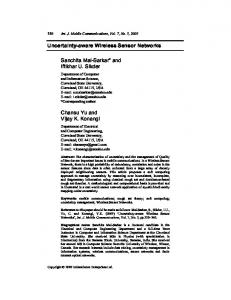
Figure 3: TMOS basic operation
and fault tolerant systems. Examples include solutions for distributed systems in general [15, 25], for mobile computing systems [22, 27], and as part of total ordering multicast protocols with support for causal order delivery of messages from multiple sources [2, 5, 10, 20]. However, causal message ordering is not sufficient in wireless sensor networks, since it is based on logical time.
4
THE TEMPORAL MESSAGE ORDERING SCHEME
This section describes the TMOS mechanism for temporal message ordering in detail. TMOS stands for Temporal Message Ordering in Sensor networks. We will explain the basic idea behind TMOS using the example from Section 1. Let us assume that a communication channel between any pair of nodes has the FIFO property, i.e., the messages will arrive at the receiver in the same order the sender sent them. Figure 3 shows the four nodes from the example in Section 1. Nodes 1-4 are arranged on a logical ring as indicated by the solid lines in the figure. In order to deliver sensor event m3 , node three sends two copies (m3 and m03 ) along this ring toward node four. m3 is sent clockwise, while m03 is sent counter-clockwise along the ring. After receiving m3 , node one makes sure that all locally generated sensor events are sent, and forwards m3 to node four. Likewise, after receiving m03 , node two makes sure that all locally generated sensor events are sent, and forwards m03 to node four. Similarly, if node one (two) wants to send a locally generated sensor event m1 (m2 ), it sends two copies of that event along the ring toward node four. Due to the FIFO property, node four will receive at least one copy of all events with a time stamp earlier than m3 .t before receiving the second copy of m3 . Consider for example message m1 generated by node one. Since m1 .t < m3 .t, node one will send a copy of m1 to node four before it forwards m3 received from node three. The FIFO property ensures that m1 arrives at node four before m3 .
Node four inserts all received sensor events into a list which is sorted by ascending time stamps. The first sensor event in the list (i.e., the one with the smallest time stamp) is removed and delivered to the application as soon as its second copy arrives. When the second copy of a sensor event arrives at node four, we can be sure that at least one copy of all earlier sensor events from all nodes have been received and inserted into the list. That is, a sensor event is only delivered to the application, if all messages with earlier time stamps generated by all nodes have already been delivered. This equals delivery in temporal order. TMOS consists of four major components: 1. Delivery groups: Clearly, the overhead of the above scheme depends on the number of nodes involved in temporal message ordering. On the other hand, often only sensor events generated by a certain sub-set of nodes have to be delivered in temporal order. Such a set of nodes is called a delivery group (DG). In order to achieve scalability and energy efficiency, it is important to identify small delivery groups. TMOS provides mechanisms for specifying delivery groups. 2. Ring setup: This component selects and maintains a logical ring for the nodes of a DG as depicted in Figure 3. 3. Sensor event delivery: This component deals with the delivery of sensor events to the receiver along the ring set up earlier. 4. Basic routing and transport: Sensor event delivery relies on underlying basic routing and transport mechanisms to forward a message to the next node on the ring. In the following section, we will discuss these components in detail.
4.1 Delivery Groups A delivery group is a set of sensor nodes, such that only sensor events originating from nodes in the same DG have to be delivered in temporal order. Sensor events generated by nodes in different DG can be delivered in any order. The messages generated by nodes in a DG are delivered to one or more receivers. However, for simplicity we will only consider a single receiver. We will call the nodes in the DG producers while the single receiver is called consumer. For reasons of scalability and energy efficiency, delivery groups should be as small as possible, since smaller DGs allow shorter rings, which result in fewer message transfers for the delivery of a sensor event. In order to form small DGs, TMOS provides mechanisms for producers to specify which sensor events they are going to generate, and for consumers to specify which sensor events they want to receive. For this purpose, sensor events are assumed to contain a name (such
0