13-0109
Temporal variations in the Earth’s gravity field from multiple SLR satellites: Toward the investigation of polar ice sheet mass balance K. Matsuo (1), T. Otsubo (2) (1) Graduate School of Sciences, Kyoto University. (2) Graduate School of Social Science, Hitotsubashi University.
[email protected] Abstract We derive temporal variations in the Earh’s low-degree graivy field up to degree and order 4 for the period 1986-2013 from the Satellite Laser Raning (SLR) data. Then we assess their quality by comparing with those from Gravity Recovery And Climate Experience (GRACE), Earth Orientation Paramters (EOPs), and geophysical fluid models. The degree 2 components of our SLR gravity solution are good quality in the entire period stuided here. The degree 3 and 4 components appear to suffer from low quality before 1993, whereas their qualities are improved afterwards. Our SLR gravity solution has enough capability to detect recent ice mass variations in polar regions (Greenland and Antarctica) at least after 1993 when Stella was added to the SLR constellation. Introduction Mass redistributions (water, ice, atmosphere, and crustal/mantle rocks) on the Earth alter the shape of gravity field and, as a consequent, cause a slight shift in the trajectory of artificial satellites orbiting the Earth. Satellite Laser Ranging (SLR) systems, developed in mid-1960, enable the accurate measurement of such satellite’s orbital change with a precision of better than ~1 cm[1]. Therefore, the SLR tracking data after appropriate data processing provide information on temporal variations in the Earth’s gravity field, and hence mass redistributions on the Earth. The SLR gravimetry deliver superior performance in observing the long wave-length (low-degree) gravity field variations of the Earth, which signify global-scale mass redistributions[2]. In particular, the zonal gravitational harmonic coefficient (Stokes’ coefficient) of degree 2: J2 (=-√5 C20), which represents physically the Earth’s dynamic oblateness, can be determined with the best precision of other geodetic measurements. As of now, many geophysical signatures associated with the Earth’s large-scale mass redistributions have been detected from the J2 observation by SLR. For example, the viscous rebounds of the solid Earth by glacial isostatic adjustment (GIA) in Laurentides and Fennoscandia are captured as the secular decreasing trend in the Earth’s J2 [3]. The changes in atmospheric mass and water storage on land by precipitation are mainly reflected in seasonal variation in J2 [4]. In addition, accelerated ice mass depletions in Greenland and Antarctica since 2002 due to global warming are detected as quadratic variation in J2[5][6].
In this study, we derive temporal variations in the Earth’s gravity field from the tracking data of multiple SLR satellites. Then we assess the quality of our SLR gravity solution. Here we focus on the low-degree gravity field variations with the spatial resolution of ~5000 km, which corresponds to the Stokes’ coefficients with degree and order up to 4, because SLR is not expected to be able to detect higher-degree gravity variations. As the final goal, we aim to utilize our SLR gravity solution for the investigation of long-term trend in polar ice sheet mass balance. HIT-U/SLR gravity solution The Hitotsubashi University (HIT-U) and National Institute of Information and Communications Technology (NICT) of Japan are developing an analysis software package named ‘c5++’ to consistently process various data acquired by space geodetic techniques[7][8]. This software impliments up-to-date geophysical models according to the International Earth Rotation Service (IERS) 2010 Conventions[9] to correct various perturbation forces acting to artificial satellites. Using this software package and incorporating the laser tracking data of six SLR satellites: LAGEOS 1 and 2, Starlette, Ajisai, Stella, and LARES, we obtain monthly time-series of the Stokes’ coefficients of degree and order up to 4 for 27 years between September 1986 and May 2013. Note that LAGEOS 2, Stella, and LARES were added after November 1992, Octover 1993, and April 2012, respectively, while LAGEOS 1, Starlette, and Ajisai are available in the entire period studied here. The coordinate for traking stations are kept fixed to the International Terrestrial Reference Frame (ITRF) 2008[10]. The satellite force model is based on the Earth Gravitational Model (EGM) 2008[11]. Here we refer to our SLR gravity solution as ‘HIT-U/SLR solution’. Strategy for assessing HIT-U/SLR solution In order to assess the quality of our HIT-U/SLR solution, we use the following three data sets; the satellite gravity data from Gravity Recovery And Climate Experience (GRACE), the Earth Orientation Parameters (EOPs) from space geodetic observations, and surface mass redistribution data from geophysical fluid models. Then we compare our HIT-U/SLR solution with these data sets and check their consistency. GRACE is a dedicated satellite mission to measure the Earth’s gravity field. Since its launch in 2002, GRACE has produced unprecedented high-quality gravity data with monthly temporal resolution and ~300 km spatial resolution (Stokes’ coefficients with degree and order complete to 60). Thus our HIT-U/SLR solution can be well validated by GRACE as for the later half of the studied period since 2002, except for J2 term which is known to be poorly determined by GRACE. The EOPs, that is length of days and polar motions, have been observed for several hundred years. Their measurement accuracy was drastically improved after the advent of space geodetic techniques, such as Very-Long-Baseline-Interferometry (VLBI), in these decades. The mass term of the polar motion excitations in the X (towards the Greenwich Meridian) and Y (towards 90E) can be readily converted to the changes in the Stokes’ coefficients of C21 and S21. They are also helpful to assess our HIT/U-SLR solution.
To date, various geophysical fluid models have been developed. Major portion of gravity variations are known to be caused by mass redistribution of geophysical fluids such as atmospheric mass, oceanic mass, and hydrological mass on land[13]. We here employ the Atmospheric and Ocean De-aliasing Level-1B (AOD1B) product and Global Land Data Assimilation System (GLDAS) model, to recover the atmospheric and nontidal ocean mass variations, and hydrological mass variations on land, respectively. We convert the sum of these mass variations to the Stokes’ coefficients for the period 1986-2010, during the era when these data are available. Note that ice mass variations in Greenland and Antarctica are not included because there are no publicly available models. In this paper, we focus on annual gravity variations. We fit the time-series of each Stokes’ coefficient with linear combination of linear, quadratic, and annual terms by the least squares method. The annual cosine and sine components thus extracted are compared with each other. Here we show the results of the Stokes’ coefficient of C20, S21, C30, and C44 terms. Comparison of annual gravity variation Figure 1a shows the time-series of C20 term from each observation. As described in Introduction, the secular trend of C20 in HIT-U/SLR (red broken curve) is mainly caused by GIA and recent ice mass depletions in polar regions. The annual variation of C20 is known to reflect mass redistributions by geophysical fluids. In fact, that from HIT-U/SLR (red curve) agrees well with geophysical fluid models (blue curve). In order to see the consistency of each annual variation more simply, we create phasor diagrams as shown in Figure 1c. The length and direction of each arrow indicates the amplitude and phase of each annual variation. With regard to the C20 term, all estimates show good agreement with each other in the entire period. The estimation errors before November 1992 when LAGEOS 2 data were added are relatively high (Figure 1b), but they appear to have little influence on the C20 measurement. Thus HIT-U/SLR solution provides high-quality C20 data for nearly 30 years. Figure 2a shows S21 time-series. In this term, we can use the result from the EOPs observation. As seen in Figure 2c, they all are excellently consistent with each other both in amplitude and phase. So the S21 data are also provided at a high quality level from our HIT-U/SLR analysis. The estimation error appears to decrease over time. This might be related to increasing numbers of SLR stations installed on ground. Figure 3a shows C30 time-series. It seems that high frequency noises are conspicuous in this degree. During 1987-1990, the amplitude of HIT-U/SLR annual variation is about three times as large as geophysical fluid models (Figure 3c). In addition, the phase shifts by ~60° from model, which equivalent to about 2 months gap. After the period when adding the data of Stella, the amplitude of HIT-U/SLR is settled to the same as model and GRACE, though the phase still shifts by ~50° from model and ~40° from GRACE. As a whole, however, the quality of C30 is not so bad at least after 1993. The disagreement between HIT-U/SLR and geophysical fluid model is considered to arise from two causes: incomleteness of geophysical fluid model and insensitivity of
SLR to C30 component. As described above, geophysical fluid model used here does not include ice mass variations in Greenland and Antarctica. This would partly result in disagreement with HIT-U/SLR and GRACE because mass variations there have a higher contribution to odd degee gravity components than even degree. It is speculated that the present SLR gravimetry is insensitive to odd degree gravity components (especially C30). One reason lies in low inclination angle of SLR satellite’s orbit. The inclination angle of Starlettte, LAGEOS 1, Ajisai, LAGEOS 2 are 50°, 110°, 50°, 110°, respectively. On the other hands, that of Stellte is 99°, which is near polar orbit. The satellite tracking data of polar orbit contribute a lot to determine odd degree gravity components because they include information on heterogeneity of mass redistributions between northern and southern hemisphere[14]. The other reason is the biased distribution of SLR stations installed on ground. Now about 50 SLR stations are in operation. Among them, 7 SLR stations are located in southern hemisphere. Such biased distribution would not collect information on mass heterogeneity between north and south sufficiently. Figure 4a shows C44 time-series. As you see, the time-series of HIT-U/SLR before 1993 suffer from significant noises. We cannot indentify even annual variation in the period. The phaser diagram of HIT-U/SLR at the epoch 1987-1990 has large uncertainty as indicated by the large error ellipoid. However, the quality of C44 has drastically improved afterwards. The phaser diagram of each observation at the epochs 1997-2000 and 2007-2000 show good agreement with each other. It is clear that contribution of Stella satellite to determination of higher degree gravity components is very large. Acctually, the estimation error of C44 significantly reduces after the addition of Stella data (Figure 4b). Because the orbital altitude of Stella satellie is relatively lower than other satellites (Satellite is ~800 km height whereas LAGEOS is ~5000 km), the traking data of Stella satellite is expected to be sensitive to high degree gravity components. Summary and discussion The quality of our HIT-U/SLR solution is evaluated by using GRACE, EOPs, and geophysical fluid models. The degree 2 components are determined at a high level of quality from HIT-U/SLR in the entire studied period of 1986-2013. The degree 3 components are also good quality, though they contain higher noise than degree 2 especially before 1993. It is speculated that the present SLR system might have difficulty in observing the degree 3 components by its nature. The degree 4 components are well-determined by SLR as for after the period when Stella data were added in 1993. Generally, it is very important to use the low altitude traking data by Stella satellie to constrain the higher degree gravity components. Next we discuss the availability of our HIT-U/SLR solution for the study of ice mass variations in Greenland and Antarctica. According to the GRACE observation during 2003-2010, the polar ice sheets experienced large-scale mass losses at the rates of ~390 Gt/yr, amounting to ~70% of the total ice loss globally in the same period[15]. Such extensive and massive mass losses are expected to be detected by SLR, even allowing for their limited spatial resolution. In fact, we can find the changes of long-term trend in some Stokes’ coeffients derived from HIT-U/SLR. As previous
studies suggested, the long-term GIA-induced increasing trend in C20 shifted to decreasing after around 2005 (Figure 1a). Similary, the increasing trend in S21 shifted to decreasing in the same period (Figure 2a). This was also observed by EOPs, suggesting the eastward movement of the Earth’s pole[16]. C41 time-series, not shown in this paper, also showed significant decreasing trend after 2005. These are considered to be caused by ice mass depletions in polar regions. Recently, Matsuo et al. (2013)[17] revealed that HIT-U/SLR solution allows to observe the mass variability of Greenland. Thus it can be said that SLR data can contribute to the study of ice mass variations in polar regions. In particular, it is noteworthy that SLR is expected to continue to provide useful low-degree gravity data as long as the operations are carried out, while the GRACE mission would come toward the end within the coming few years.
Figure 1. (a) C20 time-series by HIT-U/SLR (red), GRACE (green), geophysical fluid models (blue). Gray lines are the observation. Colored curves are best-fit models with linear + quadratic + annual variations. Linear + quadratic terms are shown in colored broken curves. The background colors represent the number of SLR satellites available; the light blue color means three (Starlette, LAGEOS1, Ajisai), the light red color, four (+ LAGEOS 2), the light yellow, five (+ Stella), and the light green, six (+LARES). (b) Time-series of estimation error of C20. (c) Phasor diagram of each time-series shown in (a) for the three periods; 1987-1990, 1997-2000, and 2007-2010. The horizontal axis represents amplitude of Sine component of annual variation. The vertical axis represents that of Cosine component of anuual variation. The circles at the tip of each allow show the fitting errors to annual variation.
Figure 2. (a) S21 time-series by HIT-U/SLR (red), GRACE (green), geophysical fluid models (blue), and EOPs (perpul). (b) Time-series of estimation error of S21. (c) Phasor diagram of each time-series shown in (a) for the three periods.
Figure 3. (a) C30 time-series by HIT-U/SLR (red), GRACE (green), geophysical fluid models (blue). (b) Time-series of estimation error of C30. (c) Phasor diagram of each time-series shown in (a) for the three periods.
Figure 4. (a) C44 time-series by HIT-U/SLR (red), GRACE (green), geophysical fluid models (blue). (b) Time-series of estimation error of C44. (c) Phasor diagram of each time-series shown in (a) for the three periods.
References [1] Degnan, J. J., Satellite laser ranging: Current status and future prospects, IEEE Trans. Geosci. Remote Sens., GE-32, 398-413, 1985. [2] Chao, B. F., The Geoid and Earth Rotation, Geophysical Interpretations of Geoid, ed. P. Vanicek and N. Christou, CRC Press, Boca Raton, 1994. [3] Yoder et al., Secular variation of Earth’s gravitational harmonic J2 coeffieicent from Lageos and non-tidal acceleration on Earth rotation, Nature, 303, 757-762, 1983. [4] Nerem et al., Temporal variations of the Earth’s gravitational field from satellite laser ranging to Lageos, Geophys. Res. Lett., 20, 595-598, 1993. [5] Nerem, R. S., and J. Wahr, Recent changes in the Earth’s graivy obleteness driven by Greenland and Antarctic ice mass loss, Geophys. Res. Lett., 38, L13501, 2011. [6] Cheng et al., Deceleration in the Earth’s oblateness, J. Geophys. Res. Solid Earth, 118, 1-8, 2013. [7] Otsubo T. And T. Gotoh, SLR-based TRF contributing to the ITRF2000 project, IVS 2002 General Meeting Proceedings, 300-303, 2002. [8] Hobiger et al., c5++ - Multi-technique analysis software for next generation geodetic instruments, IVS 2010 General Meeting Proceedings, 212-216, 2010. [9] Petit G. and B. Luzum, IERS Technical Note No. 36, IERS Conventions (2010), International Earth Rotation and Reference Systems Service, Frankfurt, Germany. [10] Altamimi et al., ITRF2008: An improved solution of the international terrestrial reference frame, J. Geod., 85, 457-473, 2012. [11] Pavlis et al., The development and evaluation of the Earth Gravitational Model 2008 (EGM2008), J. Geophys. Res., 117, B04406, 2012. [12] Cheng, M. K. and B. D. Tapley, Seasonal variations in low degree zonal harmonics of the Earth’s gravity field from satellite laser ranging observation, J. Geophys. Res., 104, 2667-2681, 1999. [13] Chen et al., Low degree spherical harmonic influences on Gravity Recovery And Climate Experiment (GRACE) water storage estimates, Geophys. Res. Lett., 32, L14405, 2005. [14] Konopliv et al., A global solution for the Mars static and seasonal gravity, Mars Orientation, Phobos and Deimos masses, and Mars ephemeris, Icarus, 182, 23-50. [15] Jacob et al., Recent contribution of glaciers and ice caps to sea level rise, Nature, 482, 514-518. [16] Chen et al., Rapid ice melting drives Earth’s pole to the east, Geophys. Res. Lett., 40, 2625-2630. [17] Matsuo et al., Accelerated ice mass depletion revealed by low-degree gravity field from satellite laser rangin: Greenland, 1991-2011, Geophys. Res. Lett., 40, 1-6.