(3). 148. 2008 International ITG Workshop on Smart Antennas (WSA 2008) ..... Ph.D. thesis, Chalmers University of Technology, Göteborg, Sweden,. ISBN/ISSN: ...
TENSOR-BASED FRAMEWORK FOR THE PREDICTION OF FREQUENCY-SELECTIVE TIME-VARIANT MIMO CHANNELS Marko Milojevi´c, Giovanni Del Galdo, and Martin Haardt Ilmenau University of Technology, Communications Research Laboratory, P.O. Box 100565, 98684 Ilmenau, Germany {marko.milojevic, martin.haardt}@tu-ilmenau.de
ABSTRACT In this contribution we propose a tensor-based framework for the prediction of time-variant frequency-selective MultipleInput Multiple-Output (MIMO) channels from noisy channel estimates. This method performs the prediction in a transformed domain obtained via the higher order singular value decomposition (HOSVD), namely on the transformed tensor elements. This is followed by the inverse transformation of the predicted transformed tensor elements onto a basis corresponding to the signal subspace. To verify our strategy, we compare the results in terms of the normalized mean square error using a known prediction method, e.g., a Wiener filter, applied to the transformed tensor elements with the identical method applied directly to the channel coefficients. The results of our investigation show that the tensor-based prediction method outperforms the direct prediction method. Although we concentrate in this contribution on the prediction in the time domain, this framework can also be used for the estimation in other domains. 1. INTRODUCTION Channel prediction has been studied in numerous contributions. It is an important tool to enhance the performance of wireless communication systems beyond 3G [1], where time variant frequency selective MIMO channels are exploited with OFDM techniques. Channel prediction combats efficiently feedback delay and is beneficial for adaptive modulation, power control, MIMO precoding, and multi-user scheduling. It is shown in [2, 3] that imperfect channel state information degrades the OFDM system performance, and that channel prediction improves the system performance. Performance of channel prediction with linear filters and quadratic Volterra filters is discussed in [4]. It is found that linear filters have a limited performance for long range prediction. On the other hand, the least squares solution for quadratic filters relies on accurate estimates of fourth order moments, which limits its use. A nonlinear channel predictor using the Multivariate Adaptive Regression Splines (MARS) is proposed in [5]. It
is able to detect the statistical dependence of time-varying channels better than linear filters, yielding a longer prediction interval. The modified Root-MUSIC and ESPRIT algorithms are used to model and predict the time-varying channels in [6] and [7], respectively. In [7] it is shown that channel prediction at different frequencies jointly performs better than channel prediction over every single frequency separately. In [8] a low complexity short range channel prediction using polynomial approximation is proposed. The MMSE channel predictor is introduced and improved in [9] and [10], respectively. The adaptive normalized least-mean square (NLMS) and recursive least squares (RLS) channel predictors for OFDM systems are introduced in [10]. The NLMS algorithm showed lower computational complexity but a worse performance than the RLS algorithm. A lower bound on the channel prediction error for MIMO channels is derived using the Cramer-Rao lower bound in [11]. Moreover, it is concluded that MIMO channels can be predicted longer in the future than Single-Input SingleOutput (SISO) channels. Channel prediction schemes based on Kalman filtering are proposed in [12, 13, 14]. In [15] the channel prediction based on polarimetric modeling is studied. The time-variant flat-fading channel prediction based on discrete prolate spheroidal sequences is studied in [16]. Reference [17] introduces subspace-based channel prediction. In contrast to the methods reviewed above, in this contribution we present a time variant frequency selective MIMO tensorbased channel prediction framework: the prediction is performed in a transformed domain, namely on the transformed tensor elements, instead of the channel prediction performed directly on the channel coefficients. Different filter prediction structures can be used, e.g., linear filters, non-linear filters, adaptive prediction filters, etc. In this paper we combine a tensor-based prediction framework with a simple linear filter, in order to compare it with the direct channel prediction. The paper is organized as follows: the tensor-based channel prediction framework is described in Section 2, simulation results for specific yet realistic scenarios are presented in Section 3, and Section 4 draws the conclusions.
147 c 2008 IEEE 978-1-4244-1757-5/08/$25.00 �
2. TENSOR BASED CHANNEL PREDICTION FRAMEWORK
denote the tensor element corresponding to the channel between the r-th receive and q-th transmit antenna at baseband frequency fi = iΔf and time tj = jΔt, where Δt and Δf are the time sampling interval and the subcarrier spacing of the system under consideration, respectively. Let H(tn ) (tn denotes the time index of the last known sample) be the sub-tensor of the tensor H, containing the elements hr,q,i,j , where r ∈ {1, 2, ..., MR }, q ∈ {1, 2, ..., MT }, i ∈ F := {− N2f + 1, − N2f + 2, . . . , N2f }, and j ∈ T := {n − NTs + 1, n − NTs + 2, . . . , n}. Here the current time and the number of sub-tensor time snapshots are denoted by tn and NTs , respectively. The values NTs and Nf should be chosen such that NTs Δt is close to the coherence time, while Nf Δf is close to the coherence bandwidth of the channel. In Fig. 1 the 4-D tensor channel representation is depicted.
The higher order singular value decomposition (HOSVD) of an N th-order tensor is defined for every complex tensor H of size (I1 × I2 × ... × IN ). According to [18], we write the tensor H as H = S×1 U1 ×2 U2 ...×N UN ,
(1)
where ×n denotes the n-mode product of a tensor by a matrix, each Un is a unitary (In × In ) matrix consisting of n-mode singular vectors, and S ∈ CI1 ×I2 ×...×IN is the core tensor. The tensor S has two significant properties: i) Orthogonality: if a �= b two sub-tensors S in =a (the nth dimension is set to the fixed value a) and S in =b are orthogonal for all possible values of n, a, and b.
f- 2
ii) Ordering: the higher-order norms of a tensor ||S in =l ||H , (n) l = 1, 2, ...In , denoted also as σl , are n-mode singular values of H with the following property:
f
f2
1
f
1
t
||S in =1 ||H ≥ ||S in =2 ||H ≥ ... ≥ ||S in =In ||H ≥ 0 The n-mode product H×n U of a tensor H ∈ CI1 ×I2 ×...×IN by a matrix U ∈ CJn ×In is an (I1 × I2 × ... × In−1 × Jn × In+1 ... × IN ) tensor whose elements are calculated as (H ×n U )i1 ...in−1 jn in+1 ...iN =
�
Hi1 i2 ...iN ujn in ,
(2)
in
where the subscripts i1 ...iN denotes the indices of the corresponding tensor dimensions (e.g., Ui1 i2 is an element of the matrix U with row index i1 and column index i2 ). The HOSVD decomposition in case of a two dimensional tensor (matrix) reduces to the SVD decomposition. For more details on the HOSVD see [18, 19, 20]. The sampled channel impulse response (CIR) of a timevariant frequency-selective MIMO channel can be represented by a four-dimensional tensor H(exact) ∈ CMR ×MT ×Nf ×NT , where MR and MT are the number of antenna elements at the receiver and at the transmitter, whereas Nf and NT are the number of snapshots sampled in the frequency and the time domain, respectively. We assume that the past noisy channel estimates are available. If we group the last NT noisy time snapshots for all antennas and frequencies, they form the estimated channel tensor H ∈ CMR ×MT ×Nf ×NT . In this paper we focus on the short term prediction in the time domain for all antenna elements and frequencies. Let hr,q,i,j 1 The scalar product of two tensors S, B ∈ CI1 ×I2 ×...×IN is symbolized by �S, B� and computed by summing the element-wise product of S and B∗ over all indices, where ∗ denotes complex conjugation. The scalar product allows us to define the higher-order norm of a tensor S as . p ||S||H = �S, S�.
148
tn
MT
for all values of n.
MR
t
Future (Predicted)
tn
MT
Past
MR
(Known)
Fig. 1. 4-D tensor channel representation. Knowing NT · Nf noisy MIMO channel estimates from (exact) the past, we predict the exact channel coefficients hr,q,i,p , where p = n + P is the index of the future time snapshot at the prediction horizon. Prediction at time instances that are not multiples of a time sampling interval Δt can be performed via an interpolation. The value of the prediction horizon P depends on system specific parameters. A realistic example is discussed in Section 3. By using the HOSVD we carry out the prediction on the transformed tensor coefficients instead of the channel coefficients. To calculate the transformed tensor, (n) (n) (n) first the matrices Un = [u1 u2 ... uIn ], n = 1, 2, ..., N , (n)
consisting of n-mode singular vectors ul , l = 1...In , which efficiently describe the tensor signal subspace, must be determined. They can be calculated as the matrix of left singular vectors of the n-th unfolding, n = 1, 2, ..., N [18]. For the tensor-based prediction we operate within the coherence time and coherence bandwidth of the channel, while the antenna array elements are fixed. Therefore, we assume that the bases Um , m �= k, where k is the prediction or estimation dimension (here time) are constant in the vicinity of the observed present channel coefficients hr,q,i,n . After obtaining the matrices Um , the transformed tensor A can be computed as H H H A = H×1 U1H ...×k−1 Uk−1 ×k+1 Uk+1 ...×N UN = H H×1 U1H ×2 U2H ...×N UN ×k Uk = S×k Uk ,
2008 International ITG Workshop on Smart Antennas (WSA 2008)
(3)
where (·)H denotes the Hermitian transpose and k is the prediction dimension. Note, that the equation (3) is generalized to an N dimensional tensor, although we deal here with the 4-D tensor. Let A(tj0 ) denote the transformed tensor from (3) calculated from the known estimated channel subtensor H(tj0 ) with the use of matrices Un , n �= k obtained from the whole tensor H, and let ar,q,i,j (tj0 ) be the corresponding transformed tensor elements. By doing this, the channel changes in the time domain are represented in tensors A(tj0 ). As an example, we use a linear prediction filter. To perform prediction at the time p = n + P with the linear filter, we calculate the transformed tensors A(tn−N0 +1 ), A(tn−N0 +2 ),..., A(tn ) to track its change in time, where N0 is the number of sub-tensors. Let us denote the prediction filter function as F (·). Now we can predict the transformed tensor elements at the future time p = n + P based on the knowledge of the transformed tensor elements from the past: a ˆr,q,i,j (tp ) = F (ar ,q,i,j (tj0 ))
(4)
for every value of r, q, i and j, where j0 ∈ {n − N0 + 1, n − ˆ denotes the prediction in the fuN0 + 2, . . . , n}, and (·) ture. For comparison, the same prediction function is applied directly on the channel coefficients: ˆ r,q,i,p = F (hr,q,i,j ) h 0
(5)
for every value of r, q and i, where j0 ∈ {n − N0 + 1, n − N0 + 2, . . . , n}. If the time window T used for the tensor calculation is comparable to the coherence time of the channel and if the channel is composed of multi-path components whose directions of arrivals and directions of departures change slowly in time, the channel will span a common signal subspace so that a reduced number rn , n = 1, 2, ...N , of basis vectors per tensor dimension n is sufficient to represent it. Here 0 < rn ≤ In . Therefore, it is possible to predict ˆ H(exact) (tp ) using a low rank approximation of A: ˆ H
(exact)
[r ]
ˆ (tp ) = A
[s]
[rk−1 ] [r ] (tp )×1 U1 1 ...×k−1 Uk−1 [rk+1 ] [r ] ×k+1 Uk+1 ...×N UN N .
(6)
Here Un n ∈ CIn ×rn , n = 1, 2, ...N , is the matrix consisting of rn n-mode singular vectors (defining the signal subspace) corresponding to the rn strongest n-mode singular valˆ [s] (tp ) ∈ Cr1 ×r2 ...×rN is the predicted truncated ues, and A transformed tensor consisting of elements corresponding to the signal subspace singular vectors. We denote this method as tensor − based channel prediction. The prediction performed directly on the estimated channel coefficients is denoted as direct channel prediction. The prediction of the transformed tensor elements rather than the channel elements themselves has the advantage of a reduced time variance and an inherent spatial noise filtering. That has been shown in [21] for its matrix valued counterpart. For the tensor antenna dimensions (the first and the second dimension) only the dominant basis vectors map the strongest multi-path components,
while the remaining basis vectors map either the diffuse multipath component or the estimation noise. Several filter structures F (·) can be used for the prediction on the future transformed tensors coefficients or for the direct ˆ r,q,i,p : linear filters [4], prediction of the channel coefficients h non-linear filters [5], adaptive prediction filters [10, 12, 13] etc. To make a fair comparison between tensor-based and direct channel prediction, we perform tensor-based prediction and direct channel prediction, as formulated in (4) and (5), using identical filter structure F (·). Thus, the prediction of a time variant frequency selective MIMO channel is partitioned into MR · MT · Nf SISO channel predictions. In this contribution we use a Wiener filter, described in the following. Let y(j) be the value of the complex variable y at time instant jΔt. We predict y at time (n + P )Δt, namely yˆ(n + P ), in the future based on the known samples of y up to the present time nΔt. Let the vector φ(n) contain a set of known N0 − P samples: φ(n) = [y(n − P ) y(n − P − 1) ... y(n − N0 + 1)]T , (7) where (·)T denotes the transpose operator. The weighting vector w(n) is then calculated as: w(n) = (φ(n)H φ(n))−1 φ(n)∗ y(n) ∈ CN0 −P ×1 ,
(8)
where (·)∗ denotes conjugation. Let the vector θ(n) contain the last N0 − P known samples of y θ(n) = [y(n) y(n − 1) ...
y(n − N0 + P + 1)]T . (9)
Finally, the predicted value of y at time (n+P )Δt is obtained as: (10) yˆ(n + P ) = θ(n)T w(n). 3. SIMULATION RESULTS In this section we test the validity of our tensor-based prediction framework. We compare a prediction method defined in equations (7)-(10) carried out on each of MR · MT ·Nf SISO channel links in the time dimension, and the same prediction method carried out on the transformed tensor elements ar,q,i,j (tj0 ) (MR · MT · Nf · NTs predictions) as defined in (4) followed by the step in equation (6) from predicted tensor, by means of the Normalized Mean Square Error (NMSE). The ˆ which is the estimate of A, is defined NMSE of the tensor A, as ˆ − A||2 ||A H �= . (11) ||A||2H The same OFDM simulation parameters as defined in [1] are used. The basic OFDM time-frequency resource unit, named chunk, lasts for 0.3372 ms and has a bandwidth of 156.2 kHz. In our analysis we use synthetic CIRs generated with the IlmProp, a geometry based channel modelling tool for wireless communications [22]. Fig. 2 depicts a bridge-to-car
2008 International ITG Workshop on Smart Antennas (WSA 2008)
149
where E is the noise term introduced by the channel estimator containing independent and identically distributed complex Gaussian random numbers with average power σe2 . Let �ten (tp ) be the predicted channel’s normalized mean square error using the tensor-based method and �dir (tp ) the predicted channel’s NMSE employing the prediction directly on the channel coefficients, both averaged over frequency and antenna dimensions, at future time snapshot tp . The term �ten (tp ) depends on the size of T and F , and on the values rn , n = 1...N , from (6). In our simulations we used values NT Δt=5.4 ms and Nf Δf =1.25 MHz, which are close to the coherence time and coherence bandwidth of the channel, respectively. Fig. 3 shows the absolute values of the tensor nmode singular values in all dimensions for the bridge-to-car
150
40
40
(2)
E[σ l ]
60
20 0 0
2 l
20 0 0
4
60
60
40
40
(4)
where ρ is the Signal to Noise Ratio (SNR) at the input of the channel estimator in dB. The noisy channel estimates H can be modeled as (13) H = H(exact) + E,
60
E[σ l ]
has been shown that a channel prediction with an NMSE of 0.1 leads to a minor degradation in the attained spectral efficiency. An upper limit of 0.15 for the allowed NMSE has been chosen in [1]. In investigations presented in [26], the channel estimation error is approximated by white Gaussian noise. The power σe2 of the normalized mean square channel estimation error is modeled as: � −ρ − 13 dB, ρ < 17 dB 2 (12) σe = −30 dB, ρ ≥ 17 dB,
(n)
Note that singular values σl have to be scaled for every dimension so that the total channel power is equal to 1. That step is not done for the values in Fig. 3.
l
Fig. 2. A bridge-to-car propagation scenario generated with the IlmProp.
E[σ(1)]
M1
l
BS
scenario, averaged over all other dimensions but the observed dimension n. In all 4 dimensions the first n-mode singular value, corresponding to the strongest singular vector in that dimension, is significantly higher than the other singular values in that mode for this specific scenario. Singular vectors corresponding to very weak singular values, can be neglected (e.g. in the 3rd dimension (frequency) the singular vectors starting from the fourth) in the equation (6). Channels with rn significantly lower than In are quite common in reality. An approach to determine the number of singular vectors rn that should be taken into account in (6) to predict the channel coefficients is to use the first rn singular vectors corresponding to the rn largest singular values in the signal subspace. Since the noise is white Gaussian (equation (12)) it is expected that the noise contributes the same value to all eigenvalues defining the eigenvalue threshold: only rn eigenvectors corresponding to the eigenvalues higher than this threshold are used in (6). Since the n-th tensor dimension has In n-mode singular val(n) ues, the eigenvalue threshold σth for the n-th tensor dimension can be estimated as: � σe2 (n) . (14) σth = In
E[σ(3)]
scenario, the propagation environment which we use here for the discussion of the simulation results. In this scenario the 4-element Uniform Linear Array (4-ULA) mobile terminal is moving with a speed of 50 km/h on the highway, while a second 4-ULA, acting as base station (BS), is mounted on the bridge crossing over the highway. The channel parameters (delay spread, Doppler spread, etc.) of the channels created with the IlmProp match very closely measured channel parameters in the corresponding scenario [23]. In [24, 25], it
20 0 0
5 l
10
2 l
4
10 l
20
20 0 0
(n)
Fig. 3. Singular values σl of the tensor corresponding to the n-th dimension of the channel. The index n corresponds to the following channel dimensions: 1 - Receive antenna domain, 2 - Transmit antenna domain, 3 - Frequency domain, 4 - Time domain In Fig. 4, we compare �ten (tp ) and �dir (tp ) for different SNR values and different prediction horizons (tp ). Additionally, we show the performance of the matrix-based subspace
2008 International ITG Workshop on Smart Antennas (WSA 2008)
prediction presented in [17]. Its NMSE averaged over frequency and antenna dimensions at the future snapshot tp is denoted as �mat (tp ). For the observed scenario �ten (tp ) is lower since the tensor based prediction includes the singular vectors corresponding to the strongest singular values (signal subspace) while neglecting most of the noise subspace. Moreover, the tensor-based subspace channel prediction performs better than the matrix-based subspace channel prediction since it is able to assess better the properties of the timevariant frequency-selective MIMO channels [27] especially for large prediction horizons and high SNR values. The tensor based prediction method outperforms the direct prediction method when the noise level is well determined. The performance difference is bigger for low SNR values, where the proposed method reduces the NMSE significantly. If there were no channel estimation errors, the best result would be obtained by the use of all singular vectors. If the noise level value is not determined appropriately, we might neglect a part of the signal subspace or include the noise and therefore increase prediction errors. In Fig. 4 the asymptotic behavior of two prediction methods can be noticed: at high SNRs and low prediction horizons the prediction error �dir (tp ) approaches �ten (tp ). The tensor-based prediction complexity is significantly higher than the direct prediction complexity, mostly due to the HOSVDs and a multiple n-mode products of a tensor with a matrices that have to be performed. The low rank approximation (6) reduces the computational complexity twofold: 1) the n-mode products have less multiplications and additions, and 2) not all but r1 · r2 ... · rk−1 · rk+1 ... · rN transformed tensor coefficients in (4) have to be predicted. Additionally, since the core tensor is approximately constant for N0 + P sub-tensors it does not have to be calculated at each time step. Similar investigations have been performed for Non Line-Of-Sight (NLOS) mobile scenarios where we have richer scattering than in the LOS environments. There the tensor-based prediction again outperforms the direct prediction, with the performance gap being lower as in the LOS case. 4. CONCLUSIONS
Fig. 4. Resulting NMSE as a comparison between the tensorbased and matrix-based subspace channel predictions and the direct channel prediction because it captures better the multidimensional nature of the channel, especially for large prediction horizons and high SNR values. 5. REFERENCES [1] “D2.4: Assessment of adaptive transmission technologies,” Tech. Rep. IST-2003-507581 (available at https://www.ist-winner.org/), WINNER, February 2005. [2] S. Ye, R. Blum, and L. Cimini, “Adaptive modulation for variable rate OFDM systems with imperfect channel information,” in Proc. Vehicular Technol. Conference, vol. 2, Birmingham, AL, 2002. [3] M. R. Souryal and R. L. Pickholtz, “Adaptive modulation with imperfect channel information in OFDM,” in Proc. IEEE ICC, 2001. [4] T. Ekman, G. Kubin, M. Sternad, and A. Ahlén, “Quadratic and linear filters for mobile radio channel prediction,” in Proc. IEEE Vehicular Technology Conference, VTC Fall 1999, Amsterdam, The Netherlands, 1999. [5] T. Ekman and G. Kubin, “Nonlinear prediction of mobile radio channels: measurements and MARS model designs,” in Proc. IEEE International Conference on Acoustics, Speech and Signal Processing, Phoenix, AR, 1999.
Hwang and J. Winters, “Sinusoidal modeling and prediction of fast In this contribution we propose a tensor-based prediction frame- [6] J. fading processes,” in Proc. IEEE GLOBECOM, 1998. work for time-variant frequency-selective MIMO channels from [7] L. Dong, G. Xu, and H. Ling, “Prediction of fast fading mobile ranoisy channel estimates. This method performs the predicdio channels in wideband communication systems,” in Proc. IEEE tion on the transformed tensor elements while predicting only GLOBECOM ’01, San Antonio, TX, 2001. the signal subspace of the channel. The proposed frame[8] Z. Shen, J. G. Andrews, and B. L. Evans, “Short range wireless channel work is compared with a direct channel prediction technique prediction using local information,” in Proc. IEEE Asilomar Conf. on Signals, Systems, and Computers, Pacific Grove, CA, USA, 2003. with respect to the normalized mean square errors of the pre[9] D. Schafhuber, G. Matz, and F. Hlawatsch, “Predictive equalization dicted channels. The tensor-based prediction framework outof time-varying channels for coded OFDM/BFDM systems,” in Proc. performs the direct prediction method. In the analyzed sceIEEE GLOBECOM 2000, San Francisco, November 2000, pp. 721– narios, the NMSE improvement is higher for lower SNR regimes 725. of the estimated channel. Moreover, the tensor-based sub[10] D. Schafhuber, G. Matz, and F. Hlawatsch, “Adaptive prediction of space prediction framework for time-variant frequency-selective time-varying channels for coded OFDM systems,” in Proc. ICASSP MIMO channels outperforms its matrix valued counterpart 2002, Orlando, FL, USA, May 2002.
2008 International ITG Workshop on Smart Antennas (WSA 2008)
151
[11] T. Svantesson and A. Swindlehurst, “A performance bound for prediction of a multipath MIMO channel,” in Proc. 37th Asilomar Conference on Signals, Systems, and Computers, Pacific Grove, CA, 2003. [12] C. Komninakis, C. Fragouli, A.H. Sayed, and R.D. Wesel, “Multi-input multi-output fading channel tracking and equalization using Kalman estimation,” in Proc. IEEE Trans. on Signal Processing, 50(5), May 2002. [13] M. Sternad and D. Aronsson, “Channel estimation and prediction for adaptive OFDMA/TDMA uplinks, based on overlapping pilots,” in Proc. IEEE International Conference on Acoustics, Speech and Signal Processing (ICASSP 2005), Philadelphia, PA, USA, 2005. [14] M. Sternad and D. Aronsson, “Channel estimation and prediction for adaptive OFDM downlinks,” in Proc. IEEE VTC 2003-Fall, Orlando, FL, 2003. [15] M. Chen, Radio Channel Prediction Based on Parametric Modeling, Ph.D. thesis, Chalmers University of Technology, Göteborg, Sweden, ISBN/ISSN: 978-91-7385-009-4, CPL 50782. [16] T. Zemen, C. F. Mecklenbräuker, and B. H. Fleury, “Time-variant channel prediction using time-concentrated and band-limited sequences,” in IEEE International Conference on Communications (ICC), Istanbul, Turkey, 2006. [17] M. Milojevi´c, G. Del Galdo, V. Stankovi´c, and M. Haardt, “Subspacebased framework for the prediction of MIMO OFDM channels,” in Proc. of 11th International OFDM-Workshop, Hamburg, Germany, 2006. [18] L. De Lathauwer and J. Vandewalle, “Dimensionality reduction in higher-order signal processing and rank-(r1 , r2 , ..., rn ) reduction in multilinear algebra,” in Linear Algebra and its Applications, Special Issue on Linear Algebra in Signal and Image Processing, vol. 391, pp. 31-55, 2004. [19] L. De Lathauwer, B. De Moor, and J. Vandewalle, “On the best rank1 and rank-(r1 , r2 , ..., rn ) approximation and applications of higherorder tensors,” in Society for Industrial and Applied Mathematics J. Matrix Anal. Appl., vol. 21, no. 4, pp. 1324-1342, 2000. [20] L. De Lathauwer, B. De Moor, and J. Vandewalle, “A multilinear singular value decomposition,” in Society for Industrial and Applied Mathematics J. Matrix Anal. Appl., vol. 21, no. 4, pp. 1253-1278, 2000. [21] G. Del Galdo, M. Haardt, and M. Milojevi´c, “A subspace-based channel model for frequency selective time variant MIMO channels,” in Proc. 15th Int. Symp. on Personal, Indoor, and Mobile Radio Communications (PIMRC), Barcelona, Spain, 2004. [22] G. Del Galdo, Geometry-based Channel Modeling for Multi-User MIMO Systems and Applications, Ph.D. thesis, Ilmenau University of Technology, Ilmenau, Germany, ISBN: 978-3-938843-27-7, available to download at http://www.delgaldo.com. [23] “WINNER 1 WP5: "Final report on link level and system level channel models" deliverable D5.4,” Tech. Rep. IST-2003-507581 (available at https://www.ist-winner.org/), WINNER, November 2005. [24] S. Falahati, A. Svensson, T. Ekman, and M. Sternad, “Adaptive modulation systems for predicted wireless channels,” IEEE Trans. on Communications, Feb. 2004. [25] S. Falahati, A. Svensson, M. Sternad, and H. Mei, “Adaptive trelliscoded modulation over predicted flat fading channels,” in Proc. IEEE VTC 2003-Fall, Orlando, FL, 2003. [26] “D2.1: Identification of radio-link technologies,” Tech. Rep. IST-2003507581 (available at https://www.ist-winner.org/), WINNER, June 2004. [27] M. Weis, G. Del Galdo, and M. Haardt, “A correlation tensor-based model for time variant frequency selective MIMO channels,” in International ITG/IEEE Workshop on Smart Antennas (WSA’07), Vienna, Austria, 2007.
152
2008 International ITG Workshop on Smart Antennas (WSA 2008)